Kinetic and hydrodynamic models of chemotactic aggregation

Abstract

We derive general kinetic and hydrodynamic models of chemotactic aggregation that describe certain features of the morphogenesis of biological colonies (like bacteria, amoebae, endothelial cells or social insects). Starting from a stochastic model defined in terms of $N$ coupled Langevin equations, we derive a nonlinear mean field Fokker-Planck equation governing the evolution of the distribution function of the system in phase space. By taking the successive moments of this kinetic equation and using a local thermodynamic equilibrium condition, we derive a set of hydrodynamic equations involving a damping term. In the limit of small frictions, we obtain a hyperbolic model describing the formation of network patterns (filaments) and in the limit of strong frictions we obtain a parabolic model which is a generalization of the standard Keller-Segel model describing the formation of clusters (clumps). Our approach connects and generalizes several models introduced in the chemotactic literature. We discuss the analogy between bacterial colonies and self-gravitating systems and between the chemotactic collapse and the gravitational collapse (Jeans instability). We also show that the basic equations of chemotaxis are similar to nonlinear mean field Fokker-Planck equations so that a notion of effective generalized thermodynamics can be developed.

Key words: Nonlinear mean field Fokker-Planck equations, generalized thermodynamics, chemotaxis, gravity, long-range interactions

1 Introduction

In many fields of physical sciences, one is confronted with the description of the evolution of a system of particles which self-consistently attract each other over large distances [1, 2]. This is the case in biology, for example, in relation with the process of chemotaxis [3]. Chemotaxis explains the spontaneous self-organization of biological cells (bacteria, amoebae, endothelial cells,…) or even insects (like ants) due to the long-range attraction of a chemical (pheromone, smell, food,…) produced by the organisms themselves. The chemotactic aggregation of biological populations is usually studied in terms of the Keller-Segel model consisting in two coupled differential equations [4]:

$${\partial\rho\over\partial t}=D_{*}\Delta\rho-\chi\nabla\cdot(\rho\nabla c),$$ (1)

$${\partial c\over\partial t}=-k(c)c+h(c)\rho+D_{c}\Delta c,$$ (2)

which describe the evolution of the concentration $\rho({\bf r},t)$ of the biological organisms and of the secreted chemical $c({\bf r},t)$. The Keller-Segel model is a parabolic model where the evolution of the concentration of the biological organisms is governed by a drift-diffusion equation (1). The diffusion models the erratic motion of the particles (like in Brownian theory) and the drift term models a systematic motion along the gradient of concentration of the secreted chemical. When $\chi>0$ the cells are attracted in regions of high concentration while for $\chi<0$ they are repelled from the regions of high concentration (in that case the chemical acts as a poison). The evolution of the secreted chemical is described by a diffusion equation (2) involving terms of source and degradation: the chemical is produced by the organisms at a rate $h(c)$ and it is degraded at a rate $k(c)$. For $\chi>0$, the Keller-Segel model is able to reproduce the chemotactic aggregation (collapse) of biological populations when the attractive drift term $\chi\rho\|\nabla c\|$ overcomes the diffusive term $D_{*}\|\nabla\rho\|$ above a critical mass $M_{c}$ [5]. This is similar to the gravitational collapse of self-gravitating Brownian particles, described by the Smoluchowski-Poisson system, below a critical temperature $T_{c}$ [6] (see [7, 8] for a detailed discussion of the analogy between the Keller-Segel model and the Smoluchowski-Poisson system). These parabolic models ultimately lead to the formation of Dirac peaks [9, 10].

Some regularizations of the Keller-Segel model have been introduced. They have the form of generalized drift-diffusion equations [11, 7]:

$${\partial\rho\over\partial t}=\nabla\cdot\left(\chi\left(\nabla p-\rho\nabla c\right)\right),$$ (3)

$${\partial c\over\partial t}=-k(c)c+h(c)\rho+D_{c}\Delta c,$$ (4)

in which the simple diffusion term $D_{*}\nabla\rho$ in Eq. (1) is replaced by a more general “pressure term” $\nabla p(\rho)$. The drift-diffusion equation (3) is similar to a generalized Smoluchowski equation [12, 13] . By adapting the barotropic equation of state $p(\rho)$, one can obtain regularized chemotactic models preventing the density from reaching infinitely large values and forming singularities [14]. In that case, the Dirac peaks (clumps) are replaced by smoother density profiles (aggregates). The dynamical evolution of the regularized model (3)-(4) generically leads to the formation of ${\cal N}(t)$ round aggregates which progressively merge until only one big aggregate remains at the end.

However, recent experiments of in vitro formation of blood vessels show that cells randomly spread on a gel matrix autonomously organize to form a connected vascular network that is interpreted as the beginning of a vasculature [15]. This phenomenon is responsible of angiogenesis, a major actor for the growth of tumors. These networks cannot be explained by the parabolic models (1)-(4) that lead to pointwise blow-up or round aggregates. However, they can be recovered by hyperbolic models that lead to the formation of networks patterns that are in good agreement with experimental results. These models take into account inertial effects and they have the form of hydrodynamic equations [15]:

$${\partial\rho\over\partial t}+\nabla\cdot(\rho{\bf u})=0,$$ (5)

$$\frac{\partial{\bf u}}{\partial t}+({\bf u}\cdot\nabla){\bf u}=-{1\over\rho}\nabla p+\nabla c,$$ (6)

$${\partial c\over\partial t}=-k(c)c+h(c)\rho+D_{c}\Delta c.$$ (7)

The inertial term models cells directional persistence and the general density dependent pressure term $-\nabla p(\rho)$ can take into account the fact that the cells do not interpenetrate. In these models, the particles concentrate on lines or filaments. These structures share some analogies with the formation of ants’ networks (due to the attraction of a pheromonal substance) and with the large-scale structures in the universe that are described by similar hydrodynamic (hyperbolic) equations: the so-called Euler-Poisson system. The similarities between the networks observed in astrophysics (see Figs 10-11 of [16]) and biology (see Figs 1-2 of [15]) are striking.

The above-mentioned parabolic and hyperbolic models are continuous models which describe the evolution of a smooth density field $\rho({\bf r},t)$ and, in the case of hyperbolic models, a smooth velocity field ${\bf u}({\bf r},t)$. In this paper, we propose a kinetic derivation of these models starting from a microscopic description of the dynamics of the biological population. We introduce stochastic equations for the motion of each individual and, implementing a mean field approximation, we obtain the corresponding Fokker-Planck equation governing the evolution of the distribution function $f({\bf r},{\bf v},t)$ of the system in phase space. The stochastic Langevin equations involve a friction force, an effective force due to the chemotactic attraction of the chemical and a random force (noise) whose strength can depend on the local distribution function itself. This dependence can take into account microscopic constraints (“hidden constraints”) that affect the dynamics of the particles at small scales. We can have (i) close packing effects (like finite size effects, excluded volume constraints, steric hindrance…) that forbid the interpenetration of the particles and prevent the system from reaching arbitrarily high densities [14] and (ii) nonextensivity effects that alter the usual random walk and lead to anomalous diffusion and non-ergodic behaviour [17, 18]. The resulting generalized stochastic equations lead to nonlinear mean field Fokker-Planck equations similar to those occurring in the context of generalized thermodynamics [19, 12, 11]. Therefore, as first noticed in [11], the chemotaxis of biological populations can be a physical system where a notion of effective generalized thermodynamics applies. By taking the successive moments of these generalized Fokker-Planck equations and using a local thermodynamic equilibrium condition, we derive a closed set of hydrodynamic equations

$${\partial\rho\over\partial t}+\nabla\cdot(\rho{\bf u})=0,$$ (8)

$$\frac{\partial{\bf u}}{\partial t}+({\bf u}\cdot\nabla){\bf u}=-{1\over\rho}\nabla p+\nabla c-\xi\rho{\bf u},$$ (9)

$${\partial c\over\partial t}=-k(c)c+h(c)\rho+D_{c}\Delta c,$$ (10)

involving a friction term $-\xi{\bf u}$ [11, 20]. For $\xi=0$, we recover the hyperbolic model (5)-(7) proposed by Gamba et al. [15] to model vasculogenesis and for $\xi\rightarrow+\infty$ we obtain the parabolic model (3)-(4) generalizing the Keller-Segel model (1)-(2). We discuss the analogy between bacterial colonies and self-gravitating systems and between the chemotactic collapse and the “gravitational collapse” (Jeans instability) [7, 8, 20]. Indeed, the kinetic and hydrodynamic models of biological populations derived in this paper are similar to those describing self-gravitating systems [11, 21]. Therefore, our approach connects various topics studied by different communities: systems with long-range interactions [1], nonlinear mean field Fokker-Planck equations and generalized thermodynamics [19], self-gravitating systems [22] and chemotaxis [4].

2 A stochastic model of chemotactic aggregation

2.1 Generalized Langevin equations

We shall introduce a model of chemotactic aggregation generalizing the Keller-Segel model (1)-(2). For biological systems, the number of constituents is not necessarily large so that it may be relevant to return to a “corpuscular” description of the system and introduce an equation of motion for each particle ($=$ cell). This type of “microscopic” approach has been previously considered by Schweitzer & Schimansky-Geier [23], Stevens [24] and Newman & Grima [25] (see also related work by the authors ). They describe the motion of individuals by a stochastic equation of the form

$${d{\bf r}_{\alpha}\over dt}=\chi\nabla_{\alpha}c+\sqrt{2D_{*}}{\bf R}_{\alpha}(t).$$ (11)

The first term in the r.h.s. is the chemotactic drift to which the particles are submitted (the coefficient $\chi$ plays the role of a mobility). The second term is a stochastic term where ${\bf R}_{\alpha}(t)$ is a white noise satisfying $\langle{\bf R}_{\alpha}(t)\rangle={\bf 0}$ and $\langle{R}_{i,\alpha}(t){R}_{j,\beta}(t^{\prime})\rangle=\delta_{ij}\delta_{\alpha,\beta}\delta(t-t^{\prime})$ (where $\alpha=1,...,N$ refer to the particles and $i=1,...,d$ to the space coordinates) and $D_{*}$ is a diffusion coefficient. The diffusion, that is observed for several biological organisms, can have different origins depending on the system under consideration [27]. In the case of small organisms moving in a fluid (matrigel), it can be due to the repeated impact of the molecules of the fluid on the particles like in ordinary Brownian motion for colloidal suspensions. In other cases, it can be due to the properties of motion of the particles themselves. For example, bacteria like Escherichia coli are equipped with flagella and are self-propelled. When rotated counterclockwise, the flagella act as a propellor and the bacterium moves along straight line (“run”). Suddenly, the flagella rotate clockwise and the bacterium stops to choose a new direction at random (“tumble”). It continues in that direction for a while until the next tumble. Therefore, the bacteria experience a random motion of their own. At the simplest level of description, this motion can be modelled by a stochastic term like in Eq. (11). These stochastic equations describe the motion of each of the $N$ particles of the colony. As indicated above, $N$ is not necessarily large so it may be of interest to treat the bacterial colony as a discrete system of particles. By contrast, the chemical that is secreted is usually described as a continuous field. Therefore, the evolution of the concentration of the chemical is governed by an equation of the form

$${\partial c\over\partial t}=-kc+D_{c}\Delta c+h\sum_{\alpha=1}^{N}\delta({\bf r}-{\bf r}_{\alpha}(t)).$$ (12)

Equations (11)-(12) have been studied in [23, 24, 25, 26]. In the mean-field approximation, they return the usual Keller-Segel model (1)-(2).

We shall generalize the model (11)-(12) in two respects. First of all, there exists biological systems for which the inertia of the particles has to be taken into account [15]. This “inertia” means that they do not respond immediately to the chemotactic drift. We propose therefore to describe the motion of each individual of the biological population by a stochastic equation of the form

$${d{\bf r}_{\alpha}\over dt}={\bf v}_{\alpha},\qquad{d{\bf v}_{\alpha}\over dt}=-\xi{\bf v}_{\alpha}+\nabla_{\alpha}c+\sqrt{2D}{\bf R}_{\alpha}(t).$$ (13)

The first term in the r.h.s. is an “effective” friction force, the second term is a force that models the chemotactic attraction due to the chemical $c$ and the last term is a random force. The friction force takes into account the fact that the velocity of the particles has the tendency to be directed along the concentration gradient $\nabla c$. This is exactly the case when $\xi\rightarrow+\infty$. In this strong friction limit, we recover the overdamped model (11) with $\chi=1/\xi$ and $D_{*}=D/\xi^{2}$. For finite values of $\xi$, the velocity will take a (relaxation) time $\tau\sim\xi^{-1}$ to get aligned with the concentration gradient. This is how an inertial effect is introduced in the model. The term $-\xi{\bf v}$ can also represent a physical friction of the organisms against a fixed matrigel. The stochastic equations (13), coupled self-consistently to the field equation (12), describe the motion of each of the $N$ particles of the colony. This completely discrete model of chemotactic aggregation, which takes into account statistical correlations between the particles, is developed in Appendix A. An exact equation for the single-cell probability distribution is derived and it is shown precisely how a mean field approximation can be implemented in the theory. In the mean-field approximation, passing to a hydrodynamical description, we obtain the model (8)-(10) with a linear (isothermal) equation of state $p=\rho T_{eff}=D\rho/\xi$.

In order to describe more general situations where the equation of state $p=p(\rho)$ is nonlinear, we shall consider a generalized class of stochastic equations where the diffusion coefficient explicitly depends on the distribution function $f({\bf r},{\bf v},t)$ of particles in phase space. These generalized stochastic equations have been introduced in [28, 11, 12, 19]. They are associated with nonlinear Fokker-Planck equations and lead to a notion of “generalized thermodynamics”. The possibility to apply this type of equations to the chemotactic problem was proposed in [11]. In order to simplify the formalism, we shall make a mean-field approximation since the start and describe the motion of each individual of the biological population by a stochastic equation of the form

$${d{\bf v}\over dt}=-\xi{\bf v}+\nabla S(c)+\sqrt{2D(f)}{\bf R}(t),$$ (14)

where the mean field force is determined by the equation

$${\partial c\over\partial t}=-k(c)c+h(c)\rho+D_{c}\Delta c,$$ (15)

where $\rho({\bf r},t)=\langle\sum_{i}\delta({\bf r}-{\bf r}_{i}(t))\rangle$ is the smooth local density of cells (the brackets denote an average over the noise). This amounts to replacing the exact density $\rho_{ex}({\bf r},t)=\sum_{i}\delta({\bf r}-{\bf r}_{i}(t))$ in Eq. (12) by the smooth density $\rho({\bf r},t)=\langle\sum_{i}\delta({\bf r}-{\bf r}_{i}(t))\rangle$. This is how the mean-field approximation is introduced in the model. For sake of generality, we have allowed the coefficients $k$ and $h$ to depend on the concentration $c$ and we have written the chemotactic force as the gradient of a function $S(c)$ of the concentration. Equations (14)-(15) will be our starting point for the chemotactic problem. This model, or the discrete model (13), is similar to the model of self-gravitating Brownian particles introduced in [6, 17, 21]. The main difference, beyond the context, is that the Poisson equation in gravity is replaced by the more general field equation (15).

2.2 Nonlinear mean field Fokker-Planck equations

We shall now derive kinetic and hydrodynamic equations associated with the stochastic model (14)-(15). Using standard methods of Brownian theory, we find that the evolution of the distribution function $f({\bf r},{\bf v},t)$ of the system is described by a generalized mean field Fokker-Planck equation of the form

$${\partial f\over\partial t}+{\bf v}\cdot{\partial f\over\partial{\bf r}}+\nabla S(c)\cdot{\partial f\over\partial{\bf v}}={\partial\over\partial{\bf v}}\cdot\biggl{[}{\partial\over\partial{\bf v}}(D(f)f)+\xi f{\bf v}\biggr{]}.$$ (16)

We have considered a relatively general class of stochastic processes (14) where the diffusion coefficient $D(f)$ can depend on the distribution function. This dependence can take into account microscopic constraints of various origin (“hidden” constraints) that affect the dynamics at small scales. These generalized stochastic processes are associated with a notion of generalized thermodynamics [19] (see also Appendix E). The case where $D(f)$ is a power law has been first considered by Borland [28] in connection with Tsallis generalized thermodynamics [29]. The case where $D(f)$ is arbitrary has been considered by Chavanis [11] in connection with nonlinear Fokker-Planck (NFP) equations associated with more general forms of entropic functionals than the Tsallis entropy. If we write the diffusion coefficient in the form $D(f)=Df[C(f)/f]^{\prime}$, where $C(f)$ is a convex function (i.e. $C^{\prime\prime}>0$), the nonlinear Fokker-Planck equation (16) can be rewritten [11]:

$${\partial f\over\partial t}+{\bf v}\cdot{\partial f\over\partial{\bf r}}+\nabla S(c)\cdot{\partial f\over\partial{\bf v}}={\partial\over\partial{\bf v}}\cdot\biggl{[}DfC^{\prime\prime}(f){\partial f\over\partial{\bf v}}+\xi f{\bf v}\biggr{]}.$$ (17)

This type of nonlinear Fokker-Planck equations can also be derived from a master equation and a Kramers-Moyal expansion by allowing the transition probabilities to depend on the occupation number in the initial and arrival states as done in Kaniadakis [30]. The case of a normal diffusion $D(f)=D$ corresponds to $C(f)=f\ln f$ leading to the usual Kramers equation (66) associated with the Boltzmann statistics. The choice $D(f)=Df^{q-1}$ corresponds to $C(f)=(f^{q}-f)/(q-1)$ leading to the polytropic Kramers equation [31, 11, 17, 18] associated with the Tsallis statistics (these examples will be worked out explicitly in Sec. 2.4).

The stationary solution of Eq. (17), which cancels both the “collision” term (r.h.s.) and the advection term (l.h.s.), is given by (see Appendix E):

$$C^{\prime}(f_{eq})=-\beta\left[\frac{v^{2}}{2}-S(c)\right]-\alpha,$$ (18)

where $\beta=1/T_{eff}$ is an effective inverse temperature satisfying a generalized Einstein relation $\beta={\xi}/{D}$ and $\alpha$ is a constant of integration. Since $C$ is convex, the above relation can be reversed. Then, we find that $f_{eq}({\bf r},{\bf v})=F(\beta\epsilon+\alpha)=f_{eq}(\epsilon)$ where $F(x)=(C^{\prime})^{-1}(-x)$. Since $f_{eq}^{\prime}(\epsilon)=-\beta/C^{\prime\prime}(f_{eq})$ and $\beta>0$, we find that $f_{eq}(\epsilon)$ is a decreasing function of the individual energy $\epsilon=v^{2}/2-S(c)$. The case of normal diffusion $D(f)=D$ leads to the Maxwell-Boltzmann distribution $f_{eq}=Ae^{-\beta\epsilon}$. The case of anomalous diffusion $D(f)=Df^{q-1}$ leads to the Tsallis distribution $f_{eq}=\left[\lambda-\beta(q-1)\epsilon/q\right]^{1/(q-1)}$ [11].

2.3 Damped hydrodynamic equations

We shall now derive the moments equations issued from the generalized Fokker-Planck equation (17). Defining the density and the local velocity by

$$\rho=\int f\,d{\bf v},\qquad\rho{\bf u}=\int f{\bf v}\,d{\bf v},$$ (19)

and integrating Eq. (17) on velocity, we get the continuity equation

$${\partial\rho\over\partial t}+\nabla\cdot(\rho{\bf u})=0.$$ (20)

Next, multiplying Eq. (17) by ${\bf v}$ and integrating on velocity, we obtain

$${\partial\over\partial t}(\rho u_{i})+{\partial\over\partial x_{j}}(\rho u_{i}u_{j})=-{\partial P_{ij}\over\partial x_{j}}+\rho S^{\prime}(c){\partial c\over\partial x_{i}}-\xi\rho u_{i},$$ (21)

where we have defined the “pressure” tensor

$$P_{ij}=\int fw_{i}w_{j}\,d{\bf v},$$ (22)

where ${\bf w}={\bf v}-{\bf u}$ is the relative velocity. Using the continuity equation, Eq. (21) can be rewritten

$$\rho\biggl{(}{\partial u_{i}\over\partial t}+u_{j}{\partial u_{i}\over\partial x_{j}}\biggr{)}=-{\partial P_{ij}\over\partial x_{j}}+\rho S^{\prime}(c){\partial c\over\partial x_{i}}-\xi\rho u_{i}.$$ (23)

By taking the successive moments of the velocity, we can obtain a hierarchy of hydrodynamic equations. Each equation of the hierarchy involves the moment of next order. If we are sufficiently close to equilibrium, it makes sense to close the hierarchy of equations by using a condition of local thermodynamic equilibrium (L.T.E.). We shall thus evaluate the pressure tensor Eq. (22) with the distribution function $f_{L.T.E}({\bf r},{\bf v},t)$ defined by the relation (see Appendix E.1):

$$C^{\prime}(f_{L.T.E.})=-\beta\biggl{[}{w^{2}\over 2}+\lambda({\bf r},t)\biggr{]}.$$ (24)

The function $\lambda({\bf r},t)$ is implicitly related to the density by writing

$$\rho({\bf r},t)=\int f_{L.T.E.}\,d{\bf v}=\rho[\lambda({\bf r},t)].$$ (25)

Using the condition Eq. (24) of local thermodynamic equilibrium, the pressure tensor Eq. (22) can be written $P_{ij}=p\delta_{ij}$ with

$$p({\bf r},t)={1\over d}\int f_{L.T.E.}w^{2}\,d{\bf w}=p[\lambda({\bf r},t)].$$ (26)

The pressure is a function $p=p(\rho)$ of the density which is entirely specified by the function $C(f)$, by eliminating $\lambda$ from the relations Eq. (25) and Eq. (26). This defines a barotropic gas. For example, the case of normal diffusion $D(f)=D$ leads to a Maxwellian distribution $f_{L.T.E.}=(\beta/2\pi)^{d/2}\rho({\bf r},t){\rm exp}(-\beta w^{2}/2)$ and a linear equation of state $p=\rho T_{eff}$ as for an isothermal gas. The case of anomalous diffusion $D(f)=Df^{q-1}$ leads to a Tsallis distribution $f_{L.T.E.}=\left[\mu({\bf r},t)-\beta((q-1)/q)w^{2}/2\right]^{1/(q-1)}$ and a power law equation of state $p=K\rho^{\gamma}$ (with $\gamma=1+1/n$ and $n=d/2+1/(q-1)$) as for a polytropic gas [17]. Substituting the result $P_{ij}=p(\rho)\delta_{ij}$ in Eq. (23) and collecting the other constitutive equations, we obtain a hydrodynamic model of the form:

$${\partial\rho\over\partial t}+\nabla\cdot(\rho{\bf u})=0,$$ (27)

$${\partial{\bf u}\over\partial t}+({\bf u}\cdot\nabla){\bf u}=-{1\over\rho}\nabla p+\nabla S(c)-\xi{\bf u},$$ (28)

$${\partial c\over\partial t}=-k(c)c+h(c)\rho+D_{c}\Delta c.$$ (29)

The damped barotropic Euler equations (27)-(29) are interesting as they connect hyperbolic models to parabolic models [11]. For $\xi=0$, we recover the hydrodynamic model (5)-(7) introduced by Gamba et al. [15] . Alternatively, for $\xi\rightarrow+\infty$, we can formally neglect the inertial term in Eq. (28) so that the velocity field is given by

$${\bf u}=-{1\over\xi\rho}(\nabla p-\rho S^{\prime}(c)\nabla c)+O(\xi^{-2}).$$ (30)

Substituting this drift term in the continuity equation (27), we obtain the drift-diffusion equation

$${\partial\rho\over\partial t}=\nabla\cdot\biggl{[}\frac{1}{\xi}\left(\nabla p-\rho S^{\prime}(c)\nabla c\right)\biggr{]},$$ (31)

which is a generalization of the Keller-Segel model. The usual Keller-Segel model is recovered for a normal diffusion $D(f)=D$ leading to $p=\rho T_{eff}=D\rho/\xi$. We make the link with Eq. (1) by setting $D_{*}=D/\xi^{2}$, $\chi=1/\xi$ and $S(c)=c$. The case of a polytropic equation of state $p=K\rho^{\gamma}$ associated to the Tsallis statistics has been studied in [17, 18].

It should be stressed that the damped Euler equations (27)-(29) remain heuristic because their derivation is based on the Local Thermodynamic Equilibrium (L.T.E.) condition (24) which is not rigorously justified. However, using a Chapman-Enskog expansion, it is shown in [33] that the generalized Smoluchowski equation (31) is exact in the limit $\xi\rightarrow+\infty$ (or, equivalently, for times $t\gg\xi^{-1}$). The generalized Smoluchowski equation can also be obtained from the moments equations of the generalized Kramers equation by closing the hierarchy in the limit $\xi\rightarrow+\infty$ (see [13] and Appendix B).

2.4 A generalized Keller-Segel model

In this section, we discuss an explicit example to illustrate our general formalism. We consider a stochastic process of the form

$${d{\bf v}\over dt}=-\xi{\bf v}+\nabla S(c)+\sqrt{2D}f^{(q-1)/2}{\bf R}(t),$$ (32)

where the mean field force is determined by Eq. (15). Comparing with Eq. (14), we find that the diffusion coefficient is given by $D(f)=Df^{q-1}$. As indicated previously, this leads to a situation of anomalous diffusion related to the Tsallis statistics [28]. For $q=1$, we recover the standard Brownian model with a constant diffusion coefficient, corresponding to a pure random walk (see Appendix A). In that case, the sizes of the random kicks are uniform and do not depend on where the particle happens to be. For $q\neq 1$, the size of the random kicks changes, depending on the phase-space distribution of the particles around the “test” particle. A particle which is in a state $({\bf r},{\bf v})$ that is highly populated [large $f({\bf r},{\bf v},t)$] will tend to have larger kicks if $q>1$ and smaller kicks if $q<1$. Since the microscopics depends on the actual density in phase space, this creates a bias in the ergodic behavior of the system. The nonlinear Fokker-Planck equation associated with the stochastic process (32) is the polytropic Kramers equation

$${\partial f\over\partial t}+{\bf v}\cdot{\partial f\over\partial{\bf r}}+\nabla S(c)\cdot{\partial f\over\partial{\bf v}}={\partial\over\partial{\bf v}}\cdot\biggl{(}D{\partial f^{q}\over\partial{\bf v}}+\xi f{\bf v}\biggr{)}.$$ (33)

For $q=1$, we recover the classical Kramers equation (66) which can be deduced from the $N$-body stochastic process (13) by using a mean field approximation (see Appendix A). For $q\neq 1$, the NFP equation (33) can be deduced from the mean field stochastic process (32). The associated Lyapunov functional (100) is explicitly given by

$$F[f]=\int f\frac{v^{2}}{2}d{\bf r}d{\bf v}+\frac{1}{2h}\int\left[D_{c}(\nabla c)^{2}+kc^{2}\right]d{\bf r}-\int\rho cd{\bf r}+\frac{T_{eff}}{q-1}\int(f^{q}-f)d{\bf r}d{\bf v},$$ (34)

where $T_{eff}=1/\beta=D/\xi$. It can be viewed as an effective generalized free energy $F=E-T_{eff}S$ associated with the Tsallis entropy $S_{q}=-(1/(q-1))\int(f^{q}-f)d{\bf r}d{\bf v}$. It satisfies $\dot{F}\leq 0$ which is the version of the $H$-theorem in the canonical ensemble where the temperature $T_{eff}$ is fixed instead of the energy. The steady state of the NFP equation (33) is the polytropic (Tsallis) distribution

$$f_{eq}=\left[\mu-\frac{\beta(q-1)}{q}\epsilon\right]^{1/(q-1)},$$ (35)

where $\epsilon=v^{2}/2-S(c)$ is the energy per particle. This distribution extremizes the free energy (34) at fixed mass. Furthermore, it is linearly dynamically stable with respect to the NFP equation (33) if, and only if, it is a minimum of $F$ at fixed $M$ [11]. The index $n$ of the polytrope (defined by Eq. (41) below) is related to the parameter $q$ by the relation

$$n=\frac{d}{2}+\frac{1}{q-1}.$$ (36)

The isothermal (Boltzmann) distribution function $f_{eq}=Ae^{-\beta\epsilon}$, corresponding to normal diffusion, is recovered in the limit $q\rightarrow 1$, i.e. $n\rightarrow+\infty$. In the following, we shall consider $q>0$ so that $C$ is convex. Since $\beta>0$, this implies that $f(\epsilon)$ is decreasing (see Sec. 2.2). There are two cases to consider. For $q>1$, i.e. $n>d/2$, the distribution (35) can be written

$$f=A(\epsilon_{m}-\epsilon)^{1/(q-1)}\quad({\rm case}\ 1)$$ (37)

where $A=[\beta(q-1)/q]^{1/(q-1)}$ and $\epsilon_{m}=q\mu/[\beta(q-1)]$. It has a compact support since $f$ is defined only for $\epsilon\leq\epsilon_{m}$. For $\epsilon\geq\epsilon_{m}$, we set $f=0$ (for $q=+\infty$, i.e. $n=d/2$, $f$ is the Heaviside function). For $q<1$ the distribution can be written

$$f=A(\epsilon_{0}+\epsilon)^{-1/(1-q)}\quad({\rm case}\ 2)$$ (38)

where $A=[\beta(1-q)/q]^{-1/(1-q)}$ and $\epsilon_{0}=q\mu/[\beta(1-q)]$. It is defined for all energies. For large velocities, it behaves like $f\sim v^{2n-d}$. Therefore, the density and the pressure are finite only for $n<-1$, i.e. $d/(d+2)<q<1$. Therefore the range of allowed parameters are

$$q>1,\qquad n>\frac{d}{2}\quad({\rm case}\ 1)$$ (39)

$$\frac{d}{d+2}<q<1,\qquad n<-1\quad({\rm case}\ 2)$$ (40)

From Eq. (35), or the alternative forms (37) and (38), we can compute the density $\rho=\int fd{\bf v}=\rho[c({\bf r})]$ and the pressure $p=(1/d)\int fv^{2}d{\bf v}=p[c({\bf r})]$ at equilibrium (see Sec. 3.6 of [34] for details). Then, eliminating the concentration $c({\bf r})$ between these expressions, we obtain the polytropic equation of state

$$p=K\rho^{\gamma},\qquad\gamma=1+{1\over n}.$$ (41)

For $n>d/2$ (case 1), the polytropic constant is

$$K=\frac{1}{n+1}\left[AS_{d}2^{\frac{d}{2}-1}\frac{\Gamma\left(d/2\right)\Gamma\left(1-d/2+n\right)}{\Gamma(1+n)}\right]^{-1/n},$$ (42)

and for $n<-1$ (case 2), we have

$$K=-\frac{1}{n+1}\left[AS_{d}2^{\frac{d}{2}-1}\frac{\Gamma\left(d/2\right)\Gamma\left(-n\right)}{\Gamma(d/2-n)}\right]^{-1/n},$$ (43)

where $\Gamma(x)$ is the Gamma function. For $q=1$, the polytropic equation of state (41) reduces to the “isothermal” (linear) equation of state $p=\rho T_{eff}$. These equations of state have been obtained from the distribution (35) valid at equilibrium. However, the same equations of state are obtained from the L.T.E condition (24), using Eqs. (25) and (26) and $C(f)=(f^{q}-f)/(q-1)$, or from the distribution function (76) valid in the strong friction limit $\xi\rightarrow+\infty$, using Eqs. (77) and (78). Then, the damped hydrodynamic equations corresponding to the model (32) are Eqs. (27)-(29) with the equation of state (41). On the other hand, in the strong friction limit, the drift-diffusion equation (31) reduces to the polytropic Smoluchowski equation

$${\partial\rho\over\partial t}=\nabla\cdot\biggl{[}\frac{1}{\xi}\left(K\nabla\rho^{\gamma}-\rho S^{\prime}(c)\nabla c\right)\biggr{]}.$$ (44)

The associated Lyapunov functional (127) is explicitly given by

$$F[\rho]={K\over\gamma-1}\int(\rho^{\gamma}-\rho)\ d{\bf r}+\frac{1}{2h}\int\left[D_{c}(\nabla c)^{2}+kc^{2}\right]d{\bf r}-\int\rho c\,d{\bf r}.$$ (45)

It can be viewed as an effective generalized free energy $F=E-KS$ associated with the Tsallis entropy $S_{\gamma}=-(1/(\gamma-1))\int(\rho^{\gamma}-\rho)d{\bf r}$ where $K$ plays the role of an effective temperature and $\gamma$ the role of the Tsallis $q$-parameter. It satisfies $\dot{F}\leq 0$ which is the version of the $H$-theorem in the canonical ensemble where the “polytropic temperature” $K$ is fixed instead of the energy. The steady state of the generalized Smoluchowski equation (44) is the polytropic (Tsallis) distribution in physical space

$$\rho_{eq}=\biggl{[}\lambda+{\gamma-1\over K\gamma}S(c)\biggr{]}^{1\over\gamma-1}.$$ (46)

This distribution extremizes the free energy (45) at fixed mass. Furthermore, it is linearly dynamically stable with respect to the generalized Smoluchowski equation (44) if and only if it is a minimum of $F$ at fixed $M$. Of course, Eq. (46) can be deduced from Eq. (35). Equation (44) can be interpreted as a NFP equation of the form considered in [11] with $C(\rho)=(\rho^{\gamma}-\rho)/(\gamma-1)$. It can be obtained directly from the generalized stochastic process (see Appendix E.4)

$$\frac{d{\bf r}}{dt}=\frac{1}{\xi}\rho\nabla S(c)+\sqrt{\frac{2K}{\xi}}\rho^{(\gamma-1)/2}{\bf R}(t).$$ (47)

This stochastic process generalizes Eq. (11) and provides another justification of the polytropic Smoluchowski equation (44). The interpretation of the noise in Eq. (47), depending on the density $\rho({\bf r},t)$, is similar to that given after Eq. (32) although the process takes place in physical space instead of phase space.

Finally, we note the remarkable feature that a polytropic distribution $f_{eq}(\epsilon)$ [see Eq. (35)] with index $q$ in phase space yields a polytropic distribution $\rho_{eq}(c)$ [see Eq. (46)] with index $\gamma$ in physical space (using Eqs. (36) and (41), the indices are related to each other by $\gamma=1+2(q-1)/[2+d(q-1)]$). In this sense, polytropic (Tsallis) distributions are “stable” laws. Apparently, these are the only ones enjoying the property that $f_{eq}(\epsilon)$ and $\rho_{eq}(c)$ have the same form. By comparing Eqs. (35) and (46) or Eqs. (34) and (45), we note that $K$ plays the same role in physical space as the temperature $T_{eff}=1/\beta$ in phase space. It is sometimes called a “polytropic temperature”. We also note that for $q>1$, we have $\gamma>1$ so that the model is hyper-diffusive in phase space and physical space. For $q<1$, we have $\gamma<1$ so that the model is sub-diffusive in phase space and physical space. For $q=1$, we have $\gamma=1$ so that Eq. (44) reduces to the ordinary Smoluchowski equation. This yields the standard Keller-Segel model [4]. For $q\neq 1$, or $\gamma\neq 1$, we obtain a generalized Keller-Segel model that can take into account non-ideal effects giving rise to anomalous diffusion. This model has been studied in [17, 18, 35].

2.5 Numerical simulations

In this section, we restrict ourselves to normal diffusion and we present numerical simulations of the $N$-body system (13)-(12) in a simplified setting. In the equation (12) for the evolution of the secreted chemical, we set $h=\lambda D_{c}$ and consider a limit of large diffusivity $D_{c}\rightarrow+\infty$ with $\lambda\sim 1$. In that limit, the temporal derivative $\partial c/\partial t$ and the degradation term $-kc$ can be neglected (see Appendix C). The model (13)-(12) becomes

$${d{\bf v}_{\alpha}\over dt}=-\xi{\bf v}_{\alpha}+\nabla_{\alpha}c+\sqrt{2D}{\bf R}_{\alpha}(t),$$ (48)

$$\Delta c=-\lambda(\rho_{ex}-\overline{\rho}),$$ (49)

where $\rho_{ex}({\bf r},t)=\sum_{\alpha=1}^{N}\delta({\bf r}-{\bf r}_{\alpha}(t))$ is the exact density and $\overline{\rho}=N/V$ is the average density over the entire domain. When $D=\xi=0$, we obtain

$${d{\bf v}_{\alpha}\over dt}=\nabla_{\alpha}c,$$ (50)

$$\Delta c=-\lambda(\rho_{ex}-\overline{\rho}).$$ (51)

These equations are similar to the Newton equations for a self-gravitating system where $-c$ plays the role of the gravitational potential $\Phi$ and $\lambda$ the role of the gravitational constant $S_{d}G$ ($S_{d}$ is the surface of a unit sphere in $d$-dimensions). In cosmology, when we take into account the expansion of the universe and work in a comoving frame, the usual Poisson equation $\Delta\Phi=4\pi G\rho$ is replaced by an equation of the form $\Delta\phi=4\pi Ga(t)^{2}[\rho({\bf x},t)-\rho_{b}(t)]$ where the density $\rho({\bf x},t)$ is replaced by the deviation $\rho({\bf x},t)-{\rho}_{b}(t)$ to the mean density [36]. Furthermore, the equations of motion read $(d/dt)(ma^{2}\dot{\bf x})=-m\nabla\phi$. If we consider timescales over which the variation of the scale factor $a(t)$ can be neglected, the equations of motion become isomorphic to Eqs. (50)-(51). Therefore, there exists interesting analogies between the process of chemotaxis in biology and the dynamics of self-gravitating systems.

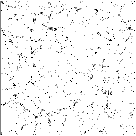
Figure 1: $N$-body simulation of the inertial model (50)-(51) for $N=32768$ particles in a periodic box. The dynamical equations are isomorphic to the Newton equations for a self-gravitating system in cosmology. They show the formation of a network pattern with a filamentary structure. In biology, this corresponds to the beginning of a vasculature.

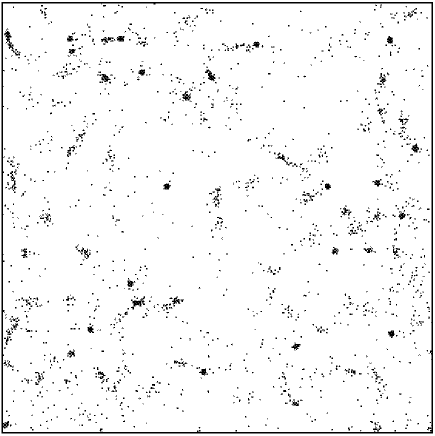
Figure 2: $N$-body simulation of the overdamped model (52)-(53) for $N=32768$ particles in a periodic box. The dynamical equations are isomorphic to the Langevin equations for a self-gravitating Brownian gas in an overdamped limit. They lead to point-wise blow-up forming ultimately Dirac peaks. In biology, this corresponds to a chemotactic collapse.

However, in biology, we are rather in a limit where inertial effects are negligible or weak so that the (effective) friction coefficient $\xi$ is relatively large. Therefore, the process of chemotaxis in biology is more directly analogous to the dynamics of self-gravitating Brownian particles studied in [6]. If we consider the strong friction limit $\xi\rightarrow+\infty$, we obtain

$${\bf v}_{\alpha}=\frac{1}{\xi}\nabla_{\alpha}c+\sqrt{2D_{*}}{\bf R}_{\alpha}(t),$$ (52)

$$\Delta c=-\lambda(\rho_{ex}-\overline{\rho}).$$ (53)

These equations are similar to those describing a self-gravitating Brownian gas in an overdamped limit [21].

The inertial model (50)-(51) leads to fluid models of a form related to Eqs. (5)-(7) that are hyperbolic. Alternatively, the overdamped model (52)-(53) leads to drift-diffusion equations of the form (1)-(2) that are parabolic. As discussed in the Introduction, parabolic models are known to lead to pointwise blow-up while hyperbolic models generate network patterns [15, 37]. We have performed direct numerical simulations of the $N$-body systems (50)-(51) and (52)-(53) in a periodic domain starting from a statistically homogeneous distribution of particles. In order to simulate a large number of particles, we have considered the dimension $d=2$ which is relevant for biological populations. The results of the simulations are reported in Figs. 1 and 2. The uniform distribution of particles is unstable (this is similar to the Jeans instability in astrophysics) and the particles start to collapse and form aggregates. Note that the concentration can be quite large although this is not always obvious on the figures since the particles have fallen on each other. Density contrasts are easier to see in continuous (fluid) models that automatically involve a coarse-graining [15, 37]. However, our $N$-body simulations also show the formation of lines and filaments in the case of models with inertia (Fig. 1) and the absence (or reduction) of such lines and the generation of pointwise blow-up in the case of overdamped systems (Fig. 2).

3 Conclusion

In this paper, we have introduced general kinetic and hydrodynamic models of chemotactic aggregation. These models can be relevant to describe the organization of social insects (swarms) like ants or the morphogenesis of biological populations like bacteria, amoebae, endothelial cells etc. Starting from a microscopic model defined in terms of $N$ coupled stochastic equations (13)-(12) or (14)-(15), we have derived a generalized mean field Fokker-Planck equation (17) governing the evolution of the distribution function of the system in phase space. By taking the successive moments of this kinetic equation and closing the hierarchy by a local thermodynamic equilibrium condition, we have derived a set of hydrodynamic equations (27)-(29) involving a damping term. An interest of this approach is to connect and generalize different models previously introduced in the literature. In particular, the Keller-Segel model (1)-(2) and the generalized Keller-Segel model (3)-(4) are obtained in a limit of strong friction $\xi\rightarrow+\infty$ and the hydrodynamic model introduced by Gamba et al. (5)-(7) corresponds formally to a limit of low friction $\xi\rightarrow 0$ (in fact, the justification of this model must be given separately as in Appendix D). We have illustrated numerically the difference between models with inertia (hyperbolic) leading to network patterns and models without inertia (parabolic) leading to pointwise blow-up. We have discussed the analogy between the chemotactic collapse in biology and the gravitational collapse (Jeans instability) in astrophysics (see also [20]).

In our kinetic model of Sec. 2.2, the dynamical evolution of bacterial populations is described by generalized stochastic processes (14) and nonlinear mean field Fokker-Planck equations (17) similar to those arising in the context of generalized thermodynamics [11, 12, 19]. As a result, the hydrodynamic equation (28) involves a nonlinear pressure term $p(\rho)$. If we consider stochastic processes with normal diffusion (13), we obtain ordinary Fokker-Planck equations (66) leading to a linear equation of state $p(\rho)=\rho T_{eff}$ (isothermal) with $T_{eff}=D/\xi$. In the strong friction limit, this yields the Keller-Segel model (1) which is known to form singularities (Dirac peaks). In order to obtain the regularized model (3), we need to modify the stochastic equations. This has been done here by letting the diffusion coefficient depend on the local distribution of particles in phase space (see Eq. (14)). This is a phenomelogical attempt to take into account complicated microscopic constraints (like excluded volume constraints, finite size effects, short-range interactions,…) that affect the dynamics of the particles at small scales. At the level of the hydrodynamic equations, these constraints are modeled by an effective pressure term $p=p(\rho)$ which replaces the usual term $p=\rho T_{eff}$. An example of regularized Keller-Segel model where the Dirac peaks are replaced by smooth density profiles (aggregates) has been studied in [14]. In that case, the effective equation of state is $p(\rho)=-\sigma_{0}T_{eff}\ln(1-\rho/\sigma_{0})$. For dilute systems where the motion of an individual cell is not impeded by the other cells, we have $\rho\ll\sigma_{0}$ and we recover the “isothermal” equation of state $p=\rho T_{eff}$. However, modifications arise when the cells are compressed. Indeed, the equation of state departs from the isothermal one when the density approaches the maximum allowable density $\sigma_{0}$. In that case, instead of Dirac peaks, we form flat cores with density $\rho\sim\sigma_{0}$. The nonlinear pressure term $p(\rho)$ can also model a process of anomalous diffusion. This is the case in particular for the stochastic model (32) leading to a polytropic equation of state $p=K\rho^{\gamma}$. This model can take into account effects of non-ergodicity and nonextensivity. This leads to the Tsallis statistics that arises when the dynamics has a fractal or multi-fractal phase space structure [28]. The corresponding generalized Keller-Segel model (44) has been studied in detail in [17, 18, 35].

The next step is a detailed study of the models presented in this paper. This study is of interest not only in mathematical biology but also, at a more general level, in statistical mechanics. What we are studying essentially is the Dynamics and Thermodynamics of Brownian Particles with Long-Range Interactions [26]. We have furthermore introduced a general class of stochastic equations with a random force depending on the distribution function, forcing the nonlinearity in the Fokker-Planck equation. This is associated with a notion of generalized thermodynamics. Therefore, our model involves both long-range forces [1] and generalized thermodynamics (related to nonlinear Fokker-Planck equations) [19], which are two domains actively studied at the moment in statistical mechanics. Our approach shows that these topics can have applications in biology. In the overdamped limit, the dynamical equations have the form of drift-diffusion equations corresponding to the Keller-Segel model or generalizations of this model. These equations have been extensively studied in the mathematical (see the review of Horstmann [5]) and physical (see Chavanis & Sire [21] and references therein) literature. The more complicated study of kinetic equations (17)-(15) or hydrodynamic equations (27)-(29) should be considered in future works. The connection with generalized forms of Cahn-Hilliard equations when the potential of interaction is short-ranged (as noticed in [12, 33]) should also be developed (see Appendix F).

Appendix A Many-body theory of chemotactic aggregation

In this Appendix, we first develop an exact many-body theory of Brownian particles in interaction. Then, we show how a mean field approximation can be implemented in the problem. For simplicity, we assume that each particle has a normal Brownian motion, i.e. the diffusion coefficient $D$ is constant. Our approach follows the steps of Newman & Grima [25]. However, we take into account the inertia of the particles while Newman & Grima consider an overdamped limit.

Basically, the dynamical evolution of $N$ Brownian particles in interaction is described by stochastic Langevin equations of the form (13). In the biological context, the field $c$ represents the concentration of the chemical produced by the cells and it satisfies an equation of the form (12). We define the single-cell probability distribution in phase space by

$$P_{\alpha}({\bf r},{\bf v},t)=\langle\delta({\bf r}-{\bf r}_{\alpha}(t))\delta({\bf v}-{\bf v}_{\alpha}(t))\rangle,$$ (54)

where the brackets denote an average over the noise. Similarly the two-cell probability distribution in phase space is

$$P_{\alpha,\beta}({\bf r},{\bf v},t;{\bf r}^{\prime},{\bf v}^{\prime},t^{\prime})=\langle\delta({\bf r}-{\bf r}_{\alpha}(t))\delta({\bf v}-{\bf v}_{\alpha}(t))\delta({\bf r}^{\prime}-{\bf r}_{\beta}(t^{\prime}))\delta({\bf v}^{\prime}-{\bf v}_{\beta}(t^{\prime}))\rangle.$$ (55)

Integrating Eq. (12), the concentration field can be expressed in terms of the cell paths as

$$c({\bf r},t)=h\int d{\bf r}^{\prime}\int_{0}^{t}dt^{\prime}G({\bf r}-{\bf r}^{\prime},t-t^{\prime})\sum_{\alpha}\delta({\bf r}^{\prime}-{\bf r}_{\alpha}(t^{\prime})),$$ (56)

where the Green function for the chemical diffusion equation is

$$G({\bf r},t)=(4\pi D_{c}t)^{-d/2}{\rm exp}\left[-{r^{2}\over 4D_{c}t}-kt\right].$$ (57)

Taking the time derivative of $P_{\alpha}$, we get

$${\partial P_{\alpha}\over\partial t}=-{\partial\over\partial{\bf r}}\cdot\langle{\dot{\bf r}}_{\alpha}(t)\delta({\bf r}-{\bf r}_{\alpha}(t))\delta({\bf v}-{\bf v}_{\alpha}(t))\rangle-{\partial\over\partial{\bf v}}\cdot\langle{\dot{\bf v}}_{\alpha}(t)\delta({\bf r}-{\bf r}_{\alpha}(t))\delta({\bf v}-{\bf v}_{\alpha}(t))\rangle.$$ (58)

Inserting the equations of motion (13) in Eq. (58), we obtain

$${\partial P_{\alpha}\over\partial t}=-{\partial\over\partial{\bf r}}\cdot\langle{{\bf v}}_{\alpha}(t)\ \delta({\bf r}-{\bf r}_{\alpha}(t))\delta({\bf v}-{\bf v}_{\alpha}(t))\rangle+{\partial\over\partial{\bf v}}\cdot\langle\xi{{\bf v}}_{\alpha}(t)\ \delta({\bf r}-{\bf r}_{\alpha}(t))\delta({\bf v}-{\bf v}_{\alpha}(t))\rangle$$

$$-{\partial\over\partial{\bf v}}\cdot\langle\nabla_{\alpha}c\ \delta({\bf r}-{\bf r}_{\alpha}(t))\delta({\bf v}-{\bf v}_{\alpha}(t))\rangle-{\partial\over\partial{\bf v}}\cdot\langle\sqrt{2D}{\bf R}_{\alpha}(t)\ \delta({\bf r}-{\bf r}_{\alpha}(t))\delta({\bf v}-{\bf v}_{\alpha}(t))\rangle.$$ (59)

The first two terms are straightforward to evaluate. The fourth term is the standard term that appears in deriving the Fokker-Planck equation for a pure random walk; it leads to a term proportional to the Laplacian of $P_{\alpha}$ in velocity space. The third term can be evaluated by inserting the formal solution (56) in Eq. (A). This leads to the exact equation

$${\partial P_{\alpha}\over\partial t}+{\bf v}\cdot{\partial P_{\alpha}\over\partial{\bf r}}+h{\partial\over\partial{\bf v}}\cdot\int d{\bf r}^{\prime}\int_{0}^{t}dt^{\prime}\nabla G({\bf r}-{\bf r}^{\prime},t-t^{\prime})\sum_{\beta}P_{\alpha,\beta}({\bf r},{\bf v},t;{\bf r}^{\prime},t^{\prime})$$

$$={\partial\over\partial{\bf v}}\cdot\left[D{\partial P_{\alpha}\over\partial{\bf v}}+\xi P_{\alpha}{\bf v}\right],\qquad\qquad$$ (60)

where the statistical correlations are encapsulated in the two-cell distribution

$$P_{\alpha,\beta}({\bf r},{\bf v},t;{\bf r}^{\prime},t^{\prime})=\langle\delta({\bf r}-{\bf r}_{\alpha}(t))\delta({\bf v}-{\bf v}_{\alpha}(t))\delta({\bf r}^{\prime}-{\bf r}_{\beta}(t^{\prime}))\rangle.$$ (61)

The mean field approximation is implemented by assuming that the two-cell distribution factorizes

$$P_{\alpha,\beta}({\bf r},{\bf v},t;{\bf r}^{\prime},t^{\prime})=P_{\alpha}({\bf r},{\bf v},t)P_{\beta}({\bf r}^{\prime},t^{\prime}).$$ (62)

In that case, the preceding equation can be rewritten

$${\partial P_{\alpha}\over\partial t}+{\bf v}\cdot{\partial P_{\alpha}\over\partial{\bf r}}+h{\partial\over\partial{\bf v}}\cdot P_{\alpha}({\bf r},{\bf v},t)\nabla\int d{\bf r}^{\prime}\int_{0}^{t}dt^{\prime}G({\bf r}-{\bf r}^{\prime},t-t^{\prime})\sum_{\beta}P_{\beta}({\bf r}^{\prime},t^{\prime})$$

$$={\partial\over\partial{\bf v}}\cdot\left[D{\partial P_{\alpha}\over\partial{\bf v}}+\xi P_{\alpha}{\bf v}\right].\qquad\qquad$$ (63)

We define the distribution function and the density by

$$f({\bf r},{\bf v},t)=\sum_{\alpha=1}^{N}P_{\alpha}({\bf r},{\bf v},t),$$ (64)

$$\rho({\bf r},t)=\sum_{\alpha=1}^{N}P_{\alpha}({\bf r},t)=\int f({\bf r},{\bf v},t)d{\bf v}.$$ (65)

Summing Eq. (A) over the cell index, we obtain a kinetic equation of the form

$${\partial f\over\partial t}+{\bf v}\cdot{\partial f\over\partial{\bf r}}+\nabla c\cdot{\partial f\over\partial{\bf v}}={\partial\over\partial{\bf v}}\cdot\left[D{\partial f\over\partial{\bf v}}+\xi f{\bf v}\right],\qquad\qquad$$ (66)

where

$$c({\bf r},t)=h\int d{\bf r}^{\prime}\int_{0}^{t}dt^{\prime}G({\bf r}-{\bf r}^{\prime},t-t^{\prime})\rho({\bf r}^{\prime},t^{\prime}).$$ (67)

This smooth field satisfies the partial differential equation

$${\partial c\over\partial t}=-kc+D_{c}\Delta c+h\rho.$$ (68)

Note that Eq. (66) can be viewed as a mean field Kramers equation [26]. For $D=\xi=0$, it becomes equivalent to the Vlasov equation.

If we consider a limit of strong frictions (or large times $t\gg\xi^{-1}$) in the stochastic equations (13), we obtain the overdamped model (11). These equations, coupled to Eq. (12) for the chemical concentration field have been considered in [25]. The above procedure leads, in the mean field approximation, to a kinetic equation of the form (1) coupled to Eq. (68). This returns the ordinary Keller-Segel model. Equation (1) can be viewed as a mean field Smoluchowski equation [26]. It can also be obtained from the mean field Kramers equation Eq. (66) by considering the strong friction limit and using a Chapman-Enskog expansion [33]. Therefore, our model (13) can be considered as an extension of the overdamped model of [25] when inertial effects are taken into account. Finally, inertial and overdamped stochastic models of the form (13) and (11) where the particles interact via a binary potential (instead of a field equation (12) depending on the history of the system) have been studied in [26]. A hierarchy of equations has been derived for the reduced probability distributions and Eqs. (66) and (1) are obtained in a mean field approximation valid in a proper thermodynamic limit with $N\rightarrow+\infty$.

Let us finally consider the deterministic case without diffusion $D=T_{eff}=0$. We introduce the exact distribution function and the exact density

$$f_{ex}({\bf r},{\bf v},t)=\sum_{\alpha=1}^{N}\delta({\bf r}-{\bf r}_{\alpha}(t))\delta({\bf v}-{\bf v}_{\alpha}(t)),$$ (69)

$$\rho_{ex}({\bf r},t)=\sum_{\alpha=1}^{N}\delta({\bf r}-{\bf r}_{\alpha}(t))=\int f_{ex}({\bf r},{\bf v},t)d{\bf v}.$$ (70)

Then, from the equations of motion (13), repeating the steps (58)-(A) without the brackets, we obtain the exact equations

$${\partial f_{ex}\over\partial t}+{\bf v}\cdot{\partial f_{ex}\over\partial{\bf r}}+\nabla c_{ex}\cdot{\partial f_{ex}\over\partial{\bf v}}={\partial\over\partial{\bf v}}\cdot\left(\xi f_{ex}{\bf v}\right),\qquad\qquad$$ (71)

$${\partial c_{ex}\over\partial t}=-kc_{ex}+D_{c}\Delta c_{ex}+h\rho_{ex}.$$ (72)

These equations bear exactly the same information as the $N$-body system (13) with $D=0$. For $\xi=0$, Eq. (71) becomes equivalent to the Klimontovich equation in plasma physics [38]. On the other hand, in the strong friction limit, if we start from the $N$-body system (11) with $D_{*}=T_{eff}=0$, we obtain the exact equations

$${\partial\rho_{ex}\over\partial t}=-\chi\nabla\cdot(\rho_{ex}\nabla c_{ex}),$$ (73)

$${\partial c_{ex}\over\partial t}=-kc_{ex}+D_{c}\Delta c_{ex}+h\rho_{ex}.$$ (74)

These equations bear exactly the same information as the $N$-body system (11) with $D_{*}=0$.

Appendix B The limit of strong friction

The generalized Smoluchowski equation (31) can be derived from the generalized Kramers equation (17) in the strong friction limit $\xi\rightarrow+\infty$. Using the effective Einstein relation $\xi=D\beta$, the generalized Kramers equation (17) can be rewritten

$${\partial f\over\partial t}+{\bf v}\cdot{\partial f\over\partial{\bf r}}+\nabla S(c)\cdot{\partial f\over\partial{\bf v}}={\partial\over\partial{\bf v}}\cdot\biggl{\{}D\biggl{[}fC^{\prime\prime}(f){\partial f\over\partial{\bf v}}+\beta f{\bf v}\biggr{]}\biggr{\}}.$$ (75)

In the strong friction limit $\xi=D\beta\rightarrow+\infty$, assuming $\beta$ of order unity, the term in bracket in Eq. (75) must vanish (since $D\rightarrow+\infty$) so that the distribution function satisfies to leading order

$$C^{\prime}(f)=-\beta\left[\frac{v^{2}}{2}+\lambda({\bf r},t)\right]+O(\xi^{-1}).$$ (76)

The function $\lambda({\bf r},t)$ is related to the spatial density $\rho({\bf r},t)$ through the relation

$$\rho({\bf r},t)=\int fd{\bf v}=\rho[\lambda({\bf r},t)].$$ (77)

Using Eq. (76), we find that ${\bf u}=O(\xi^{-1})$ and $P_{ij}=p\delta_{ij}+O(\xi^{-1})$ where $p({\bf r},t)$ is the local pressure

$$p({\bf r},t)=\frac{1}{d}\int fv^{2}d{\bf v}=p[\lambda({\bf r},t)],$$ (78)

determined from Eqs. (76) and (77). As in Sec. 2.3, the fluid is barotropic, i.e. $p({\bf r},t)=p[\rho({\bf r},t)]$, where the equation of state $p(\rho)$ is obtained by eliminating $\lambda({\bf r},t)$ between Eqs. (77) and (78). The equation of state is entirely specified by the function $C(f)$. To first order in $\xi^{-1}$, the momentum equation (21) implies that

$$\rho{\bf u}=-{1\over\xi}(\nabla p-\rho S^{\prime}(c)\nabla c)+O(\xi^{-2}).$$ (79)

Inserting the relation (79) in the continuity equation (20), we get the generalized Smoluchowski equation (31). The generalized Smoluchowski equation, as well as the first order correction to the distribution function $f({\bf r},{\bf v},t)$, can also be obtained from a formal Chapman-Enskog expansion [33]. Note finally that, instead of the generalized Fokker-Planck equation (75), we could consider the generalized isotropic BGK equation [33]:

$${\partial f\over\partial t}+{\bf v}\cdot{\partial f\over\partial{\bf r}}+\nabla S(c)\cdot{\partial f\over\partial{\bf v}}=\frac{f-f_{0}}{\tau},$$ (80)

where $f_{0}({\bf r},{\bf v},t)$ is defined by $C^{\prime}(f_{0})=-\beta({v^{2}}/{2}+\lambda({\bf r},t))$ where $\lambda({\bf r},t)$ is determined by $\int f_{0}d{\bf v}=\rho({\bf r},t)$. The calculations are similar to those described previously with $1/\tau$ playing the role of $\xi$. In particular, the generalized Smoluchowski equation (31) is obtained at order $O(\tau)$ for $\tau\rightarrow 0$. A Chapman-Enskog expansion is given in Appendix A of [33].

Appendix C The limit of large diffusivity

Let us consider the Keller-Segel model

$${\partial\rho\over\partial t}=D_{*}\Delta\rho-\chi\nabla\cdot(\rho\nabla c),$$ (81)

$${\partial c\over\partial t}=-kc+h\rho+D_{c}\Delta c,$$ (82)

with Neumann boundary conditions

$$\nabla\rho\cdot{\bf n}=\nabla c\cdot{\bf n}=0,$$ (83)

where ${\bf n}$ is a unit vector normal to the boundary of the domain. Following Jäger & Luckhaus [39], we set $h=\lambda D_{c}$ and assume that $D_{c}\rightarrow+\infty$ and $\lambda\sim 1$. Introducing the average density $\overline{\rho}=(1/V)\int\rho\,d{\bf r}$ (where $V$ is the volume of the box), we find from Eq. (81) that $\overline{\rho}(t)=\overline{\rho}_{0}$. Then, from Eq. (82), we get

$${1\over D_{c}}\left({\partial\overline{c}\over\partial t}+k\overline{c}\right)=\lambda\overline{\rho}_{0}.$$ (84)

We note, parenthetically, that this equation has the exact solution,

$$\overline{c}(t)=\frac{h}{k}\overline{\rho}_{0}(1-e^{-kt})+\overline{c}_{0}e^{-kt},$$ (85)

so that the average concentration of the chemical relaxes to $\overline{c}(+\infty)=(h/k)\overline{\rho}_{0}$ on a timescale $k^{-1}$. If we consider $\tilde{c}=c-\overline{c}$, we find from Eqs. (82) and (84) that

$${1\over D_{c}}\left({\partial\tilde{c}\over\partial t}+k\tilde{c}\right)=\Delta\tilde{c}+\lambda(\rho-\overline{\rho}_{0}).$$ (86)

In the limit $D_{c}\rightarrow+\infty$, we obtain the reduced Keller-Segel model

$${\partial\rho\over\partial t}=D_{*}\Delta\rho-\chi\nabla\cdot(\rho\nabla c),$$ (87)

$$\Delta c=-\lambda(\rho-\overline{\rho}_{0}).$$ (88)

Note that this system is mathematically well-posed with the Neumann boundary conditions (83), contrary to the case where Eq. (88) is replaced by the Poisson equation

$$\Delta c=-\lambda\rho.$$ (89)

Indeed, if we integrate Eq. (89) over the domain and use the divergence theorem, we obtain a contradiction as

$$\oint\nabla c\cdot d{\bf S}=\int\Delta c\ d{\bf r}=-\lambda M\neq 0.$$ (90)

However, when the density blows up so that $\rho\gg\overline{\rho}_{0}$, it is justified to consider the model (87)-(89) as an approximation. It is only in that case (large diffusivity of the chemical and high concentration of the particles) that the Keller-Segel model for the chemotaxis becomes equivalent to the Smoluchowski-Poisson system for self-gravitating Brownian particles. On the other hand, we note that a homogeneous distribution is an exact stationary solution of the Keller-Segel model (81)-(82) with $kc=h\rho$. It is also an exact stationary solution of the reduced Keller-Segel model (87)-(88) with $\rho=\overline{\rho}_{0}$. By contrast, a homogeneous distribution is not a stationary solution of Eqs. (87) and (89) when Eq. (88) is replaced by a Poisson equation (89) as in astrophysics. In astrophysics, we have to advocate the Jeans swindle when we analyse the linear dynamical stability of an infinite and homogeneous self-gravitating system [40]. By contrast, there is no “Jeans swindle” in the chemotactic problem if we properly use Eqs. (82) or (88) instead of Eq. (89) [20].

Setting $k=k_{0}^{2}D_{c}$ and $h=\lambda D_{c}$, we can also consider the limit $D_{c}\rightarrow+\infty$ with $\lambda,k_{0}\sim 1$. Equation (82) can be rewritten

$$\frac{1}{D_{c}}{\partial c\over\partial t}=-k_{0}^{2}c+\lambda\rho+\Delta c,$$ (91)

which reduces, for $D_{c}\rightarrow+\infty$, to

$$\Delta c-k_{0}^{2}c=-\lambda\rho.$$ (92)

Appendix D Kinetic derivation of the hyperbolic model

The kinetic theory presented in Sec. 2 is well-suited to weakly inertial systems for which the damping term $-\xi{\bf u}$ is relatively strong. For $\xi\rightarrow+\infty$, we rigorously obtain the generalized Smoluchowski equation (31). For large values of $\xi$, the damped Euler equations (27)-(29) may provide a relatively good description of the dynamics (but we again stress that they are not rigorously justified). Alternatively, the model (5)-(7) proposed by Gamba et al. [15] corresponds to highly inertial systems. Formally, it can be obtained from Eqs. (27)-(29) by taking $-\xi{\bf u}={\bf 0}$. However, we have indicated in Sec. 2.3 the shortcoming of this procedure when we start from a stochastic equation of the form (13). Indeed, the L.T.E. condition (24) is not justified when $\xi\rightarrow 0$. Here, we present an alternative kinetic model leading rigorously to the model (5)-(7) proposed by Gamba et al. [15]. We assume that the particles obey a stochastic equation of the form

$${d{\bf v}\over dt}=-\zeta({\bf v}-{\bf u}({\bf r},t))+\nabla S(c)+\sqrt{2D(f)}{\bf R}(t).$$ (93)

The first term in the r.h.s. is a friction force relative to the mean velocity ${\bf u}({\bf r},t)$. Its physical effect is therefore completely different from the friction force in Eq. (14). The associated nonlinear mean field Fokker-Planck equation is

$${\partial f\over\partial t}+{\bf v}\cdot{\partial f\over\partial{\bf r}}+\nabla S(c)\cdot{\partial f\over\partial{\bf v}}={\partial\over\partial{\bf v}}\cdot\biggl{\{}D\biggl{[}fC^{\prime\prime}(f){\partial f\over\partial{\bf v}}+\beta f({\bf v}-{\bf u}({\bf r},t))\biggr{]}\biggr{\}},$$ (94)

where $\beta=\zeta/D$. Taking the hydrodynamical moments of this equation, as in Sec. 2.3, we obtain the continuity equation (20) and

$${\partial\over\partial t}(\rho u_{i})+{\partial\over\partial x_{j}}(\rho u_{i}u_{j})=-{\partial P_{ij}\over\partial x_{j}}+\rho S^{\prime}(c){\partial c\over\partial x_{i}}.$$ (95)

Contrary to Eq. (21), this equation has no damping term and it conserves the total impulse. Considering the limit $\zeta=D\beta\rightarrow+\infty$ with $\beta$ fixed, we find from Eq. (94) that the distribution function satisfies

$$C^{\prime}(f)=-\beta\biggl{[}{w^{2}\over 2}+\lambda({\bf r},t)\biggr{]}+O(\zeta^{-1}).$$ (96)

Therefore, in this approach, the L.T.E. (24) is exact to leading order in $\zeta\rightarrow+\infty$. This implies that $P_{ij}=p\delta_{ij}+O(\zeta^{-1})$ where the pressure $p({\bf r},t)$ satisfies a barotropic equation of state $p(\rho)$ determined by the function $C(f)$ as in Sec. 2.3. Substituting this result in Eq. (95), we get the hydrodynamic model (5)-(7) without friction term proposed by Gamba et al. [15]. Note finally that, instead of the generalized Fokker-Planck equation (94) we could consider the generalized BGK equation

$${\partial f\over\partial t}+{\bf v}\cdot{\partial f\over\partial{\bf r}}+\nabla S(c)\cdot{\partial f\over\partial{\bf v}}=\frac{f-f_{L.T.E.}}{\tau},$$ (97)

where $f_{L.T.E.}({\bf r},{\bf v},t)$ is defined by Eq. (24). The calculations are similar to those developed previously with $1/\tau$ playing the role of $\zeta$. In particular, the model (5)-(7) is obtained at order $O(\tau)$ for $\tau\rightarrow 0$. Note, finally, that other kinetic theories for chemosensitive movement have been proposed in [37]. They lead to hydrodynamic equations of the form (5)-(7), without friction force.

Appendix E Generalized free energies and Lyapunov functionals

In this Appendix, we show that the different equations introduced in this paper are associated with Lyapunov functionals that can be interpreted as effective “generalized free energies”.

E.1 Kinetic model

Let us first consider the kinetic model (17)-(15) with constant coefficients

$${\partial f\over\partial t}+{\bf v}\cdot{\partial f\over\partial{\bf r}}+\nabla c\cdot{\partial f\over\partial{\bf v}}={\partial\over\partial{\bf v}}\cdot\biggl{[}DfC^{\prime\prime}(f){\partial f\over\partial{\bf v}}+\xi f{\bf v}\biggr{]},$$ (98)

$${\partial c\over\partial t}=-kc+h\rho+D_{c}\Delta c.$$ (99)

Recalling that $T_{eff}=D/\xi$, we introduce the functional

$$F[f]=\int f\frac{v^{2}}{2}d{\bf r}d{\bf v}+\frac{1}{2h}\int\left[D_{c}(\nabla c)^{2}+kc^{2}\right]d{\bf r}-\int\rho cd{\bf r}+T_{eff}\int C(f)d{\bf r}d{\bf v}.$$ (100)

After simple algebra, one can show that

$$\dot{F}=-\int\frac{1}{\xi f}\left(DfC^{\prime\prime}(f)\frac{\partial f}{\partial{\bf v}}+\xi f{\bf v}\right)^{2}d{\bf r}d{\bf v}-\frac{1}{h}\int(D_{c}\Delta c-kc+h\rho)^{2}d{\bf r}\leq 0.$$ (101)

Therefore, $F(t)$ decreases monotonically with time and plays the role of a Lyapunov functional. It can also be interpreted as a generalized free energy [11]. This is particularly clear if we consider the field equation

$$D_{c}\Delta c-kc=-h\rho,$$ (102)

instead of Eq. (99) [see Appendix C]. In that case, the functional (100) reduces to

$$F=\int f\frac{v^{2}}{2}d{\bf r}d{\bf v}-\frac{1}{2}\int\rho cd{\bf r}+T_{eff}\int C(f)d{\bf r}d{\bf v}.$$ (103)

This can be written $F=E-T_{eff}S$ where $E=\int f\frac{v^{2}}{2}d{\bf r}d{\bf v}-\frac{1}{2}\int\rho cd{\bf r}=K+W$ represents the energy (kinetic $+$ potential) and $S=-\int C(f)d{\bf r}d{\bf v}$ a generalized entropy. In that case, we have

$$\dot{F}=-\int\frac{1}{\xi f}\left(DfC^{\prime\prime}(f)\frac{\partial f}{\partial{\bf v}}+\xi f{\bf v}\right)^{2}d{\bf r}d{\bf v}\leq 0.$$ (104)

This inequality can be viewed as an appropriate $H$-theorem in the canonical ensemble [11, 26], where the effective temperature $T_{eff}$ is fixed instead of the energy. In the case of normal diffusion $C(f)=f\ln f$, the functional (103) coincides with the Boltzmann free energy

$$F=\int f\frac{v^{2}}{2}d{\bf r}d{\bf v}-\frac{1}{2}\int\rho cd{\bf r}+T_{eff}\int f\ln fd{\bf r}d{\bf v}.$$ (105)

We also note, parenthetically, that in the absence of diffusion ($D=T_{eff}=0$), the free energy reduces to the energy. Therefore, the proper $H$-theorem becomes $\dot{E}\leq 0$. More precisely, we have $\dot{E}=-\xi\int fv^{2}d{\bf r}d{\bf v}=-2\xi K\leq 0$, where $K$ is the kinetic energy.

The steady state of the system (98)-(99) must satisfy $\dot{F}=0$. According to Eq. (101), this implies that the current in Eq. (98) vanishes

$$C^{\prime\prime}(f){\partial f\over\partial{\bf v}}+\beta{\bf v}={\bf 0}.$$ (106)

Then, the condition $\partial f/\partial t=0$ implies that the advective term must also vanish

$${\bf v}\cdot{\partial f\over\partial{\bf r}}+\nabla c\cdot{\partial f\over\partial{\bf v}}=0.$$ (107)

Therefore, the advective term and the current vanish independently. Equation (106) can be integrated on the velocity to yield

$$C^{\prime}(f)=-\beta\frac{v^{2}}{2}-A({\bf r}),$$ (108)

where $A({\bf r})$ is an arbitrary function of the position. Differentiating this expression with respect to ${\bf r}$ and ${\bf v}$, we obtain

$$C^{\prime\prime}(f)\frac{\partial f}{\partial{\bf r}}=-\nabla A({\bf r}),\qquad C^{\prime\prime}(f)\frac{\partial f}{\partial{\bf v}}=-\beta{\bf v}.$$ (109)

Substituting these relations in Eq. (107), we get

$$(\nabla A+\beta\nabla c)\cdot{\bf v}=0,$$ (110)

which must be valid for all ${\bf v}$. This yields $\nabla A+\beta\nabla c={\bf 0}$, so that

$$A({\bf r})=-\beta c({\bf r})+\alpha,$$ (111)

where $\alpha$ is a constant of integration. Substituting this result in Eq. (108), we obtain the steady state (18). Therefore, at equilibrium, the distribution function depends only on the energy: $f=f(\epsilon)$ with $\epsilon=v^{2}/2-c({\bf r})$. This first implies that the local velocity ${\bf u}({\bf r})={\bf 0}$. The density and the pressure can then be written $\rho=\int f(\epsilon)d{\bf v}$ and $p=\frac{1}{d}\int f(\epsilon)v^{2}d{\bf v}$. Since

$$\nabla p=-\frac{1}{d}\nabla c\int f^{\prime}(\epsilon)v^{2}d{\bf v}=-\frac{1}{d}\nabla c\int\frac{\partial f}{\partial{\bf v}}\cdot{\bf v}d{\bf v}=\nabla c\int fd{\bf v}=\rho\nabla c,$$ (112)

we find that the condition $f=f(\epsilon)$ implies the condition of hydrostatic equilibrium

$$\nabla p-\rho\nabla c={\bf 0}.$$ (113)

We can also justify the Local Thermodynamical Equilibrium (LTE) assumption made in Sec. 2.3 from the free energy (100). The idea is to close the hierarchy of hydrodynamic equations by calculating the pressure tensor (22) with the distribution $f_{LTE}$ that minimizes the free energy (100) at fixed $\rho({\bf r},t)$ and ${\bf u}({\bf r},t)$. If we prescribe the density $\rho({\bf r},t)$, the concentration of the chemical $c({\bf r},t)$ is automatically fixed by Eq. (99). This implies that the second and third integrals in Eq. (100) are fixed. Therefore, minimizing $F$ at fixed $\rho({\bf r},t)$ and ${\bf u}({\bf r},t)$ is equivalent to minimizing

$$\tilde{F}=\int f\frac{v^{2}}{2}d{\bf r}d{\bf v}+T_{eff}\int C(f)\,d{\bf r}d{\bf v},$$ (114)

at fixed $\rho({\bf r},t)$ and ${\bf u}({\bf r},t)$. Introducing Lagrange multipliers and writing the variational problem in the form

$$\delta F-\int a({\bf r},t)\delta f\,d{\bf r}d{\bf v}-\int{\bf b}({\bf r},t)\delta f\cdot{\bf v}\,d{\bf r}d{\bf v}=0,$$ (115)

we obtain

$$\frac{v^{2}}{2}+T_{eff}C^{\prime}(f)-a({\bf r},t)-{\bf b}({\bf r},t)\cdot{\bf v}=0.$$ (116)

Relating the Lagrange multipliers $a({\bf r},t)$ and ${\bf b}({\bf r},t)$ to the constraints $\rho({\bf r},t)$ and ${\bf u}({\bf r},t)$, we obtain the distribution (24). Since $\delta^{2}\tilde{F}=(1/2)T_{eff}\int C^{\prime\prime}(f)(\delta f)^{2}d{\bf r}d{\bf v}\geq 0$, and $C$ is convex, the distribution (24) is a minimum of $F$ at fixed $\rho({\bf r},t)$ and ${\bf u}({\bf r},t)$.

E.2 Fluid model

Let us consider the damped barotropic Euler equations with constant coefficients

$${\partial\rho\over\partial t}+\nabla\cdot(\rho{\bf u})=0,$$ (117)

$${\partial{\bf u}\over\partial t}+({\bf u}\cdot\nabla){\bf u}=-{1\over\rho}\nabla p+\nabla c-\xi{\bf u},$$ (118)

$${\partial c\over\partial t}=-kc+h\rho+D_{c}\Delta c.$$ (119)

We introduce the functional

$$F[\rho,{\bf u}]=\int\rho\int^{\rho}\frac{p(\rho^{\prime})}{\rho^{\prime 2}}d\rho^{\prime}d{\bf r}+\frac{1}{2h}\int\left[D_{c}(\nabla c)^{2}+kc^{2}\right]d{\bf r}-\int\rho cd{\bf r}+\frac{1}{2}\int\rho{\bf u}^{2}d{\bf r}.$$ (120)

This functional can be obtained from Eq. (100) by using the LTE condition (24) to express $F[f]$ as a functional of $\rho$ and ${\bf u}$ (the calculations are similar to those detailed in [13, 33]). After simple algebra, it is easy to show that

$$\dot{F}=-\xi\int\rho{\bf u}^{2}d{\bf r}-\frac{1}{h}\int(D_{c}\Delta c-kc+h\rho)^{2}d{\bf r}\leq 0.$$ (121)

Therefore, $F(t)$ decreases monotonically with time and plays the role of a Lyapunov functional. It can also be interpreted as a generalized free energy. In the case where Eq. (119) is replaced by Eq. (102), we have

$$F[\rho,{\bf u}]=\int\rho\int^{\rho}\frac{p(\rho^{\prime})}{\rho^{\prime 2}}d\rho^{\prime}d{\bf r}-\frac{1}{2}\int\rho c\,d{\bf r}+\frac{1}{2}\int\rho{\bf u}^{2}d{\bf r}.$$ (122)

and

$$\dot{F}=-\xi\int\rho{\bf u}^{2}d{\bf r}\leq 0.$$ (123)

Note that for an isothermal equation of state $p=\rho T_{eff}$, corresponding to normal diffusion, the functional (122) returns the Boltzmann free energy

$$F[\rho,{\bf u}]=T_{eff}\int\rho\ln\rho d{\bf r}-\frac{1}{2}\int\rho cd{\bf r}+\frac{1}{2}\int\rho{\bf u}^{2}d{\bf r}.$$ (124)

The steady states of Eqs. (117)-(119) must satisfy $\dot{F}=0$ yielding, according to Eq. (121), ${\bf u}={\bf 0}$. Then, using Eqs. (117)-(119), we obtain the condition of hydrostatic equilibrium (113).

E.3 Overdamped model

Let us consider the generalized Smoluchowski equation with constant coefficients

$${\partial\rho\over\partial t}=\nabla\cdot\biggl{[}\frac{1}{\xi}\left(\nabla p-\rho\nabla c\right)\biggr{]},$$ (125)

$${\partial c\over\partial t}=-kc+h\rho+D_{c}\Delta c.$$ (126)

We introduce the functional

$$F[\rho]=\int\rho\int^{\rho}\frac{p(\rho^{\prime})}{\rho^{\prime 2}}d\rho^{\prime}d{\bf r}+\frac{1}{2h}\int\left[D_{c}(\nabla c)^{2}+kc^{2}\right]d{\bf r}-\int\rho c\,d{\bf r}.$$ (127)

This functional can be obtained from Eq. (100) by using Eq. (76) to express $F[f]$ as a functional of $\rho$ in the strong friction limit [13, 33]. It can also be obtained from Eq. (120) by using the fact that ${\bf u}=O(\xi^{-1})$. After simple algebra, it is easy to show that

$$\dot{F}=-\int\frac{1}{\xi\rho}(\nabla p-\rho\nabla c)^{2}d{\bf r}-\frac{1}{h}\int(D_{c}\Delta c-kc+h\rho)^{2}d{\bf r}\leq 0.$$ (128)

Therefore, $F(t)$ decreases monotonically with time and plays the role of a Lyapunov functional. It can also be interpreted as a generalized free energy. In the case where Eq. (126) is replaced by Eq. (102), we have

$$F[\rho]=\int\rho\int^{\rho}\frac{p(\rho^{\prime})}{\rho^{\prime 2}}d\rho^{\prime}d{\bf r}-\frac{1}{2}\int\rho cd{\bf r},$$ (129)

and

$$\dot{F}=-\int\frac{1}{\xi\rho}(\nabla p-\rho\nabla c)^{2}d{\bf r}\leq 0.$$ (130)

Note that for an isothermal equation of state, $p=\rho T_{eff}$, we obtain the Boltzmann free energy in configuration space

$$F[\rho]=T_{eff}\int\rho\ln\rho\,d{\bf r}-\frac{1}{2}\int\rho c\,d{\bf r}.$$ (131)

The steady states of Eqs. (125)-(126) must satisfy $\dot{F}=0$ yielding, according to Eq. (128), the condition of hydrostatic equilibrium (113).

E.4 The primitive Keller-Segel model

The primitive Keller-Segel model has the form [4]:

$$\frac{\partial\rho}{\partial t}=\nabla\cdot(D_{2}\nabla\rho)-\nabla\cdot(D_{1}\nabla c),$$ (132)

$${\partial c\over\partial t}=-k(c)c+h(c)\rho+D_{c}\Delta c,$$ (133)

where $D_{1}=D_{1}(\rho,c)$ and $D_{2}=D_{2}(\rho,c)$ can both depend on the concentration of cells and of the chemical. Let us consider a simplification where $D_{2}=Dh(\rho)$, $D_{1}=\chi g(\rho)$, $k(c)=k$ and $h(c)=h$. In that case, we obtain

$$\frac{\partial\rho}{\partial t}=\nabla\cdot\left[Dh(\rho)\nabla\rho-\chi g(\rho)\nabla c\right],$$ (134)

$${\partial c\over\partial t}=-kc+h\rho+D_{c}\Delta c.$$ (135)

Equation (134) can be viewed as a nonlinear Fokker-Planck equation of the form considered in [11]. It can be obtained from the stochastic process

$$\frac{d{\bf r}}{dt}=\chi(\rho)\nabla c+\sqrt{2D(\rho)}{\bf R}(t),$$ (136)

where ${\bf R}(t)$ is a white noise, $\chi(\rho)=\chi g(\rho)/\rho$ and $D(\rho)=(D/\rho)\int^{\rho}h(\rho^{\prime})d\rho^{\prime}$. When $g(\rho)=\rho$ and $h(\rho)=1$, we recover the ordinary Keller-Segel model (1) with constant diffusion coefficient $D$ and constant mobility $\chi$. When $g(\rho)=\rho$ and $h(\rho)$ is arbitrary, Eq. (134) describes a situation where the mobility is constant but the diffusion coefficient can depend on the density. This can account for anomalous diffusion and non-ergodic effects. This is the case in Eqs. (44) and (47) corresponding to $g(\rho)=\rho$ and $h(\rho)=(\chi/D)K\gamma\rho^{\gamma-1}$ [17] or, more generally, in Eq. (3) corresponding to $g(\rho)=\rho$ and $h(\rho)=(\chi/D)p^{\prime}(\rho)$ [11]. When $h(\rho)=1$ and $g(\rho)$ is nonlinear, Eq. (134) describes a situation where the diffusion coefficient is constant but the mobility (or chemotactic sensitivity) depends on the density. This can account for excluded volume effects or steric hindrance when the density is high. For example, the case where $h(\rho)=1$ and $g(\rho)=\rho(1-\rho/\sigma_{0})$ has been treated in [41, 14]. In that case, the mobility tends to zero when the density approaches its maximum value $\sigma_{0}$. More generally, the drift-diffusion equation (134) describes a situation where the diffusion coefficient $D(\rho)$ and the mobility $\chi(\rho)$ can both depend on the density. It can be derived from a master equation by allowing the transition probabilities from one site to the other to depend on the occupancy number [30, 14].

If we introduce the functional

$$F[\rho]=\frac{D}{\chi}\int C(\rho)\,d{\bf r}+\frac{1}{2h}\int\left[D_{c}(\nabla c)^{2}+kc^{2}\right]d{\bf r}-\int\rho c\,d{\bf r},$$ (137)

where $C(\rho)$ satisfies $C^{\prime\prime}(\rho)={h(\rho)}/{g(\rho)}$, it is easy to show after simple algebra that

$$\dot{F}=-\int\frac{1}{\chi g(\rho)}(Dh(\rho)\nabla\rho-\chi g(\rho)\nabla c)^{2}d{\bf r}-\frac{1}{h}\int(D_{c}\Delta c-kc+h\rho)^{2}d{\bf r}\leq 0.$$ (138)

Therefore, $F(t)$ decreases monotonically with time and plays the role of a Lyapunov functional. In the case where Eq. (135) is replaced by Eq. (102), we have

$$F[\rho]=\frac{D}{\chi}\int C(\rho)\,d{\bf r}-\frac{1}{2}\int\rho c\,d{\bf r},$$ (139)

and

$$\dot{F}=-\int\frac{1}{\chi g(\rho)}(Dh(\rho)\nabla\rho-\chi g(\rho)\nabla c)^{2}d{\bf r}\leq 0.$$ (140)

This can be written $F=E-T_{eff}S$ where $E=-(1/2)\int\rho cd{\bf r}$ is the potential energy, $T_{eff}=1/\beta$ is an effective inverse temperature satisfying a generalized Einstein relation $\beta=\chi/D$ and $S=-\int C(\rho)d{\bf r}$ is a generalized entropy. Therefore, $F$ can be interpreted as a generalized free energy in an effective thermodynamical formalism. We can thus write Eq. (134) in different forms as shown explicitly in [11, 14]. This strengthen the analogy with generalized Fokker-Planck equations. The steady states of Eqs. (134)-(135) must satisfy $\dot{F}=0$. According to Eq. (138), this implies that the current must vanish yielding the relation

$$C^{\prime}(\rho_{eq})=\beta c-\alpha,$$ (141)

where $\alpha$ is a constant of integration. Since $C$ is convex, the above relation can be reversed. Then, we find that $\rho_{eq}({\bf r})=F(-\beta c+\alpha)=\rho_{eq}(c)$ where $F(x)=(C^{\prime})^{-1}(-x)$. Since $\rho_{eq}^{\prime}(c)=\beta/C^{\prime\prime}(\rho_{eq})$ and $\beta>0$, we find that $\rho_{eq}(c)$ is a monotonically increasing function of the concentration. Equation (141) can also be obtained by extremizing the free energy (137) at fixed mass. Furthermore, it is shown in [11] that linearly dynamically stable solutions of (134)-(135) correspond to minima of $F$ at fixed mass (these general results also apply to the other model equations discussed previously). Finally, we note that Eq. (134) can be written in the form

$$\frac{\partial\rho}{\partial t}=\nabla\cdot\left[\chi g(\rho)\nabla\frac{\delta F}{\delta\rho}\right],$$ (142)

where $\delta/\delta\rho$ denotes the functional derivative [12].

Appendix F Generalized Cahn-Hilliard equations

In this Appendix, we show that, in the limit of short-range interactions, the kinetic equations presented in this paper reduce to generalized forms of the Cahn-Hilliard equation describing phase ordering kinetics [42]. The connection to the Cahn-Hilliard equation was previously mentioned in [12, 33].

Let us first consider the situation where the equation for the chemical is given by (see Appendix C)

$$\Delta c-k_{0}^{2}c=-\lambda\rho,$$ (143)

In the limit $k_{0}\rightarrow+\infty$, we can neglect the Laplacian and obtain in first approximation $c\simeq\lambda\rho/k_{0}^{2}$. Then, substituting this relation in the Laplacian we get the next order correction

$$c\simeq\frac{\lambda}{k_{0}^{4}}(\Delta\rho+k_{0}^{2}\rho).$$ (144)

More generally, suppose that the concentration of the chemical is determined by a relation of the form

$$c({\bf r},t)=\int u(|{\bf r}-{\bf r}^{\prime}|)\rho({\bf r}^{\prime},t)d{\bf r}^{\prime},$$ (145)

where $u$ is a binary potential of interaction. Let us now assume that $u(|{\bf r}-{\bf r}^{\prime}|)$ is a short-range potential of interaction. Then, setting ${\bf q}={\bf r}^{\prime}-{\bf r}$ and writing

$$c({\bf r},t)=\int u(q)\rho({\bf r}+{\bf q},t)d{\bf q},$$ (146)

we can Taylor expand $\rho({\bf r}+{\bf q},t)$ to second order in ${\bf q}$ so that

$$\rho({\bf r}+{\bf q},t)=\rho({\bf r},t)+\sum_{i}\frac{\partial\rho}{\partial x_{i}}q_{i}+\frac{1}{2}\sum_{i,j}\frac{\partial^{2}\rho}{\partial x_{i}\partial x_{j}}q_{i}q_{j}.$$ (147)

Substituting this expansion in Eq. (146), we obtain

$$c({\bf r},t)=a\rho({\bf r},t)+\frac{b}{2}\Delta\rho({\bf r},t),$$ (148)

with

$$a=S_{d}\int_{0}^{+\infty}u(q)q^{d-1}dq,\qquad b=\frac{1}{d}S_{d}\int_{0}^{+\infty}u(q)q^{d+1}dq.$$ (149)

Note that $l=(b/a)^{1/2}$ has the dimension of a length. In the limit of short-range interactions, we can replace $c({\bf r},t)$ by Eq. (148) in all the dynamical models introduced in this paper. Of particular interest is the case of the generalized drift-diffusion equation (134). Substituting Eq. (148) in Eq. (134) and introducing the effective potential

$$V(\rho)=-\frac{a}{b}\rho^{2}+\frac{2D}{\chi b}C(\rho)+V_{0},$$ (150)

we get

$$\frac{\partial\rho}{\partial t}=-A\nabla\cdot\left[g(\rho)\nabla\left(\Delta\rho-V^{\prime}(\rho)\right)\right],$$ (151)

with $A=\chi b/2$. Morphologically, this equation is similar to the Cahn-Hilliard equation [42]. One difference, however, is that $g(\rho)$ can depend on the density (for constant mobility $g(\rho)=\rho$) while this quantity is constant in the ordinary Cahn-Hilliard equation. With this (important) difference in mind, the drift-diffusion equation (134) can be seen as a generalization of the Cahn-Hilliard equation to the case of long-range potentials of interaction. For the particular case $D=T_{eff}=0$, we get

$$\frac{\partial\rho}{\partial t}=-A\nabla\cdot\left[g(\rho)\nabla\left(\Delta\rho+\frac{2a}{b}\rho\right)\right].$$ (152)

Note, finally, that Eq. (151) can be written in the form

$$\frac{\partial\rho}{\partial t}=A\nabla\cdot\left[g(\rho)\nabla\frac{\delta F}{\delta\rho}\right],$$ (153)

where

$$F[\rho]=\int\left[\frac{1}{2}(\nabla\rho)^{2}+V(\rho)\right]d{\bf r}.$$ (154)

This expression of the free energy can be obtained from Eq. (139), by using Eq. (148). For comparison, the ordinary Cahn-Hilliard equation for model B (conserved dynamics) is [42]:

$$\frac{\partial\rho}{\partial t}=\Delta\frac{\delta F}{\delta\rho}.$$ (155)

In the Cahn-Hilliard problem, the potential has a double-well shape leading to a phase separation while, in the present case, the potential can take other forms, as in Eq. (152) for example.

References

• [1] Dynamics and thermodynamics of systems with long range interactions, edited by Dauxois, T., Ruffo, S., Arimondo, E. and Wilkens, M. Lecture Notes in Physics, Springer (2002).
• [2] P.H. Chavanis C. R. Physique 7, 318 (2006).
• [3] J.D. Murray, Mathematical Biology (Springer, Berlin, 1991).
• [4] E. Keller, L.A. Segel J. theor. Biol. 26, 399 (1970).
• [5] D. Horstmann, Jahresberichte der DMV 106, 51 (2004).
• [6] P.H. Chavanis, C. Rosier and C. Sire, Phys. Rev. E 66, 036105 (2002).
• [7] P.H. Chavanis, M. Ribot, C. Rosier and C. Sire, Banach Center Publ. 66, 103 (2004).
• [8] P.H. Chavanis, Physica A [arXiv:0706.3603].
• [9] C. Sire and P.H. Chavanis, Phys. Rev. E 66, 046133 (2002).
• [10] C. Sire and P.H. Chavanis, Phys. Rev. E 69, 066109 (2004).
• [11] P.H. Chavanis, Phys. Rev. E 68, 036108 (2003).
• [12] P.H. Chavanis, Physica A 340, 57 (2004).
• [13] P.-H.ย Chavanis, Banach Center Publ. 66, 79 (2004).
• [14] P.H. Chavanis, Eur. Phys. J. B 54, 525 (2006).
• [15] A. Gamba, D. Ambrosi, A. Coniglio, A. de Candia, S. di Talia, E. Giraudo, G. Serini, L. Preziosi, F.A. Bussolino, Phys. Rev. Lett. 90, 118101 (2003).
• [16] M. Vergassola, B. Dubrulle, U. Frisch and A. Noullez, Astron. Astrophys. 289, 325 (1994).
• [17] P.H. Chavanis and C. Sire, Phys. Rev. E 69, 016116 (2004).
• [18] P.H. Chavanis and C. Sire, Physica A 375, 140 (2007).
• [19] T.D. Frank, Non Linear Fokker-Planck Equations (Springer, Berlin, 2005).
• [20] P.-H.ย Chavanis, Eur. Phys. J. B 52, 433 (2006).
• [21] P.H. Chavanis and C. Sire, Phys. Rev. E 73, 066103 (2006); Phys. Rev. E 73, 066104 (2006).
• [22] P.-H.ย Chavanis, Int J. Mod. Phys. B 20, 3113 (2006).
• [23] F. Schweitzer and L.Schimansky-Geier, Physica A 206, 359 (1994).
• [24] A. Stevens, SIAM J. Appl. Math. 61, 183 (2000).
• [25] T.J. Newman and R. Grima, Phys. Rev. E 70, 051916 (2006).
• [26] P.H. Chavanis, Physica A 361, 55 (2006); Physica A 361, 81 (2006).
• [27] B. Perthame, Appl. Math. 49, 539 (2004).
• [28] L. Borland, Phys. Rev. E 57, 6634 (1998).
• [29] C. Tsallis, J. Stat. Phys. 52, 479 (1988).
• [30] G. Kaniadakis, Physica A 296, 405 (2001).
• [31] A.R. Plastino and A. Plastino, Physica A 222, 347 (1995).
• [32] P.H. Chavanis, J. Sommeria and R. Robert, Astrophys. J. 471, 385 (1996).
• [33] P.-H.ย Chavanis, P. Laurenรงot & M. Lemou, Physica A 341, 145 (2004).
• [34] P.H. Chavanis and C. Sire, Physica A 356, 419 (2005).
• [35] P.H. Chavanis and C. Sire, [arXiv:0705.4366]
• [36] J. Peebles, Large-Scale Structures of the Universe (Princeton University Press, 1980).
• [37] F. Filbet, P. Laurenรงot and B. Perthame, J. Math. Biol. 50, 189 (2005).
• [38] E.M. Lifshitz, L.P. Pitaevskii, Physical Kinetics (Pergamon Press, Oxford, 1981)
• [39] W. Jรคger and S. Luckhaus, Trans. Am. Math. Soc. 329, 819 (1992).
• [40] J. Binney and S. Tremaine, Galactic Dynamics (Princeton Series in Astrophysics, 1987).
• [41] T. Hillen and K. Painter, Adv. Appl. Math. 26, 280 (2001).
• [42] A. Bray, Adv. Phys. 43, 357 (1994).