A double-slit ‘which-way’ experiment on the complementarity–uncertainty debate

Abstract

A which-way measurement in Young’s double-slit will destroy the interference pattern. Bohr claimed this complementarity between wave- and particle-behaviour is enforced by Heisenberg’s uncertainty principle: distinguishing two positions a distance $s$ apart transfers a random momentum $q\sim\hbar/s$ to the particle. This claim has been subject to debate: Scully et al. asserted that in some situations interference can be destroyed with no momentum transfer, while Storey et al. asserted that Bohr’s stance is always valid. We address this issue using the experimental technique of weak measurement. We measure a distribution for $q$ that spreads well beyond $[-\hbar/s,\hbar/s]$, but nevertheless has a variance consistent with zero. This weak-valued momentum-transfer distribution $P_{\rm wv}(q)$ thus reflects both sides of the debate.

1 Introduction

An interference pattern forms when it is impossible to tell through which of two slits a quantum particle travelled to a distant screen. Conversely, performing a which-way measurement (WWM) to determine which of these two paths the particle took destroys this pattern. This choice of exhibiting wave-like or particle-like behaviour was called complementarity by Bohr [1].

In his debates with Einstein, Bohr [2] argued that complementarity was enforced the (then newly discovered) Heisenberg uncertainty principle. By this he meant the measurement–disturbance relation which Heisenberg formulated in 1927: in a measurement of position, Planck’s constant $h$ gives a lower bound on the product of the “precision with which the position is known” and “the discontinuous change of momentum” [4]. In the context of the double-slit experiment, Bohr argued that a measurement able to distinguish two positions a distance $s$ (the slit separation) apart must produce an “uncontrollable change in the momentum” $q\sim h/s$. This is just the magnitude required to wash out the interference fringes, which have a period of $h/s$ in momentum space.

Bohr’s argument was famously reiterated by Feynman [5], who said “No one has ever thought of a way around the uncertainty principle.” However in 1991, Scully, Englert, and Walther [6] proposed a specific WWM that, according to their calculations, transfers essentially no momentum. This seemed to show that complementarity is more fundamental than the uncertainty principle. Their calculation consisted of a proof that a single-slit wavefunction was essentially unchanged by their WWM.

The argument of Scully et al. was not accepted by Story, Collett, Tan and Walls [7]. They proved a general theorem showing, they claimed, that any WWM causes a momentum transfer at least of order $\hbar/s$, so that the uncertainty principle is indeed relevant to double-slit experiments. They identified the momentum disturbance as occurring in the convolution of the momentum probability amplitude distribution. Observationally, their theorem means that if the initial state were a momentum eigenstate then the final (i.e. after the WWM) momentum distribution would have a width [8] of at least $\hbar/s$ [9].

In this paper we present the first experimental work to address this debate [6, 7, 10] about momentum disturbance by a WWM in a double-slit apparatus [11]. We use a WWM akin to that proposed by Scully et al., but using photons rather than atoms. Using a technique proposed recently by one us [13], we measure a weak-valued probability distribution for $q$. Our measured distribution for $q$ has a width [8] clearly greater than $\hbar/s$, but has a variance consistent with zero, thus exhibiting features characteristic of both sides in the debate. This is possible only because a weak-valued probability can take negative values [13].

This paper is organized as follows. In Sec. 2 we discuss the differing concepts of momentum transfer that have been used in the debate, including the weak-valued momentum-transfer distribution. In Sec. 3 we explain this last concept in detail, using only concepts understandable to a classical physicist. It is on this basis that we say that we have directly observed the momentum-transfer distribution in our experiment, described in Sec. 4.

2 Concepts of Momentum Transfer

That both sides in the debate [6, 7, 10] had valid claims was first pointed out in Ref. [12]. The disagreement came from the fact that the two groups were using different concepts of momentum transfer. One might have thought that momentum transfer or disturbance was defined by Heisenberg in 1927 [4], and so should have no ambiguity. In fact, Heisenberg’s measurement–disturbance relation, as appealed to by Bohr and Feynman, used no quantitative definition of momentum disturbance at all. This is in contrast to the other uncertainty relation formulated in Ref. [4], referring to “simultaneous determination of two canonically conjugate quantities”. This relation between simultaneously determined uncertainties was immediately put on a rigorous footing by Weyl [14], using standard deviations in the familiar relation $\sigma(x)\sigma(p)\geq\hbar/2$. As Heisenberg recognized in 1930 [15], it is only in the case that the particle is initially in a momentum eigenstate that the simultaneously-determined-uncertainty relation can be used to derive a rigorous measurement–disturbance relation — see Ref. [16] for a discussion. Thus, in the context of the double-slit apparatus, one cannot use the simultaneously-determined-uncertainty relation as a basis for a measurement–disturbance relation.

The definitions of momentum disturbance adopted by Scully et al. and by Storey et al. were both reasonable. Moreover, both concepts agreed for the cases of classical momentum transfers [12]. By this phrase, Wiseman and Harrison meant a momentum transfer that could be described as a random momentum kick, drawn from some (positive) distribution $P_{\rm cl}(q)$ of momenta $q$. Examples of WWMs resulting in classical momentum transfer include all those discussed by Bohr [2] and Feynman [5]. For WWMs with classical momentum transfer, the final momentum probability distribution is obtained by convolving the initial momentum probability distribution with $P_{\rm cl}(q)$ . As a result, the momentum transfer is independent of the initial state and can be quantified by the increase in the variance of the particle’s momentum, which will equal the variance of $P_{\rm cl}(q)$ [9].

The WWM of Scully et al. does not result in a classical momentum transfer. This is what allows their result, that a single-slit wavefunction would be unchanged by their WWM — in particular, it suffers no increase in momentum variance. But at the same time, the WWM of Scully et al. does not evade the theorem of Storey et al. involving momentum-transfer probability amplitudes. This theorem implies that any WWM would disturb a momentum eigenstate, resulting in a final momentum probability distribution with a width [8] of at least $\hbar/s$ [9].

Although the calculations of Scully et al. and Storey et al. are not in conflict, it is unsatisfying that their physical predictions require experiments (with a single-slit wavefunction and momentum eigenstate respectively) that are incompatible with each other and with the double-slit experiment that they are supposed to illuminate. In contrast, the weak measurement technique that we outline in the next section allows us to observe directly the momentum transfer while carrying out the original double-slit experiment [13]. Moreover, this weak measurement technique is unique in allowing aspects from the calculations from both sides of the debates to be seen in a single momentum-transfer distribution [13].

3 Theory

Consider a double-slit experiment in which the slits are separated in the horizontal ($x$) direction, with a WWM following the slits. We are interested in the change in the particle’s momentum from its initial state (just after the slits) to its final state (after the WWM). For a physicist ignorant of quantum mechanics, an obvious way to probe this momentum transfer would be to ‘tag’ particles with an initial momentum $p_{i}$ using a parameter of the particle uninvolved in the interference effect. For example, one could tag particles by inducing in them a vertical displacement $D$. (This is related to the technique we use in the experiment, as described below.) Then, after the WWM, these particles would be detected at the screen with final momentum $p_{f}$. The difference, $q=p_{f}-p_{i}$, would be the momentum transfer.

One can arrive at a probability distribution for $q$ by selecting the subset of particles with final momentum $p_{f}$ and counting the number of these that are tagged. In this post-selected subset, $(\textrm{\# tagged})/(\textrm{total \#})={\rm Pr}(p_{i}|p_{f})$, the probability that a particle began with $p_{i}$ given that it was later found with momentum $p_{f}$. One repeats this for every combination of $p_{i}$ and $p_{f}$ to attain the unconditional joint probability distribution $P(p_{i},p_{f})=P(p_{i}|p_{f})P(p_{f}).$ From this one finds the probability for a momentum transfer $q$, averaged over the initial (or final) momentum of the particle:

$$P(q)\equiv\sum_{p_{i}}\left[P(p_{i},p_{f})\right]_{p_{f}=p_{i}+q}=\sum_{p_{i}}\left[P(p_{i}|p_{f})P(p_{f})\right]_{p_{f}=p_{i}+q}.$$ (1)

Here we are treating $p_{i}$ as discrete, as is appropriate for our experimental apparatus, described later. That is, $P(p_{i}|p_{f})$ is in fact a probability, whereas strictly $P(q)$ is a probability density.

For classical particles the procedure just described is completely equivalent to the following. Instead of counting tagged particles, one measures the average vertical displacement of the whole subset, $d=[(\textrm{\# tagged})\cdot D+(\textrm{\# untagged})\cdot 0]/(\textrm{total \#})$, so that $P(p_{i}|p_{f})=d/D$. In this experiment, we use this variation because it does not require us to know whether a particular detected particle was tagged (i.e. had momentum $p_{i}$) or not. Classically, determining the momentum of a particular particle is harmless, but in quantum mechanics it would collapse the state to a momentum eigenstate $\left|{p}_{i}\right\rangle$. In effect, the tagging procedure would be a ‘strong’ measurement of initial momentum and the ensuing collapse would disturb the very process we wish to investigate, the effect of the WWM on the double-slit wavefunction. Thus, for the quantum experiment, we need a way of reducing this disturbance to an arbitrarily low level.

The solution is to make a ‘weak’ measurement, reducing our ability to discriminate whether a particular particle had momentum $p_{i}$ or not. We do this by making the induced displacement $D$ small compared to the vertical width $\sigma$ of the particle’s wavefunction. A classical physicist would regard this as merely reducing the signal-to-noise ratio of the measurement, and would still interpret the result $d/D$ as giving $P(p_{i}|p_{f})$. The reduced signal-to-noise can be overcome simply by running more trials.

The quantity $d/D$ is the average value of a weakly measured quantity post-selected on a particular outcome. This is what is known as a weak value [18]. It can be shown theoretically that a general weak value (in the limit $D/\sigma\rightarrow 0$) can be calculated by:

$${\phantom{(X_{w})}}_{\phi}\!\left\langle{X_{\mathrm{w}}}\right\rangle_{\psi}=\mathrm{Re}\frac{\langle{\phi}|\hat{U}\hat{X}|{\psi}\rangle}{\langle{\phi}|\hat{U}|{\psi}\rangle}.$$ (2)

Here the initial state of the system is $\left|{\psi}\right\rangle$, the postelected state is $\left|{\phi}\right\rangle$, and $\hat{X}$ is the weakly measured observable.In the above procedure, these are the double-slit wavefunction, the final momentum state $\left|{p}_{{f}}\right\rangle$, and the projector for the discretized initial momentum $\left|{p}_{i}\right\rangle\left\langle{p}_{i}\right|$, respectively.Evolution after the weak measurement is given by $\hat{U}$, typically unitary, but in our case, an operation describing the measurement of the particle by the WWM device [13, 19].The generality of weak values has made them useful tools to analyze a great variety of quantum phenomena [20, 21, 22, 23, 24, 25, 26, 27, 28, 29, 30].

If no post-selection is performed then it can be shown that the average of the weak measurement result is the same as for a strong measurement, $\langle{\psi}|\hat{X}|{\psi}\rangle$. For $\hat{X}$ equal to the projector $|{p_{i}}\rangle\langle{p_{i}}|$, this expectation value is equal to initial momentum probability, $P(p_{i})=\langle{\psi}|{p_{i}}\rangle\langle{p_{i}}|{\psi}\rangle$. However, in the case of post-selection on state $\left|{\phi}\right\rangle$, the weak value may lie outside the eigenvalues of $\hat{X}$ [18], a prediction that was quickly verified experimentally [20]. In particular, if we weakly measure a projector, the weak value can lie outside the range [0,1]. This is of course impossible for a true probability. To make this distinction, we call the weak value of a projector a weak-valued probability (WVP). The fact that a WVP can be negative enables it to describe states and processes which require a quantum description, similar to other quasi-probabilities such as the Wigner function [9].

The application of WVPs to momentum transfer in WWMs was first considered in Ref. [13]. Our quantity $d/D$, which a classical physicist would call the conditional probability $P(p_{i}|p_{f})$, is, in the limit $D/\sigma\to 0$, exactly the conditional WVP:

$$d/D\to P_{\rm wv}(p_{i}|p_{f})={\phantom{(X_{w})}}_{p_{f}}\!\Big{\langle}{|{p_{i}}\rangle\langle{p_{i}}|_{\mathrm{w}}}\Big{\rangle}_{\psi}$$ (3)

We manipulate this result according to Eq. (1) just as a classical physicist would, but we refer to the resulting quantity as the weak-valued momentum-transfer distribution:

$$P_{\mathrm{wv}}(q)=\sum_{p_{i}}\left[P_{\rm wv}(p_{i}|p_{f})P(p_{f})\right]_{p_{f}=p_{i}+q}$$ (4)

It is in this manner that we directly observe a momentum-transfer distribution: It is derived via a simple prescription, with no reference to quantum physics, from measurements a classical physicist would understand.

Like a standard probability distribution, $P_{\mathrm{wv}}(q)$ as defined here integrates to unity. Moreover, its mean and variance exactly reflect the change in the mean and variance of the momentum distribution that occurs as a result of the WWM [19]. For WWMs that produce a classical momentum transfer, $P_{\mathrm{wv}}(q)=P_{\rm cl}(q)$ and so is positive. However, for nonclassical momentum transfers, $P_{\mathrm{wv}}(q)$ may go negative. We emphasize that the existence of negative values of $P_{\rm wv}(q)$ is not a flaw in the theory. Rather it is a necessary feature in order for $P_{\rm wv}(q)$ to reflect both sides of the debate, in that this distribution must have a width [8] greater than $\hbar/s$, even though its variance $\int P_{\rm wv}(q)q^{2}dq$ can be arbitrarily small.

One subtlety in relating the theory to experiment is that if the slits have sharp edges (as they do in our apparatus) then $\psi(x)$ is not continuous. As a consequence, a regularization procedure is required to make the variance integral $\int P_{\rm wv}(q)q^{2}dq$ converge [19]. For example, one can multiply $P_{\rm wv}(q)$ by an apodizing function $e^{-|q|/\kappa}$, calculate the integral, and then let $\kappa\to\infty$ [19]. If instead one replaces this smooth cut-off with a sharp cut-off at $q=\pm q_{\rm max}$, then the calculated variance diverges as $q_{\rm max}\to\infty$, oscillating between positive and negative values. Experimentally the regularization is not achievable with current techniques, as it requires $P_{\rm wv}(q)$ to be measured to great accuracy over a very large range. However the signature of a zero variance can be seen by calculating the variance from the data in the range $[-q_{\rm max},q_{\rm max}]$, and observing an oscillation from a positive value to a negative value as $q_{\rm max}$ is increased. These oscillations are what ensures that the regularized variance evaluates to zero.

4 Experiment

The experiment we report is the first to address the question of momentum transfer by WWMs in a double-slit apparatus [11]. The experimental apparatus is shown in Fig. 1. Since photons are non-interacting particles it is unnecessary to send only one through the apparatus at a time.Instead, we use a large ensemble simultaneously prepared with the same wavefunction, as produced by a single-mode laser. It follows that the transverse intensity distribution of the beam is proportional to the probability distribution for each photon. Treating the photons as particles, a classical physicist would analyze the experiment using trajectories [31]. In this model, the transverse motion of the photon is that of a free non-relativistic particle of mass $m=h/c\lambda$.

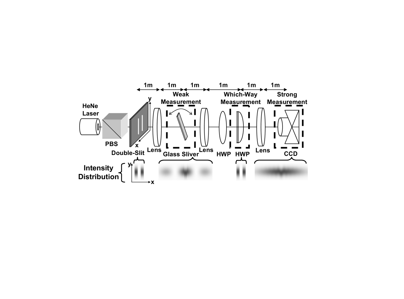
Figure 1: Diagram of apparatus. The photons are prepared in the initial state by a polarizing beam-splitter (PBS) and a double-slit aperture. They are then measured three times: the weak measurement via a $y$-displacement by the glass sliver at $p_{i}$; the which-way measurement via polarization rotation by the half-wave plate (HWP) at one slit; and the final strong measurement of $p_{f}$ by the CCD camera. For details see text. Below the apparatus are shown calculated intensity distributions at the longitudinal positions indicated, with the $y$-displacement exaggerated for clarity.

The photon ensemble is produced by a 2 $\mathrm{mW}$ $\lambda=633\mathrm{nm}$ HeNe laser that illuminates a double-slit aperture with a slit width of $w=40\mathrm{\mu m}$ and a center-to-center separation of $s=80\mathrm{\mu m}$. We call the long (vertical) axis of the slits $y$ and the axis joining their centers $x$. We use $f=1\mathrm{m}$ focal-length lenses to switch back and forth between position and momentum space for the photons. These can be treated as impulsive harmonic potentials in the classical particle picture. One metre after the first lens, the photon’s $x$-position $x_{i}$ becomes equal to $(f/c)\cdot(p_{i}/m)$, where $p_{i}$ is its initial momentum at the double-slit.Consequently, in the $x$-direction the intensity distribution is that of the expected double-slit interference pattern with a fringe spacing of $8.2\pm 0.1\mathrm{mm}$. In the $y$-direction, the intensity distribution is Gaussian with a $1/e^{2}$ half-width $\sigma=1.01\pm 0.01\mathrm{mm}.$

We tag the photons with a $y$-displacement $D$ $=$ $0.14\pm 0.01\mathrm{mm}$ ($\ll\sigma$ ensures weakness) in a range of momenta $\Delta$ centered on $p_{i}.$ This displacement is induced by tilting an optically flat glass sliver placed at $x_{i}$ with a width of $\delta=1.77\pm 0.02\mathrm{mm}$ in the $x$-direction and a thickness of $1.00\pm 0.25\mathrm{mm}$. That is, the momentum resolution of our weak measurement of $p_{i}$ is $\Delta=(m/cf)\cdot\delta\ll h/s$. If there is no momentum transfer we expect $P_{\mathrm{wv}}(p_{i}|p_{f})=1$ for $|p_{i}-p_{f}|<\Delta/2$ and $0$ otherwise. Any deviation from this represents a momentum disturbance.

To implement the WWM we must switch back to position space with a second $f=1$m lens, in essence imaging the slits.Here, the photons pass through a half-wave plate for fine alignment of their polarization.A second half-wave plate in front of the image of just one of the slits flips the polarization. That is, the photon polarization carries the WWM result, destroying the double-slit interference.Since the spatial wavefunction is unaltered, this is exactly the type of WWM Scully et al. considered.

A third $f=1$m lens transforms back into momentum space, so that finally $x_{f}=(f/c)\cdot(p_{f}/m)$. Here we record the intensity distribution with a movable CCD camera in an $x$-$y$ region of size $27.5{\mathrm{mm}}\times 2.70\mathrm{mm}.$ This was done for $x_{i}=n\delta$ for $n$ running from $-7$ to $7$.

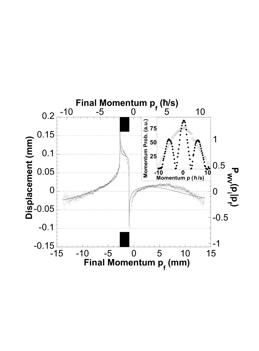
Figure 2: Weak-valued probability $P_{\mathrm{wv}}(p_{i}|p_{f})$, found from the $y$-displacement (dots) of the intensity distribution at each $p_{f}=x_{f}\cdot(mc/f)$. The thin solid curve is calculated from Eq. (4) following the theory of Ref. [19], using only the independently measured parameters, $w,s$ and $\Delta$. The solid black rectangles indicate the weak measurement window, $p_{i}\pm\Delta/2$. Here $p_{i}=-1.8\mathrm{mm}\cdot(mc/f)$, which is on the side of the central fringe. This gives rise to an asymmetric $P_{\mathrm{wv}}(p_{i}|p_{f})$, as explained in the text. The inset shows the measured intensity for each $p_{f}$ integrated over $y$, with (solid diamonds) and without (empty circles) the WWM. The intensity outside the range shown was below the sensitivity of the CCD.

The inset of Fig. 2 shows the momentum distribution of the photons at the CCD, with and without the WWM, giving $P(p_{f})$ and $P(p_{i})$ respectively. To find $P_{\mathrm{wv}}(p_{i}|p_{f})$, we measure for each $x_{f}$ the average displacement $d$ in the $y$-direction of the intensity distribution while the glass sliver is at $x_{i}$, then divide by $D$. The example in Fig. 2, for $p_{i}=-1.8$mm$\cdot(mc/f)$, shows the typical features of $P_{\mathrm{wv}}(p_{i}|p_{f})$. The dominant positive feature of the distribution coincides with the window $|p_{f}-p_{i}|\leq\Delta/2$. This reflects the fact that half the photons suffer no momentum disturbance (see the quantum eraser discussion later). The WVP is also positive when $p_{f}$ is near the minima of the initial interference pattern (see inset), as required to “fill in” these minima. Similarly, the WVP is negative when $p_{f}$ is near the maxima of the pattern. This negativity proves the existence of a nonclassical momentum disturbance. The asymmetry in the curve is because here $p_{i}$ was chosen to lie on the side of a fringe. Note that diffraction effects due to the non-zero strength of our weak measurement leads to smoothing of the experimental curve in comparison to the theory.

We sum the conditional probabilities for all fifteen $p_{i}$ according to Eq. (4) to obtain the unconditional WVP of a momentum transfer $P_{\mathrm{wv}}(q),$ plotted in Fig. 3 along with a theoretical curve. The agreement between the two is as good as we expect given the discrepancies in individual data sets exemplified in Fig. 2. Our data show that even with the WWM of the type of Scully et al., $P_{\mathrm{wv}}(q)$ is nonzero outside the range $\left[-\hbar/s,\hbar/s\right]$. This supports the stance of Storey et al. based on their theorem.

Nonetheless, theory predicts that $P_{\mathrm{wv}}(q)$ has zero variance [13], consistent with the stance of Scully et al. Unfortunately, as explained in Sec. 3, we cannot obtain the theoretical value of zero because it is practically impossible to obtain data of sufficient quality over a sufficient range of momenta to evaluate the required regularized integral [19]. Instead we calculate the integral with sharp cut-offs at $\pm q_{\max}$ (see the inset of Fig. 3). The experimental values agree qualitatively with the theoretical curve, which diverges as a function of $q_{\mathrm{max}}$. As explained in Sec. 3, it is the oscillations between positive and negative values that ensures that the theoretical prediction for the regularized integral is zero. The fact that the variance changes sign as a function of $q_{\rm max}$ demonstrates that the WWM of the type of Scully et al. does not give random momentum kicks, and is consistent with the weak-valued momentum-transfer variance being zero.

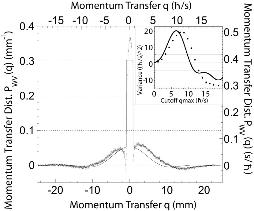
Figure 3: The weak-valued distribution for the momentum transfer $P_{\mathrm{wv}}(q)$ calculated from Eq. (1). The dots are experimental data and the thin solid line is theory as in Fig. 2. The inset is the variance integral (experiment as dots, theory as curve) over the range $[-q_{\mathrm{max}},q_{\mathrm{max}}]$ as a function of $q_{\mathrm{max}}$.

Scully et al. [6] also considered the retrieval of interference in their scheme through the use of a quantum eraser [32]. That is, interference is seen in the subsets of particles selected according to the results of projecting the apparatus in a basis conjugate to the one that carries the WWM result. For a WWM with classical momentum transfer, the different subsets give identical interference patterns apart from being shifted in the $x$-direction by varying amounts [33]. By contrast, for a WWM such as that of Scully et al., the different interference patterns all have the same envelope, but with different phases [9].

Our WWM is performed in the horizontal/vertical basis of the photon polarization, so we implement a quantum eraser using a polarizer in the $\pm 45^{\circ}$ basis. The $45^{\circ}$ photons form the usual double-slit interference pattern, whereas the $-45^{\circ}$ photons form the antiphase pattern. In Fig. 4 we plot $P_{\mathrm{wv}}(p_{i}|p_{f})$ with $p_{i}=-1.8$mm$\cdot(mc/f)$ for both polarizer settings, along with the measured interference patterns. The $45^{\circ}$ photon data show that, to a good approximation, $P_{\mathrm{wv}}(p_{i}|p_{f})=1$ if $|p_{i}-p_{f}|<\Delta/2$ and $0$ otherwise, indicating no momentum transfer. On the other hand, for the $-45^{\circ}$ photons, $P_{\mathrm{wv}}(p_{i}|p_{f})$ is substantial even for $p_{f}$ outside the range $p_{i}\pm\Delta/2$. These results are found for all values of $p_{i}$, demonstrating that the momentum transfer only appears in the photons making the antifringes. This shows an intimate connection between the nonclassical momentum transfer and the phase between the slits induced by the quantum eraser.

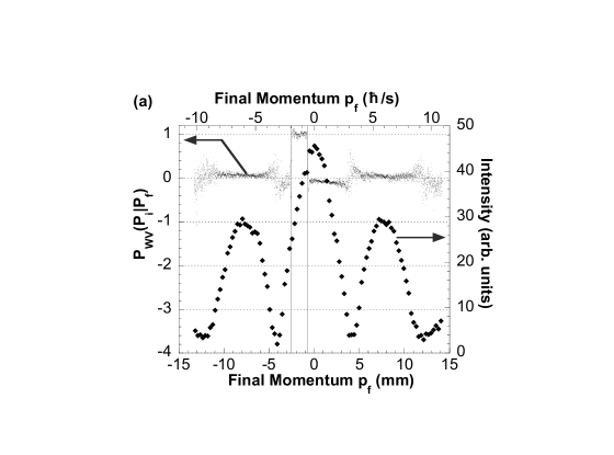
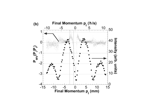
Figure 4: The WVP $P_{\rm wv}(p_{i}|p_{f})$ for $p_{i}=-1.8$mm$\cdot(mc/f)$ with a quantum eraser consisting of: a) a $45^{\circ}$ polarizer; and b) a $-45^{\circ}$ polarizer, placed after the which-way measurement. The dots indicate the $y$-displacement of the intensity distribution at each $p_{f}=x_{f}\cdot(mc/f)$ position on the CCD. The diamonds indicate the intensity at each $p_{f}$. The vertical lines indicate $p_{i}\pm\Delta/2$, the region of the weak measurement.

5 Conclusion

To conclude, we implemented a WWM of the type Scully et al. considered, and, using the technique of weak measurement, directly observed a distribution for the resultant momentum transferred. This distribution spreads well beyond $\pm\hbar/s$, in agreement with Storey et al.’s claim that complementarity is a consequence of Heisenberg’s uncertainty principle (i.e. the measurement–disturbance relation). However, the observed distribution also supports Scully et al.’s claim of no momentum transfer since its variance is consistent with zero. These seemingly contradictory observations are compatible only because the weak-valued distribution we measure takes negative values, showing the usefulness of the weak measurement technique in illuminating quantum processes.

References

References

- [1] N. Bohr, Naturwissenschaften, 16, 245 (1928).
- [2] N. Bohr, in Albert Einstein: Philosopher scientist, edited by P. A. Schlipp (Library of LivingPhilosophers, Evaston, 1949), p. 200; reprinted in Ref. [3].
- [3] Wheeler, J. A. & Zurek, W. H. (eds.) Quantum Theory and Measurement (New Jersey, Princeton, 1983).
- [4] W. Heisenberg, Zeitschrift für Physik 43, 172 (1927); translated into English in Ref. [3].
- [5] Feynman, R. P., Leighton, R. B. & Sands, M. The Feynman Lectures on Physics Vol. III (Addison Wesley, Reading MA, 1965).
- [6] M. O. Scully, B.-G. Englert, and H. Walther, Nature 351, 111 (1991).
- [7] E. P. Storey, S. M. Tan, M. J. Collett, and D. F. Walls, Nature 367, 626 (1994).
- [8] In saying that a distribution has width of at least we mean it is nonzero somewhere outside the interval .
- [9] H. M. Wiseman, F. E. Harrison, M. J. Collett, S. M. Tan, D. F. Walls, and R. B. Killip, Phys. Rev. A 56, 55 (1997).
- [10] B. G. Englert, M. O. Scully, and H. Walther, Nature 375, 367 (1995); E. P. Storey, S. M. Tan, M. J. Collett, and D. F. Walls, ibid. 375, 368 (1995).
- [11] In particular, the elegant experiment by S. Durr, T. Nonn, and G. Rempe, [Nature 395, 33 (1998)] was not relevant to this issue. As they say: “In our experiment, no double slit is used and no position measurement is performed, so that the results of Ref. [9] do not apply.”
- [12] H. M. Wiseman, F. E. Harrison, Nature 377, 584 (1995).
- [13] H. M. Wiseman, Phys. Lett. A 311, 285 (2003).
- [14] H. Weyl, Gruppentheorie und Quantenmechanik (S. Hirzel, Leipzig, 1928); translated into English by H.P. Robertson as The theory of groups and quantum mechanics (Methuen, London, 1931).
- [15] W. Heisenberg, The Physical Principles of Quantum Mechanics (The University of Chicago Press, Chicago, 1930).
- [16] H. M. Wiseman, Found. Phys. 28, 1619 (1998).
- [17] Y. Aharonov, H. Pendleton, and A. Petersen, Int. J. Theo. Phys. 2, 213–230 (1969).
- [18] Y. Aharonov, D. Z. Albert, and L. Vaidman, Phys. Rev. Lett. 60, 1351 (1988).
- [19] J. L. Garretson, H. M. Wiseman, D. T. Pope, and D. T. Pegg, J. Opt. B 6, S506 (2004).
- [20] N. W. M. Ritchie, J. G. Story, and R. G. Hulet, Phys. Rev. Lett. 66, 1107 (1991).
- [21] A. M. Steinberg, Phys. Rev. Lett. 74, 2405 (1995).
- [22] Y. Aharonov, A. Botero, S. Popescu, B. Reznik, and J. Tollaksen, Phys. Lett. A 301, 130 (2002).
- [23] K. Mølmer, Phys. Lett. A 292, 151 (2001).
- [24] H. M. Wiseman, Phys. Rev. A 65, 032111 (2002).
- [25] D. Rohrlich and Y. Aharonov, Phys. Rev. A 66, 042102 (2002).
- [26] N. Brunner, A. Acin, D. Collins, N. Gisin, and V. Scarani, Phys. Rev. Lett. 91, 180402 (2003).
- [27] D. R. Solli, C. F. McCormick, R. Y. Chiao, S. Popescu, and J. M. Hickmann, Phys. Rev. Lett. 92, 043601 (2004).
- [28] K. J. Resch, J. S. Lundeen, and A. M. Steinberg, Phys. Lett. A 324, 125 (2004).
- [29] G. J. Pryde, J. L. O’Brien, A. G. White, T. C. Ralph, and H. M. Wiseman, Phys. Rev. Lett. 94, 220405 (2005).
- [30] H. M. Wiseman, New J. Phys. 9, 165 (2007).
- [31] H. Goldstein, Classical Mechanics (Addison-Wesley, Massachussetts, 1980), 2nd edition.
- [32] M. O. Scully and K. Drühl, Phys. Rev. A 25, 2208 (1982).
- [33] W. K. Wootters and W. H. Zurek, Phys. Rev. D 19, 473 (1979).