Self-Similar Dynamics of a Magnetized Polytropic Gas

Abstract

In broad astrophysical contexts of large-scale gravitational collapses and outflows and as a basis for various further astrophysical applications, we formulate and investigate a theoretical problem of self-similar magnetohydrodynamics (MHD) for a non-rotating polytropic gas of quasi-spherical symmetry permeated by a completely random magnetic field. Within this framework, we derive two coupled nonlinear MHD ordinary differential equations (ODEs), examine properties of the magnetosonic critical curve, obtain various asymptotic and global semi-complete similarity MHD solutions, and qualify the applicability of our results. Unique to a magnetized gas cloud, a novel asymptotic MHD solution for a collapsing core is established. Physically, the similarity MHD inflow towards the central dense core proceeds in characteristic manners before the gas material eventually encounters a strong radiating MHD shock upon impact onto the central compact object. Sufficiently far away from the central core region enshrouded by such an MHD shock, we derive regular asymptotic behaviours. We study asymptotic solution behaviours in the vicinity of the magnetosonic critical curve and determine smooth MHD eigensolutions across this curve. Numerically, we construct global semi-complete similarity MHD solutions that cross the magnetosonic critical curve zero, one, and two times. For comparison, counterpart solutions in the case of an isothermal unmagnetized and magnetized gas flows are demonstrated in the present MHD framework at nearly isothermal and weakly magnetized conditions. For a polytropic index $\gamma=1.25$ or a strong magnetic field, different solution behaviours emerge. With a strong magnetic field, there exist semi-complete similarity solutions crossing the magnetosonic critical curve only once, and the MHD counterpart of expansion-wave collapse solution disappears. Also in the polytropic case of $\gamma=1.25$, we no longer observe the trend in the speed-density phase diagram of finding infinitely many matches to establish global MHD solutions that cross the magnetosonic critical curve twice.

1 Introduction

The self-similar gas dynamics in spherical symmetry involving self-gravity and thermal gas pressure has been studied over past several decades with complementary perspectives and various applications. In astrophysical and cosmological contexts, Larson (1969) and Penston (1969a, b) independently studied self-similar flow solutions in a self-gravitating gas. For modelling star formation processes in a molecular cloud and in contrast to the earlier results (Larson, 1969; Penston, 1969a, b), Shu (1977) explored self-similar collapse behaviours of an isothermal gas and obtained the central free-fall asymptotic solution and the static solution at large radii initially. Shu (1977) focused on the expansion-wave collapse solution (EWCS) by numerically joining the inner free-fall collapse solution with the outer static isothermal sphere solution (i.e., the outer part of a singular isothermal sphere). In different notations, Hunter (1977) constructed complete isothermal self-similar solutions crossing the isothermal sonic critical line once by matching solutions in the speed-density phase diagram. The variation trend of a spiral pattern in the speed-density phase diagram suggests that there may exist infinitely many discrete solutions. Hunter succeeded in connecting the two parts ($t<0$ and $t>0$ with $t$ being the time) of flows smoothly. In the same model framework, Whitworth and Summers (1985) identified and distinguished such sonic critical points as nodal and saddle points through a systematic analysis of the behaviours in the neighborhood of the isothermal sonic critical line, noted the numerical stability issue of integration directions in the vicinity of the sonic critical line, and suggested two-dimensional continua of solutions with weak discontinuities across the sonic critical line. Hunter (1986) promptly examined their continua of solutions and pointed out the weak discontinuity in their solutions (Whitworth and Summers, 1985), suggesting that these solutions may be unphysical for being unstable (see also Lazarus 1981 for more details). Moreover, Hunter (1986) proposed to use as many expansion terms as possible for a numerical integration away from nodes along the sonic critical line. Lou and Shen (2004) emphasized that the EWCS solution (Shu 1977) being static sufficiently far away only represents a special limiting case of a more general class of constant speed solutions at large $x$ and constructed global semi-complete solutions for envelope expansion with core collapse (EECC), connecting the inner free-fall asymptotic solutions with asymptotic flow solutions at large $x$ using the similar matching procedure of Hunter (1977). In particular, Lou and Shen (2004) constructed EECC solutions crossing the isothermal sonic critical line twice with radial similarity oscillations in the subsonic regime and with the divergent free-fall asymptotic behaviour in the limit of small $x$. We note in passing that steady or self-similar accretions of dark matter under self-gravity might be relevant in understanding the formation of a few recently reported supermassive black holes (SMBHs) in the early Universe (Hu et al., 2005). Lou (2005) outlined a two-fluid similarity dynamics which is fairly similar to the isothermal model mentioned above, to model the gravitational coupling between a dark matter halo and a hot interstellar gas medium. Furthermore, by incorporating a random magnetic field into the model analysis (Lou, 2005), it is possible to set up a model framework to further examine synchrotron radio emissions and magnetic Sunyaev-Zel’dovich effect in galaxy clusters (Hu and Lou, 2004). Also, the stability problem has been tackled (Ori and Piran, 1988; Hanawa and Matsumoto, 1999, 2000; Hanawa and Makayama, 1997) for the Hunter type isothermal solutions. However, because of technical issues, the free-fall solutions (Shu, 1977) remain to be analyzed in this aspect. Semelin et al. (2001) took into account of viscosity to examine the flow stability problem.

Physically, we imagine that shocks occur naturally under various astrophysical flow situations (see, e.g., Kennel and Coroniti 1984 for a model of the Crab Nebula involving MHD pulsar wind shocks and Bagchi et al. 2006 for observational evidence of MHD galaxy cluster wind shocks). In contexts of star formation, self-similar isothermal shock flows have been investigated and applied to astrophysical systems such as Bok globules and the so-called ‘champagne flows’ in H${}_{\mbox{II}}$ regions (Shu et al., 2002; Tsai and Hsu, 1995; Shen and Lou, 2004; Bian and Lou, 2005). We briefly touch upon the subject of self-similar MHD shocks here, because our MHD results (Yu and Lou, 2005) are candidate solutions for both the upstream and downstream regions across an MHD shock. The self-similar polytropic MHD shock flows will be presented elsewhere in more details (see, e.g., Yu et al., 2006 for self-similar isothermal MHD shock flows and Lou and Wang, 2007).

In polytropic MHD collapses and outflows, the polytropic index $\gamma$ represents a gross simplification from complicated physical processes including possible nuclear reactions, energy transport, neutrino transport and electron capture and so forth in various contexts (see, e.g., Bouquet et al., 1985 and Yahil, 1983). In parallel with earlier results under the isothermal approximation, the polytropic treatment has also been pursued in various astrophysical contexts including supernovae. Goldreich and Weber (1980) studied the $\gamma=4/3$ case with a focus on the homologous collapse of the inner core of a progenitor star prior to the emergence of a rebound shock (e.g., Lou and Wang, 2006, 2007). Yahil (1983) noted limitations of Goldreich-Weber model, studied the polytropic gas dynamics within the polytropic index range of $6/5\leq\gamma\leq 4/3$, and discussed possible applications to the pre-catastrophe as well as post-catastrophe phases separately. A few years earlier, Cheng (1978) investigated the polytropic hydrodynamics with $1\leq\gamma\leq 5/3$, focussing on the initial distribution of mass density $\rho$ with a radial scaling of $\rho\sim r^{\alpha}$. For a polytropic gas, Cheng (1978) derived the inner free-fall solution and generalized the isothermal EWCS to the polytropic EWCS. Bouquet et al. (1985) introduced a dual space of parameters as well as the systems I and II for the polytropic gas dynamics with $1\leq\gamma\leq 4/3$, and analyzed properties of the sonic critical curve in details. Suto and Silk (1988) performed a similarity transformation for the polytropic gas dynamics and, from the resulting nonlinear ordinary differential equations (ODEs), obtained regular and asymptotic solutions as well as numerical solutions with $n=1$ and $\gamma=2-n$ for $1<\gamma<4/3$. By taking into account of the total radiative emissivity from the gas in the form of $\epsilon\sim\rho^{\alpha}T^{4+\beta}$, Boily and Lynden-Bell (1995) replaced the polytropic equation of state with an energy equation and discussed physical, mathematical and numerical properties of such radiative self-similar gas dynamics. McLaughlin and Pudritz (1997) considered the limiting case of the so-called logotropic gas dynamics also involving sonic critical points and obtained expansion-wave collapse solutions in their analysis. In the context of star formation, Fatuzzo et al. (2004) studied a combination or a transition of an initial ‘equation of state’ $P\propto\rho^{\Gamma}$ and a later dynamic equation of state $P\propto\rho^{\gamma}$, and noted that in the special case of $\Gamma=1$, asymptotic solutions may have constant flow speed at far away regions, analogous to the earlier results of Lou and Shen (2004) and Shen and Lou (2004). Fatuzzo et al. (2004) carried out their analysis for the case of $\gamma<1$ without involving the sonic critical curve.

Magnetic field can be extremely important in many astrophysical processes on different scales and in particular, for star formation activities at various stages (e.g., Shu et al., 1987). In mostly neutral gas medium, such as molecular clouds and cores etc., the magnetic field can only couple to the gas medium if MHD wave frequencies are less than the ion-neutral collision frequency, corresponding to a lower limit on the wavelength that MHD waves need in order to propagate in such a magnetized cloud (e.g., Myers, 1998). At the end of stellar evolution, magnetic fields are observed to exist in various stellar systems such as the well-known Crab Nebula (e.g., Woltjer, 1957, 1958a, b; Kennel and Coroniti, 1984a, b; Wilson et al., 1985; Lou, 1993; Wolf et al., 2003). Chiueh and Chou (1994) discussed the gravitational collapse of an isothermal magnetized gas cloud, including the magnetic pressure force term in the radial momentum equation together with the magnetic induction equation. They assumed a randomly distributed magnetic field such that a quasi-spherical symmetry is sustained during the MHD similarity evolution of a gas cloud on large scales. Magnetic tension force was ignored in their formulation. Yu and Lou (2005) approached the same physical problem yet with a different formulation and discussed MHD consequences of a random magnetic field. Using the frozen-in condition on magnetic field, Yu and Lou (2005) managed to reduce the three apparently coupled nonlinear MHD equations to two key coupled nonlinear MHD ODEs in an equivalent manner. Yu et al. (2006) further explored various self-similar isothermal MHD shocks under the approximation of large-scale quasi-spherical symmetry.

Self-similar gas dynamics for stellar collapse problems under self-gravity and thermal pressure have been studied extensively from various perspectives. In this paper, we construct similarity MHD solutions to explore nonlinear effects of a random magnetic field. In general, MHD similarity collapses and outflows evolve nonlinearly by simply changing certain profile scalings of the enclosed mass, gas mass density, radial flow speed, and mean transverse magnetic field energy density without changing their shapes. Hydrodynamic simulations have pointed to possible similarity evolutions as all sorts of transients peter out in time (see, e.g., Bodenheimer and Sweigart, 1968 and Foster and Chevalier, 1993). The well-known example is the Sedov-Taylor similarity blast waves resulting from a point explosion (Sedov, 1959; Landau and Lifshitz, 1959; Barenblatt and Zel’dovich, 1972). Self-similar flow solutions have been explored in different geometries (Fillmore and Goldreich, 1984; Hennebelle, 2003; Terebey et al., 1984; Inutsuka and Miyama, 1992; Shadmehri, 2005; Krasnopolsky and Königl, 2002; Shen and Lou, 2006) and we here work with the quasi-spherical geometry mainly by a more phenomenological consideration. For the example of the Crab Nebula projected onto the plane of the sky, a quasi-spherical morphology (more or less elliptical in reality) has been sustained on large scales. Another example is the Cassiopeia A supernova remnant (resulting from a type II supernova explosion presumably) which, projected onto the plane of sky, appears more or less round with a central neutron star manifested as a bright X-ray point. There are also examples of more or less round planetary nebula systems where magnetic fields, be they weak or strong, are also likely involved. We invoke these morphological examples involving magnetic fields to justify an MHD collapse and expansion problem with a quasi-spherical symmetry on large scales as a first approximation. We also assume that small-scale deviations from the quasi-spherical symmetry is relatively insignificant in large-scale MHD, i.e., small-scale transverse flow components are random and may be neglected to simplify the mathematical treatment. Since magnetic field strengths can be significant in various astrophysical systems (Yu and Lou, 2005), we should take into account of the MHD influence in the evolution of a magnetized gas cloud or a magnetized star (Lou, 1993, 1994) as well as MHD gas systems on much larger scales.

For a random magnetic field in a cloud, we envision a simple ‘ball of thread’ scenario in a vast spatial volume of gas medium. A magnetic field line follows the ‘thread’ meandering within a thin spherical ‘layer’ in space in a random manner. In the strict sense, there is always a random weak radial magnetic field component such that random magnetic field lines in adjacent ‘layers’ are actually connected throughout in space. By taking a large-scale ensemble average of such a magnetized gas system, we are then left with ‘layers’ of random magnetic field components transverse to the radial direction. Having gone thus far in our idealization, we would admit that the magnetic fields in the Crab Nebula, the SNR Cas A as well as several round planetary nebulae may not be fully represented by of “ball of thread” scenario. What we have been trying to emphasize is the large-scale quasi-spherical geometry of magnetized astrophysical systems rather than detailed magnetic field configurations. We note also that, in our model, the “ball of thread” scenario is mainly for the transverse magnetic field effect on average, while the MHD effect of a weak radial magnetic field may be negligible. As a matter of fact, we will still need further observational information to infer whether our magnetic field configuration can roughly describe some round-shaped morphologies of astrophysical systems.

In reference to the recent isothermal self-similar MHD analysis (Yu and Lou, 2005), we show in this paper that an isothermal similarity MHD treatment can be naturally extended to a magnetized polytropic gas in a systematic manner. Parallel to the self-similar transformation for relevant variables (Suto and Silk, 1988) with an additional transformation for the transverse magnetic field, we derive three apparently coupled nonlinear MHD ODEs, as in the case of an isothermal magnetofluid (Chiueh and Chou, 1994). The major technical difference in our polytropic MHD formalism is that these three ODEs can be readily reduced to two key ODEs of MHD by invoking the frozen-in condition on magnetic field (Yu et al., 2006; Lou & Wang, 2007). This frozen-in condition (21) naturally leads to an integration constant $h$ denoting physically the ratio of the magnetic energy density to the self-gravitational energy density and significantly reduces the complexity of analyzing the nonlinear similarity MHD problem. Although only a change of equation of state is made in our current formulation as compared to the isothermal treatment (Yu and Lou, 2005), several distinct differences arise. For example, the magnetosonic critical curve now shows qualitatively different asymptotic behaviours as compared to an isothermal gas, both in unmagnetized and magnetized cases (Lou and Wang, 2006, 2007). By increasing the polytropic index $\gamma$, we find qualitative differences in reference to the case of a smaller $\gamma$. Most importantly, we found a novel asymptotic nonlinear MHD solution near the central core or at later time and constructed semi-complete MHD similarity solutions using this asymptotic solution. We have also discovered the so-called ‘quasi-static’ asymptotic polytropic MHD solution behaviours (see Lou and Wang, 2006 for polytropic hydrodynamic asymptotic solutions). We here focus on the MHD case and provide a description in Appendix G. A more detailed analysis and astrophysical applications of this MHD asymptotic solution can be found in Lou and Wang (2007).

Motivated by potentially wide astrophysical applications, the main purpose of this paper is to present possible similarity solutions from the nonlinear MHD ODEs, distinguish the asymptotic behaviours of different types including the eigensolutions across the magnetosonic critical curve, and construct global semi-complete solutions numerically. Our analyses and results here serve as the theoretical basis for further specific astrophysical MHD applications. We provide the background information in Section 1 as an introduction. Section 2 contains the basic MHD formulation of the problem and section 3 presents the mathematical analysis. Section 4 mainly describes numerical results, including the magnetosonic critical curves, similarity MHD solutions without crossing the magnetosonic critical curve, similarity solutions crossing the magnetosonic critical curve once and twice. In both analytical and numerical analyses, we focus on differences between the cases with or without magnetic field and between weak and strong magnetic field. We also compare the case in which $\gamma$ is almost unity to that in which $\gamma$ is larger than one, and further discuss differences between a nearly isothermal polytropic gas and an exact isothermal case.

2 Similarity MHD Flows

In this section, the basic MHD formulation of the similarity problem is presented and the approximation of quasi-spherical symmetry is discussed (Appendix A).

2.1 MHD Formulation of the Problem

Under the assumptions of a random magnetic field on smaller scales, the approximation of quasi-spherical symmetry and the ideal MHD treatment, the dynamics of a polytropic magnetized gas in spherical polar coordinates $(r,\theta,\phi)$ is described by the following equations:

$$\frac{\partial\rho}{\partial t}+\frac{1}{r^{2}}\frac{\partial}{\partial r}(r^{2}\rho u)=0\ ,$$ (1)

$$\frac{\partial M}{\partial t}+u\frac{\partial M}{\partial r}=0\ ,$$ (2)

$$\frac{\partial M}{\partial r}=4\pi r^{2}\rho\ ,$$ (3)

$$\rho\bigg{(}\frac{\partial u}{\partial t}+u\frac{\partial u}{\partial r}\bigg{)} = -\frac{\partial p}{\partial r}-\frac{GM\rho}{r^{2}}$$ (4)

$$-\frac{\partial}{\partial r}\bigg{(}\frac{<B_{t}^{2}>}{8\pi}\bigg{)}-\frac{<B_{t}^{2}>}{4\pi r}\ ,$$

$$\frac{\partial}{\partial t}\big{(}r^{2}<B_{t}^{2}>\big{)} + u\frac{\partial}{\partial r}\big{(}r^{2}<B_{t}^{2}>\big{)}$$ (5)

$$+ 2r^{2}<B_{t}^{2}>\frac{\partial u}{\partial r}=0\ ,$$

$$p=\kappa\rho^{\gamma}\ ,$$ (6)

where $G=6.67\times 10^{-8}\hbox{ g}^{-1}\hbox{ cm}^{-3}\hbox{ s}^{-2}$ is the gravitational constant, $\rho(r,t)$ is the gas mass density, $M(r,t)$ is the enclosed gas mass within radius $r$ at time $t$, $u(r,t)$ is the bulk radial flow speed, and $<B_{t}^{2}>$ is the mean square of the random transverse magnetic field $\vec{B}_{t}$ proportional to the magnetic energy density associated with the random transverse magnetic field. In the conventional polytropic equation of state (6), the coefficient $\kappa$ remains constant globally, independent of both $r$ and $t$. The case of $\gamma=1$ is only a special case corresponding to an isothermal magnetized gas (Yu and Lou, 2005; Yu et al., 2006). The Poisson equation relating the mass density and the gravitational potential is automatically satisfied under the quasi-spherical symmetry. In the above equations, the radial momentum equation (4) involves the magnetic pressure and tension forces on the right-hand side (RHS), and equation (5) is derived from the magnetic induction equation along with certain simplifications (Yu and Lou, 2005); these two equations will be further discussed and analyzed in the next subsection. Compared to the work of Chiueh and Chou (1994), the formulation here is different by keeping the magnetic tension force and by dealing with a conventional polytropic gas. For the problem outlined above, the reader may consult relevant references (Shu 1977; Suto and Silk, 1988; Chiueh and Chou, 1994; Lou and Shen, 2004; Bian and Lou, 2005; Yu and Lou, 2005; Yu et al., 2006; Lou & Wang, 2006, 2007). We focus on the semi-complete solution space $0<t<+\infty$ rather than the complete solution space as introduced by Hunter (1977).

For a conventional polytropic gas with $\gamma=2-n$ where $\gamma$ and $n$ are defined by equations (15) and (3.1), respectively (see subsection 3.1), a combination of equations (1)$-$(5) together with equation (15) leads to the MHD energy conservation equation as

$$\frac{\partial}{\partial t}\bigg{[}\frac{\rho u^{2}}{2} + \frac{p}{(\gamma-1)}-\frac{1}{8\pi G}\left(\frac{\partial\Phi}{\partial r}\right)^{2}+\frac{<B_{t}^{2}>}{(8\pi)}\bigg{]}$$ (7)

$$+ \frac{1}{r^{2}}\frac{\partial}{\partial r}\bigg{\{}r^{2}u\rho\bigg{[}\frac{u^{2}}{2}+\frac{\gamma p}{(\gamma-1)\rho}\bigg{]}\bigg{\}}$$

$$+ \frac{1}{r^{2}}\frac{\partial}{\partial r}\bigg{(}r^{2}u\rho\Phi+\frac{r^{2}\Phi}{4\pi G}\frac{\partial^{2}\Phi}{\partial r\partial t}\bigg{)}$$

$$+ \frac{1}{r^{2}}\frac{\partial}{\partial r}\bigg{(}\frac{r^{2}u}{4\pi}<B_{t}^{2}>\bigg{)}=0\ ,$$

where $-\partial\Phi/\partial r=-GM/r^{2}$ and $\Phi$ is the gravitational potential (Fan and Lou, 1999). This MHD energy conservation equation reduces to the isothermal cases (Lou and Shen, 2004; Yu and Lou, 2005) by taking the L’H$\hat{\mbox{o}}$pital rule with respect to $\gamma$ in the limit of $\gamma\rightarrow 1$. The magnetic energy density and Poynting flux density associated with $<B_{t}^{2}>$ can be readily identified in the MHD energy conservation equation (7). With the quasi-spherical symmetry, the divergence term containing $\Phi$ in MHD energy conservation equation (7) vanishes (Lou and Shen, 2004).

2.2 Comments on the MHD Formalism

We here briefly comment on the basic MHD formulation, the quasi-spherical symmetry, the three-dimensional random flow fluctuations on small scales and the physical basis for the magnetic force density and the magnetic induction equation.

Our MHD model describes a self-gravitating gas cloud embedded with a magnetic field presumed to be random and tangled on small scales. On large scales, the gas mass density, the gas thermal temperature, the thermal pressure and the entropy are all taken to be quasi-spherically symmetric. The magnetic field distribution is presumed to be completely random in space such that in a small volume (an infinitesimal volume $r^{2}\text{d}r\text{d}\theta\text{d}\phi$) the magnetic field is effectively represented by the mean square averages of $<B_{r}^{2}>$ and $<B_{t}^{2}>$, proportional to the radial and transverse magnetic energy densities respectively. In terms of the magnetic pressure and tension forces for the large-scale MHD, $<B_{t}^{2}>$ plays the dominant role on the dynamics of a magnetized gas cloud as compared to $<B_{r}^{2}>$. As the magnetic field is randomly distributed with a quasi-spherical symmetry, the bulk gas flow velocity remains grossly spherically symmetric and can be characterized by the bulk mean radial flow speed $v_{r}$; the transverse component of the flow velocity $v_{\theta}$ and $v_{\phi}$ are relatively small and may be neglected in the first approximation. These transverse components should be part of Alfvénic fluctuations corresponding to magnetic field fluctuations about the mean configuration; thus the more random the magnetic field fluctuations are, the better the approximation becomes.

The physical concept of a quasi-spherical symmetry for a magnetized gas cloud or a magnetized progenitor star is only valid for MHD processes of sufficiently large scales. Here, ‘large scales’ are obviously in contrast to ‘small scales’ on which magnetic fields are presumed completely random locally in our MHD model framework. In the strict sense, an exact spherical symmetry is impossible due to the very nature of a magnetic field. However, a quasi-spherical symmetry may be sustained for large-scale MHD processes. We invoke the projected quasi-elliptical shape of the Crab Nebula and the projected more or less round remnant of the Cassiopeia A supernova as empirical supports for this notion of quasi-spherical symmetry. Although it is not yet obvious that the actual magnetic field can be largely approximated by our ‘ball of thread’ scenario, from the morphology of these systems we suggest a globally random magnetic field distribution as a plausible yet tractable starting point. In this scenario, small-scale random flow velocities are ignored as compared to systematic radial flows. Qualitatively speaking, this perspective is justifiable when a random magnetic field is weak. In our model analysis, we sometimes do encounter situations of strong magnetic fields especially for accretions towards a central compact object. In such a case, one should really view our asymptotic MHD solutions as indicating a gross trend of variation that is bound to be destroyed by non-spherical and transient MHD processes sufficiently close to the central compact object. Upon impacting onto a central compact object, we expect the emergence of a strong radiating MHD shock traveling outward slowly in a self-similar manner (Shen and Lou, 2004; Yu and Lou, 2005; Yu et al., 2006). Practically, we can apply our large-scale self-similar MHD solutions of quasi-spherical symmetry outside this radiating MHD shock. Within this quasi-spherical MHD shock, the core gravity can be strong enough to more or less hold on the strongly magnetized plasma. By the naïve solar analogy, we readily imagine that sporadic violent ‘flares’ or ‘coronal mass ejections’ may erupt from the strongly magnetized central core region and can even break into the ‘self-similar’ and ‘quasi-spherical’ domain of magnetized accreting flows.

Given local random magnetic fields on small scales in a gas medium, three-dimensional MHD flows on small scales are naturally expected because of the unbalanced magnetic tension force here and there. Except for very special self-similar radial flow situations of zero transverse flows yet with a three-dimensional magnetic field (see Low 1992), we do generally expect small-scale three-dimensional random flow fluctuations associated with the large-scale mean radial flow. By our assumption of a randomly tangled magnetic field, such flow fluctuations are more or less confined or trapped locally and advected by the mean radial MHD flow on large scales. In short, we do not expect mean flows transverse to the radial direction on large scales in our scenario. By intuition, we expect transverse flows caused by the random magnetic tension force, yet such flows will remain locally confined due to the local random magnetic field and hence be small as compared with the bulk quasi-spherical radial flow speed. As suggested by Zel’dovich and Novikov (1971), an isotropic magnetic pressure is expected from a completely random magnetic field on small scales. We follow this basic concept and also include the radial magnetic tension force which is non-negligible in our formulation. Physically, one may view such small-scale random flow fluctuations as turbulence and for simplicity, we have ignored the effects of the effective turbulent pressure, viscosity and resistivity etc. (see, e.g., Lou and Rosner, 1986) in this formulation. In our model framework, if the MHD turbulence will attribute to random fields and fluctuations on smaller scales, the turbulence scale itself should be small enough such that the largest turbulence scale is small compared to the overall quasi-spherical geometry.

3 Model Analysis

With the basic ideal MHD model qualified and the formulation established, we now perform the analytical and numerical analyses in order. In the next section, we present the results of numerical exploration.

3.1 Self-Similar MHD Processes in a
Magnetized Polytropic Gas Cloud

To seek self-similar solutions to the MHD equations, we introduce an independent similarity dimensionless variable $x$ and presume that dependent physical variables are given by the following similarity forms accordingly:

$$r=ax,u=bv,\rho=c\alpha,p=d\beta,M=em,<B_{t}^{2}>=fw\ ,$$ (8)

where the six scaling factors $a(t)$ through $f(t)$ are functions of time $t$ only and are defined by

$$a\equiv k^{1/2}t^{n}\ ,\qquad b\equiv k^{1/2}t^{n-1}\ ,\qquad c\equiv\frac{1}{4\pi Gt^{2}}\ ,\qquad$$

$$d\equiv\frac{kt^{2n-4}}{4\pi G}\ ,\quad e\equiv\frac{k^{3/2}t^{3n-2}}{(3n-2)G}\ ,\quad f\equiv\frac{kt^{2n-4}}{G}\ .$$ (9)

Here $k$ and $n$ are two constant parameters. As functions of $x$ only, $v(x)$, $\alpha(x)$, $\beta(x)$, $m(x)$, and $w(x)$ are the reduced forms of radial flow speed, gas mass density, gas pressure, enclosed gas mass, and magnetic energy density (associated with the averaged random transverse magnetic field), respectively. With this self-similar MHD transformation, equations (2) and (3) lead to an algebraic expression for $m(x)$ in terms of $\alpha(x)$ and $v(x)$, viz.

$$m=\alpha x^{2}(nx-v)\ ,$$ (10)

and an ODE for $\alpha(x)$ and $v(x)$

$$(nx-v)\alpha^{\prime}-\alpha v^{\prime}=-2\frac{(x-v)}{x}\alpha\ ,$$ (11)

where the prime ^′ denotes the differentiation with respect to $x$. Relation (10) leads to the important inequality

$$nx-v>0\$$ (12)

for a positive gas mass density as noted repeatedly in figure displays presently. In our later analyses, this inequality is a key constraint on choosing relevant physical solutions. From equation (5), one obtains

$$(nx-v)w^{\prime}-2wv^{\prime}=\frac{2v-(4-2n)x}{x}w\$$ (13)

for the reduced dependent variables $w(x)$ and $v(x)$. This constraint for the reduced magnetic energy density is fairly similar to equation (11). By equation (4), one obtains the reduced radial momentum equation

$$\frac{\beta^{\prime}}{\alpha}-(nx-v)v^{\prime}+\frac{w^{\prime}}{2\alpha}=-(n-1)v-\frac{w}{x\alpha}-\frac{nx-v}{3n-2}\alpha\ .$$ (14)

For a generalized polytropic equation of state with a polytropic index $\gamma$ (Suto and Silk, 1988), we simply have

$$\beta=\alpha^{\gamma},\qquad p=k(4\pi G)^{\gamma-1}t^{2(n+\gamma-2)}\rho^{\gamma}=\kappa\rho^{\gamma}\ ,$$ (15)

where $\kappa$ may be time dependent in general. For $n=2-\gamma$, we have a constant $\kappa=k(4\pi G)^{\gamma-1}$ and equation (15) is an equation of state for a conventional polytropic gas.

A combination of equations (14) and (15) leads to

$$\gamma\alpha^{\gamma-2}\alpha^{\prime}-(nx-v)v^{\prime}+\frac{w^{\prime}}{2\alpha}$$

$$=-(n-1)v-\frac{w}{x\alpha}-\frac{(nx-v)}{(3n-2)}\alpha\ ,$$ (16)

and equations (11), (13) and (3.1) are the three MHD similarity ODEs describing polytropic magnetized gas flows with a quasi-spherical symmetry. The three nonlinear MHD ODEs are similar to those of Chiueh and Chou (1994) with the key differences in the adopted equation of state and in keeping the magnetic tension force term (see equations 1 to 5). By taking relevant limits as necessary checks, these equations are consistent with those of Shu (1977), Suto and Silk (1988), Lou and Shen (2004), Yu and Lou (2005), Yu et al. (2006), Lou and Wang (2006, 2007) as expected.

The Alfvén speed in this formulation is defined by

$$v_{A}\equiv\left(\frac{<B_{t}^{2}>}{4\pi\rho}\right)^{1/2}\ ,$$ (17)

and the sound speed $s$ in the polytropic gas determined by the equation of state with $\gamma=2-n$ (i.e., the polytropic state equation in the usual sense) is simply

$$s\equiv\bigg{(}\frac{\partial p}{\partial\rho}\bigg{)}^{1/2}\ .$$ (18)

Thus the ratio of the Alfvén wave speed to the polytropic sound speed becomes

$$\frac{v_{A}}{s}=\bigg{(}\frac{w}{\gamma\alpha^{\gamma}}\bigg{)}^{1/2}\ ,$$ (19)

consistent with the isothermal $\gamma=1$ case (Yu and Lou, 2005; Yu et al., 2006).

3.2 Reduction of Nonlinear MHD ODEs

One can readily reduce the three coupled nonlinear MHD ODEs to two. From equation (11), one obtains

$$\frac{\alpha^{\prime}}{\alpha}=\frac{v^{\prime}-2(x-v)/x}{nx-v}\ ,$$

and from equation (13), one gets

$$\frac{w^{\prime}}{w}=\frac{2v^{\prime}+2[2v-(4-2n)x]/x}{nx-v}\ .$$

The above two equations lead to a differential relation

$$\frac{w^{\prime}}{w}=\frac{2\alpha^{\prime}}{\alpha}+\frac{2}{x}\ ,$$ (20)

which immediately gives a simple integral of

$$w=h\alpha^{2}x^{2}\ ,$$ (21)

where $h$ is an integration constant providing a measure for the magnetic field strength. Integral (21) gives a new parameter $h$ of a magnetized gas cloud besides $n$ and $\gamma$, and reduces the three coupled nonlinear MHD ODEs to two. Expressed explicitly in physical quantities, $h$ is

$$h=\frac{<B_{t}^{2}>}{16\pi^{2}G\rho^{2}r^{2}}\ ,$$

representing the ratio of the magnetic energy density to the self-gravitational energy density. This simplification reduces tremendously complications in numerical MHD exploration and physically represents the frozen-in condition on magnetic field (Yu and Lou, 2005; Yu et al., 2006). The procedure of numerically constructing global MHD solutions and matching the solutions across the magnetosonic critical curve can be carried out similar to that of Lou and Shen (2004). This reduction of three coupled nonlinear MHD ODEs to two is parallel to the isothermal case (Yu and Lou, 2005; Yu et al., 2006).

Substitution of equation (21) into equation (3.1) gives

$$(\gamma\alpha^{\gamma-2} + hx^{2})\alpha^{\prime}-(nx-v)v^{\prime}$$ (22)

$$= -(n-1)v-\bigg{(}2hx+\frac{nx-v}{3n-2}\bigg{)}\alpha\ .$$

Equations (11) and (22) together lead to the two coupled nonlinear MHD ODEs in the forms of

$$\alpha^{\prime}=\alpha^{2}\bigg{[}(n\!\! - \!\!1)v+\bigg{(}2hx+\frac{nx-v}{3n-2}\bigg{)}\alpha$$

$$-\frac{2(x-v)(nx-v)}{x}\bigg{]}\!\!\!\! \bigg{/} \!\!\!\!\bigg{[}\alpha(nx-v)^{2}-\gamma\alpha^{\gamma}-h\alpha^{2}x^{2}\bigg{]}\ ,$$

$$v^{\prime}=\bigg{\{}(n-1)\big{[}\alpha v(nx-v)+2h\alpha^{2}x^{2}\big{]}+\frac{(nx-v)^{2}}{(3n-2)}\alpha^{2}$$

$$\quad-2\gamma\alpha^{\gamma}\frac{(x-v)}{x}\bigg{\}}\bigg{/}\bigg{[}\alpha(nx-v)^{2}-\gamma\alpha^{\gamma}-h\alpha^{2}x^{2}\bigg{]}\ .$$ (24)

We now introduce simplifying notations as follows

$$A(\alpha,v,x)\equiv\alpha^{2}\bigg{[}(n-1)v\qquad$$

$$\quad+\bigg{(}2hx+\frac{nx-v}{3n-2}\bigg{)}\alpha-2\frac{(x-v)(nx-v)}{x}\bigg{]}\ ,\qquad\quad$$ (25)

$$V(\alpha,v,x)\equiv(n-1)\big{[}\alpha v(nx-v)+2h\alpha^{2}x^{2}\big{]}\qquad\qquad$$

$$\qquad+\frac{(nx-v)^{2}}{(3n-2)}\alpha^{2}-2\gamma\alpha^{\gamma}\frac{(x-v)}{x}\ ,$$ (26)

$$X(\alpha,v,x)\equiv\alpha(nx-v)^{2}-\gamma\alpha^{\gamma}-h\alpha^{2}x^{2}\ ,$$ (27)

to transform equations (3.2) and (24) into

$$\frac{\text{d}x}{X(\alpha,v,x)}=\frac{\text{d}\alpha}{A(\alpha,v,x)}=\frac{\text{d}v}{V(\alpha,v,x)}=\text{d}\xi\ ,$$ (28)

where $\xi$ is a new dependent variable.

The two coupled nonlinear MHD ODEs (3.2) and (24) are analyzed to determine the magnetosonic critical curve and asymptotic solution behaviours near the magnetosonic critical curve, and can be integrated numerically using the standard fourth-order Runge-Kutta scheme (e.g., Press et al., 1986). Along with the similarity MHD transformation, these two coupled nonlinear MHD ODEs describe an important subset of MHD solutions to the original nonlinear partial differential MHD equations (1)$-$(5).

Using the above simplification, the ratio of Alfvén wave speed $v_{A}$ to the gas sound speed $s$ becomes

$${v_{A}}/{s}=(h\alpha^{2-\gamma}x^{2}/\gamma)^{1/2}\$$ (29)

for $\gamma+n=2$.

3.3 Singular Surface and Magnetosonic Critical Curve

Given parameters $n$, $\gamma$ and $h$ in MHD ODEs (3.2) and (24), there exists a characteristic surface in the $(v,\alpha,x)$ space on which the denominators on the RHSs of both equations vanish (Whitworth and Summers, 1985). Physically, we have averaged over small-scale MHD fluctuations in our formulation. Therefore, the magnetosonic critical point or curve should correspond to a layer of a thickness comparable the mean scale of MHD fluctuations. In other words, our model analysis relates to an averaged condition in the actual MHD flow. Mathematically, this singular surface is determined by computing $v$ from specific $x$ and $\alpha$ in the ranges of $0<x<+\infty$ and $0<\alpha<+\infty$, namely,

$$v=nx\mp(\gamma\alpha^{\gamma-1}+h\alpha x^{2})^{1/2}\ ,$$ (30)

in which one should pick up the upper minus sign in order to satisfy the physical constraint of $nx>v$ and thus to ensure $m(x)>0$. The solutions of the two coupled ODEs (3.2) and (24) cannot cross the singular surface unless they cross it at points along the so-called magnetosonic critical curve where both the numerators and denominators vanish simultaneously. Along this magnetosonic critical curve, the derivatives of the dependent variables $v(x)$ and $\alpha(x)$ can be calculated from equations (3.2) and (24) using the L’H$\hat{\mbox{o}}$pital rule. Mathematically, this magnetosonic critical curve is defined by the following pair of equations

$$(nx-v)^{2}=\gamma\alpha^{\gamma-1}+h\alpha x^{2}\$$ (31)

and

$$(n-1)v+\bigg{(}2hx+\frac{nx-v}{3n-2}\bigg{)}\alpha-\frac{2(x-v)(nx-v)}{x}=0;$$ (32)

these two equations immediately give

$$v=nx\mp(\gamma\alpha^{\gamma-1}+h\alpha x^{2})^{1/2}\ ,$$

$$\pm\bigg{[}n-1 + \frac{\alpha}{(3n-2)}\bigg{]}(\gamma\alpha^{\gamma-1}+h\alpha x^{2})^{1/2}\qquad\qquad$$ (33)

$$\qquad\ =\frac{2\gamma}{x}\alpha^{\gamma-1}-n(n-1)x\ ,$$

with the latter leading to a quadratic equation of $x^{2}$ as

$$A_{1}x^{4}+B_{1}x^{2}+C_{1}=0\ ,$$ (34)

where the coefficients $A_{1}$, $B_{1}$ and $C_{1}$ are defined by

$$A_{1}\equiv\bigg{[}n-1+\frac{\alpha}{(3n-2)}\bigg{]}^{2}h\alpha-n^{2}(n-1)^{2}\ ,$$

$$B_{1}\equiv\gamma\alpha^{(\gamma-1)}\left\{\bigg{[}n-1+\frac{\alpha}{(3n-2)}\bigg{]}^{2}+4n(n-1)\right\}\ ,$$

$$C_{1}\equiv-4\gamma^{2}\alpha^{(2\gamma-2)}\ .$$ (35)

If one substitutes equations (32) and (33) into equation (24), the numerator vanishes. By the physical constraint of $m(x)>0$, the lower minus sign in equation (33) will be ignored, even though mathematically, it may represent a new branch of the critical curve should this branch do exist. The above expressions of the magnetosonic critical curve appear far more complicated than the isothermal case (Shu, 1977; Lou and Shen, 2004; Yu and Lou, 2005; Yu et al., 2006; Lou and Gao, 2006), as a result of a polytropic gas under the influence of a random magnetic field characterized by a constant $h$ and a reduced magnetic energy density $w(x)$. In reference to earlier results of determining $v(x)$ and $\alpha(x)$ in terms of $x$ along the critical curve, the most straightforward procedure one can take in the current polytropic MHD problem is to first determine $x$ from a given $\alpha$ and then obtain the corresponding $v$. This is somewhat unusual in determining the magnetosonic critical curve for a given sequence of $\alpha$ values. The additional constraints for the magnetosonic critical curve in the semi-complete space are $x>0$ and $\alpha>0$ besides equation (34). Physically, we are interested in the parameter regime of $nx-v>0$ such that $m(x)>0$. It is obvious that we always have $C_{1}<0$ in definition (35). For different $\alpha$ values and depending on the values of coefficients $A_{1}$, $B_{1}$ and $C_{1}$, there are three possible cases listed below.

Case I: subcase (i) of both $A_{1}<0$ and $B_{1}<0$ or subcase (ii) a negative determinant $B_{1}^{2}-4A_{1}C_{1}<0$; there is then no positive root for $x^{2}$ satisfying quadratic equation (34) and therefore there is no point along the magnetosonic critical curve corresponding to such a range of $\alpha$ values.

Case II: with $A_{1}<0$, $B_{1}>0$ and a non-negative determinant $B_{1}^{2}-4A_{1}C_{1}\geq 0$, there are two positive roots for $x^{2}$ satisfying quadratic equation (34); there are thus two points on the magnetosonic critical curve corresponding to such a range of $\alpha$ values.

Case III: with $A_{1}>0$, there is only one positive root for $x^{2}$ satisfying quadratic equation (34) and there is thus one point on the magnetosonic critical curve corresponding to such a range of $\alpha$ values.

Once an $x$ value is determined for a given $\alpha>0$ by the above procedure, we readily obtain the corresponding $v$ value. According to equation (33) for

$$\frac{2\gamma\alpha^{\gamma-1}/x-n(n-1)x}{[n-1+\alpha/(3n-2)]}>0\ ,$$ (36)

we should obviously pick up the upper sign (i.e., the ${}^{\prime}+^{\prime}$ sign in the second relation and ${}^{\prime}-^{\prime}$ sign in the first relation) in equation (33); otherwise, we should pick up the other sign accordingly. As the physical constraint $m(x)>0$ requires that $nx-v>0$, inequality (36) sets the criterion for a physical solution.

This sequence of determining the magnetosonic critical curve appears more involved than those in the isothermal case without a random magnetic field (Shu, 1977; Lou and Shen, 2004).

3.4 Asymptotic and Global Similarity Solutions

In order to specify initial or boundary conditions for numerical integrations, one needs to derive asymptotic similarity MHD solutions. These asymptotic MHD solutions also carry their physical implications. It is also possible to derive some regular solutions from the coupled nonlinear MHD ODEs for physical interpretations and for reference of numerical results. In general, we have found the MHD counterparts of the isothermal asymptotic solutions (Lou and Shen, 2004), and, in particular, we have derived a novel MHD asymptotic solution as well as a new class of asymptotic behaviours. We also examine the corresponding ratio of the Alfvén wave speed to the sound speed and the dominant force among the gravity force, the thermal pressure gradient force, the magnetic pressure gradient force and the magnetic tension force for each MHD asymptotic solution. We also analyze the behaviour of crossing the magnetosonic critical curve for MHD solutions.

3.4.1 Asymptotic Solutions in the Limit of Large $x$

As $x$ approaches infinity in equations (3.2) and (24) and with finite $\alpha(x)$ and $v(x)$, one obtains the following pair of MHD ODEs to leading orders of large $x$

$$\alpha^{\prime}=-\frac{2\alpha}{nx}\ ,$$ (37)

$$v^{\prime}=\frac{(n-1)v}{nx}+\bigg{[}\frac{1}{3n-2}+\frac{2h(n-1)}{n^{2}}\bigg{]}\alpha-\frac{2\gamma\alpha^{\gamma-1}}{n^{2}x^{2}}\ .$$ (38)

We solve these two asymptotic MHD ODEs to obtain

$$\alpha=A_{0}x^{-{2}/{n}}\ ,$$ (39)

$$v=B_{0}x^{1-1/n}-\bigg{[}\frac{n}{3n-2}+\frac{2h(n-1)}{n}\bigg{]}A_{0}x^{1-2/n}$$

$$\qquad+\frac{2\gamma A_{0}^{\gamma-1}}{n[2(n+\gamma)-3]}x^{{(2-2\gamma-n)}/{n}}\ ,\qquad\qquad$$ (40)

where $A_{0}$ and $B_{0}$ are two constants of integration. With similarity MHD transformation (8) and (3.1), this asymptotic MHD solution becomes

$$\rho\equiv c\alpha=cA_{0}x^{-2/n}=\frac{k^{1/n}A_{0}r^{-2/n}}{4\pi G}\ ,$$ (41)

$$u\equiv bv=bB_{0}x^{{(n-1)}/{n}}=B_{0}k^{{1}/{(2n)}}r^{1-1/n}\ ,$$ (42)

to the leading order of large $x$, indicating that the gas mass density and radial flow speed profiles are both independent of time $t$ at large $r$. For $n=1$, expression (42) represents a constant radial flow speed at very large $r$ as emphasized earlier (Shen and Lou, 2004; Lou and Shen, 2004) in an isothermal gas. For $\alpha(x)$ and $v(x)$ to be non-increasing at large $x$, this type of asymptotic MHD solutions requires that

$$\max[0,\ 2(1-\gamma)]\leq n\leq 1\ .$$ (43)

Note that for $h$ greater than the critical value $h_{c}$, i.e.,

$$h>h_{c}\equiv\frac{n^{2}}{2(1-n)(3n-2)}\ ,$$ (44)

the coefficient of $x^{{(n-2)}/{n}}$ term in equation (3.4.1) becomes positive, while for $h<h_{c}$ this coefficient is negative. The presence of this critical value $h_{c}$ for $h$ is a consequence of the polytropic and magnetic nature of our MHD problem, which will be further discussed. The corresponding reduced mean magnetic energy density $w$ at large $x$ is

$$w=A_{0}^{2}hx^{2-{4}/{n}}\ ,$$ (45)

which goes to zero as $x\rightarrow+\infty$. With similarity MHD transformations (8) and (3.1), we have

$$<B_{t}^{2}>\equiv fw=\frac{A_{0}^{2}h}{G}k^{2/n}r^{2-4/n}\$$ (46)

in dimensional form, indicating that the magnetic field does not change with time $t$ at large $r$ in a magnetized gas cloud. For a usual polytropic gas with $\gamma+n=2$, the corresponding ratio of the Alfvén wave speed $v_{A}$ to the sound speed $s$ for large $x$ remains constant

$$\frac{v_{A}}{s}=\bigg{(}\frac{h}{\gamma}A_{0}^{2-\gamma}\bigg{)}^{1/2}$$ (47)

at large $x$. As $x$ approaches infinity, the denominators of both equations (3.2) and (24) approach $n^{2}\alpha x^{2}$ for this series of solutions and these solutions will not encounter the singular surface $X(\alpha,v,x)=0$. In the regime of large $x$ and for $\gamma=2-n$, the dominant forces are both magnetic pressure and gas pressure, and the magnetic pressure force is stronger than the magnetic tension force in magnitude with a ratio of $(2/n)-1$. The magnetic pressure gradient force points radially outward.

3.4.2 Asymptotic Solutions in the Limit of Small $x$

With the assumptions of $v^{2}\gg\alpha^{\gamma-1}+h\alpha x^{2}$ and of $\alpha^{\gamma-2}\ll xv$ as $x$ approaches zero in MHD ODEs (3.2) and (24), we derive the following pair of asymptotic MHD equations to leading orders of small $x$, viz.

$$\frac{\text{d}\alpha}{\text{d}x}=-\frac{2\alpha}{x}-\frac{\alpha^{2}}{(3n-2)v}\ ,$$ (48)

$$\frac{\text{d}v}{\text{d}x}=\frac{\alpha}{(3n-2)}\ ,$$ (49)

which, by a direct integration, lead to two integrals

$$\alpha(x)=\bigg{[}\frac{(3n-2)m(0)}{2x^{3}}\bigg{]}^{1/2}\ ,$$ (50)

$$v(x)=-\bigg{[}\frac{2m(0)}{(3n-2)x}\bigg{]}^{1/2}\ ,$$ (51)

where $m(0)$ is an integration constant representing the core mass at the centre. For this family of asymptotic solutions at small $x$, both assumptions stated at the beginning of this subsection are satisfied when

$$\gamma<\frac{5}{3}\ \qquad\text{ and }\qquad\ n>\frac{2}{3}\ .$$ (52)

The corresponding reduced magnetic energy density $w$ is

$$w=\frac{(3n-2)hm(0)}{2x}\ ,$$ (53)

which diverges as $x\rightarrow 0^{+}$. For a conventional polytropic gas with $\gamma=2-n$, the corresponding ratio of the Alfvén wave speed to the sound speed becomes

$$\frac{v_{A}}{s}=\bigg{\{}\frac{h}{\gamma}\left[\frac{(3n-2)m(0)}{2}\right]^{{(2-\gamma)}/{2}}x^{(3\gamma/2-1)}\bigg{\}}^{1/2}\ .$$ (54)

Since we take $\gamma>1$, this speed ratio approaches zero as $x\rightarrow 0^{+}$. These asymptotic similarity MHD solutions are the free-fall solutions entrained with a random magnetic field. The $x-$dependence in this limiting behaviour is related to the value of $n$. As $x$ approaches zero, the denominators of both equations (3.2) and (24) approach $\alpha v^{2}$ for this series of asymptotic MHD solutions and these MHD solutions will not reach the singular surface. Under the assumptions above, one further obtains higher-order terms for the asymptotic similarity MHD solutions

$$\alpha(x)=\bigg{[}\frac{(3n-2)m(0)}{2x^{3}}\bigg{]}^{1/2}$$

$$\qquad+\frac{(3n-2)}{(\gamma-1)}\frac{\gamma x}{2m(0)}\bigg{[}\frac{(3n-2)m(0)}{2x^{3}}\bigg{]}^{{\gamma}/{2}}\ ,\qquad$$ (55)

$$v(x)=-\bigg{[}\frac{2m(0)}{(3n-2)x}\bigg{]}^{1/2}\qquad$$

$$\qquad+\frac{1}{(\gamma-1)}\frac{\gamma x^{2}}{m(0)}\bigg{[}\frac{(3n-2)m(0)}{2x^{3}}\bigg{]}^{{\gamma}/{2}}\ ,\qquad$$ (56)

with the corresponding reduced magnetic energy density

$$w(x)=\frac{(3n-2)hm(0)}{2x}+h\gamma\bigg{[}\frac{(3n-2)m(0)}{2x^{3}}\bigg{]}^{\gamma/2}$$

$$\qquad\times\frac{(3n-2)}{(\gamma-1)}\bigg{[}\frac{(3n-2)x^{3}}{2m(0)}\bigg{]}^{1/2}\ .$$ (57)

In comparison with the isothermal analysis (Whitworth and Summers, 1985), this solution appears somewhat different. This is mainly because Whitworth and Summers (1985) considered the isothermal case of $\gamma=1$; in that case the denominators of the second-order terms vanish, and one should take the L’H$\hat{\mbox{o}}$pital rule with respect to $\gamma$ in order to derive the proper form of expansion solution, that is, an $x\ln x$ form for the second-order term. For this central free-fall asymptotic solution, the leading force is the gravity force, and the magnetic tension force is twice the magnetic pressure force in magnitude. The magnetic pressure gradient force points radially outward.

Figure 1: The magnetosonic critical curves for different $h$ values with given parameters $n=0.99$ and $\gamma=1.01$ ($\gamma=2-n$ is imposed for a usual polytropic gas). The straight dotted line passing through the origin represents $nx-v=0$; physical MHD flow solutions with positive mass should be to the upper right of this straight line. As $h$ increases, the average slope $\text{d}(-v)/\text{d}x$ of an individual magnetosonic critical curve increases from negative to positive. The two segments for the case of $h=0$ with two different line types (i.e., light solid and dashed lines) indicate that this curve consists of two portions corresponding to two different roots of equation (34). Too compact to be seen here, the diverging behaviours at small $x$ for all the magnetosonic curves are shown in Fig. 3.

3.4.3 Novel Magnetic Solutions in the Limit of Small $x$

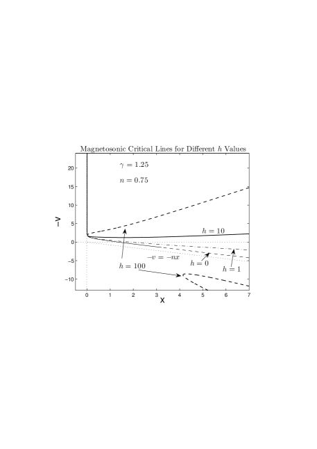
Figure 2: The magnetosonic critical curves for different values of $h$ with given parameters $n=0.75$ and $\gamma=1.25$ ($n=2-\gamma$ for a usual polytropic gas). The light dotted straight line $nx-v=0$ passes through the origin; the two perpendicular light dotted lines represent the abscissa and ordinate axes, respectively. Similar to variation trends shown in Fig. 1, as $h$ increases (i.e., $0,\ 1,\ 10,\ 100$), the average slope $\text{d}(-v)/\text{d}x$ of an individual magnetosonic critical curve increases from negative to positive, and the two segments (i.e., the light solid and dashed lines) for the case of $h=0$ with two different line types correspond to the two sensible roots of equation (34). The magnetosonic critical curve with $h=100$ (heavy dashed lines) has two branches, as indicated in the figure and the lower branch beneath $nx-v=0$.

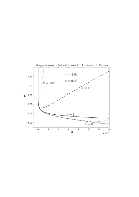
Figure 3: Enlarged version of Fig. 1 with the same parameters yet for much smaller $x$, intended to clearly show the diverging behaviours of the magnetosonic critical curves as $x\rightarrow 0^{+}$. The horizontal $x$ axis is in a numerical scale of $10^{-3}$.

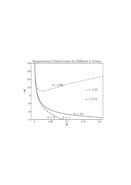
Figure 4: Enlarged version of Figure 2 with the same parameters yet for much smaller $x$, intended to clearly show the diverging behaviours of the magnetosonic critical curves in the limit of $x\rightarrow 0^{+}$.

For a magnetized gas cloud, it is possible to derive another MHD asymptotic series solution in which $v={\cal O}(x)$ and $\alpha\rightarrow+\infty$ as $x\rightarrow 0^{+}$. With the assumption of $v={\cal O}(x)$ and $\alpha^{\gamma}\ll\alpha^{2}x^{2}$ in equation (24), we have $v^{\prime}$ approaching a constant and obtain

$$v=-Cx\ ,$$ (58)

where $C$ is an integration constant. Substituting expression (58) into equations (3.2) and (24), we obtain

$$\alpha^{\prime}=-\frac{\big{[}2h+(n+C)/(3n-2)\big{]}\alpha}{hx}\ ,$$ (59)

$$v^{\prime}=-2(n-1)-\frac{(n+C)^{2}}{h(3n-2)}\ .$$ (60)

By equation (58), this in turn requires

$$2(n-1)+\frac{(n+C)^{2}}{h(3n-2)}=C\$$ (61)

for consistency. Once this quadratic equation (61) for $C$ has at least one positive root of $C$, we obtain at least one possible asymptotic MHD solution in the form of

$$\alpha(x)=Dx^{-2-(n+C)/[(3n-2)h]}\ ,$$ (62)

$$v(x)=-Cx\ ,$$ (63)

where $D$ is yet another integration constant. Quadratic equation (61) for $C$ can be readily solved to give

$$C=-n+\frac{(3n-2)}{2}\left[h\pm(h^{2}-4h)^{1/2}\right]\$$ (64)

and the requirement of $nx-v>0$ is satisfied for both roots of $C$. This immediately requires $h>4$ (i.e., a sufficiently strong magnetic field) for a valid asymptotic MHD solution of this kind. In short, this asymptotic solution for small $x$ is described by

$$v(x)=\bigg{\{}n-\frac{(3n-2)}{2}\left[h\pm(h^{2}-4h)^{1/2}\right]\bigg{\}}x\ ,$$ (65)

$$\alpha(x)=Dx^{-5/2\mp\sqrt{h^{2}-4h}/(2h)}\ ,$$ (66)

$$w(x)=hD^{2}x^{-3\mp\sqrt{h^{2}-4h}/h}\ ,$$ (67)

and the corresponding reduced enclosed mass $m(x)$

$$m(x)=\frac{(3n-2)}{2}D\left[h\pm(h^{2}-4h)^{1/2}\right]x^{1/2\mp\sqrt{h^{2}-4h}/(2h)}\ .$$ (68)

The requirement on $h$ is discussed below. For $\alpha^{\gamma}\ll\alpha^{2}x^{2}$, we obtain the following inequality

$$\gamma<\frac{6h\pm 2(h^{2}-4h)^{1/2}}{5h\pm(h^{2}-4h)^{1/2}}\ .$$ (69)

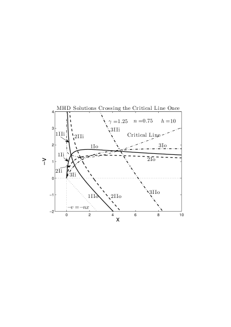
Figure 19: MHD solutions crossing the magnetosonic critical curve once with $\gamma=1.25$, $n=0.75$ and $h=10$. Crossing point 1 corresponds to $\alpha=1$ and $x=0.3998$, crossing point 2 corresponds to $\alpha=0.26$ and $x=1.2053$, and crossing point 3 corresponds to $\alpha=0.12$ and $x=4.6518$, respectively. The two perpendicular light dotted lines are the abscissa and ordinate axes, respectively. The straight line $-v=-nx$ is a demarcation line to the lower left of which solutions become unphysical. The light dash-dotted curve is the magnetosonic critical curve, and the heavy curves are the MHD solutions crossing the magnetosonic critical curve once.

For the upper plus signs, if $\gamma<{6}/{5}$, this requirement is automatically satisfied, while if $\gamma>{6}/{5}$, this requirement means that $h>4/[1-(5\gamma-6)^{2}/(2-\gamma)^{2}]$. For the lower minus signs, if $\gamma<6/5$, this requirement means that $4<h<4/[1-(6-5\gamma)^{2}/(2-\gamma)^{2}]$, while if $\gamma>6/5$, this condition cannot be met, i.e. there does not exist such asymptotic solutions with the lower negative signs. In the absence of magnetic field with $h=0$, this form of asymptotic solution disappears completely. This is a brand-new asymptotic MHD solution in a magnetized gas cloud, and global semi-complete solutions matching this asymptotic solution can be constructed numerically (see Figures 15, 16 and 19 for specific examples). Physically, this asymptotic MHD solution describes a much compressed accreting nucleus where the magnetic pressure $<B_{t}^{2}>/(8\pi)$ becomes much stronger than the thermal gas pressure $p$ to oppose the gravitational collapse such that the reduced radial inflow speed $v(x)$ approaches zero linearly with $x$ as $x\rightarrow 0^{+}$. Physically, we anticipate that a very strong random magnetic field confined to a sufficiently small spatial volume would certainly destroy the quasi-spherical symmetry at some point and drive random flows. We further expect violent and sporadic magnetic activities to destroy the similarity evolution. In spite of all these, we count on the gravity of accreted core materials to more or less control a central sphere. In other words, sufficiently far away from this central magnetized sphere of influence, we may ignore feedbacks of central activities and apply our self-similar MHD inflow solutions. The scenario envisioned here essentially parallels that of a spherical symmetric central inflow without magnetic field. Ultimately, there must be a central object to confront radial inflows and thus destroy the similarity flow evolution. A self-similar flow solution is only valid on large scales and outside a certain sphere surrounding the core. As $x$ approaches zero, the denominators of both equations (3.2) and (24) for this asymptotic series approach $-h\alpha^{2}x^{2}$ and these MHD solutions do not encounter the magnetosonic singular surface. For this asymptotic MHD solution, the magnetic pressure, tension and gravity forces are in the same order of magnitude, all overpowering the thermal gas pressure force, and the magnetic pressure force is the strongest. Including one more term in the series expansion, this novel magnetic asymptotic similarity solution appears as

$$v(x)=\bigg{\{}n-\frac{(3n-2)}{2}\left[h\pm(h^{2}-4h)^{1/2}\right]\bigg{\}}x$$

$$+\gamma D^{\gamma-2}\frac{(3n-2)\big{[}3h-2\pm 3(h^{2}-4h)^{1/2}\big{]}}{(6-5\gamma)h\mp\gamma(h^{2}-4h)^{1/2}}$$

$$\times x^{(2-\gamma)\big{[}5/2\pm\sqrt{h^{2}-4h}/(2h)\big{]}-1}+\cdots\ ,$$ (70)

$$\alpha(x)=Dx^{-5/2\mp\sqrt{h^{2}-4h}/(2h)}+\gamma D^{\gamma-1}$$

$$\times\bigg{[}6h-4\pm 6(h^{2}-4h)^{1/2}+\big{[}5\pm(h^{2}-4h)^{1/2}/h\big{]}$$

$$\times\big{[}(6-5\gamma)h\mp(h^{2}-4h)^{1/2}\big{]}\bigg{]}$$

$$\times\bigg{[}\big{[}(6-5\gamma)h\mp\gamma(h^{2}-4h)^{1/2}\big{]}$$

$$\big{[}(6-5\gamma)h\pm(2-\gamma)(h^{2}-4h)^{1/2}\big{]}\bigg{]}^{-1}$$

$$\times x^{(\gamma-1)\big{[}-5/2\mp\sqrt{h^{2}-4h}/(2h)\big{]}-2}+\cdots\ .$$ (71)

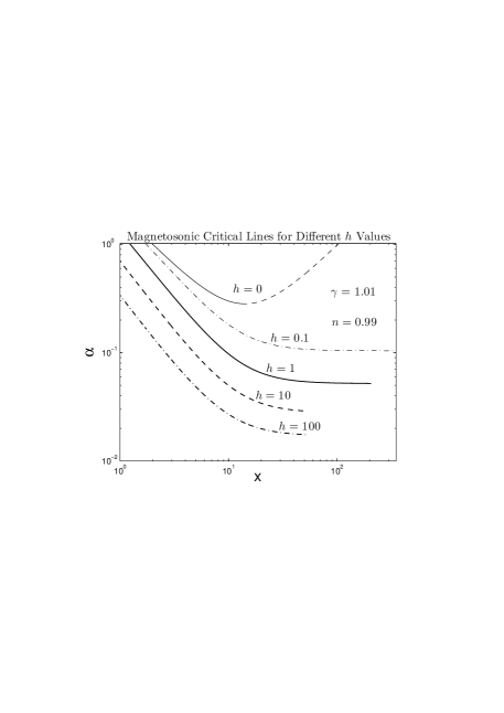
Figure 5: Magnetosonic critical curves of $\alpha$ versus $x$ displayed in logarithmic scales for different values of $h$ with given $\gamma=1.01$ and $n=0.99$ as shown in Figure 1.

3.4.4 A Singular Global Magnetostatic Solution

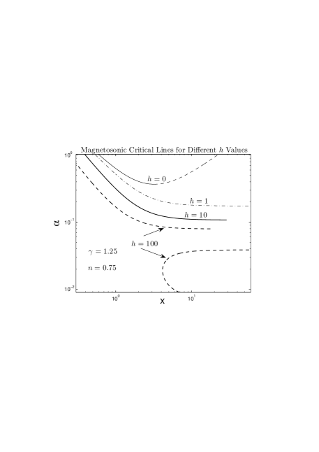
Figure 6: Magnetosonic critical curves of $\alpha$ versus $x$ displayed in logarithmic scales for different values of $h$ with given $\gamma=1.25$ and $n=0.75$ as shown in Figure 2.

For a constant $v$, equation (11) reduces to

$$\quad(nx-v)\alpha^{\prime}=-2\frac{(x-v)}{x}\alpha\ ,$$ (72)

which can be readily integrated for $\alpha(x)$ in the form of

$$\qquad\alpha(x)=cx^{-2}(nx-v)^{2-2/n}\ ,$$ (73)

where $c$ is an integration constant. Along with equation (22), there exists a special singular global magnetostatic solution such that $v=0$ when $n+\gamma=2$, namely

$$v=0\ ,\qquad\alpha=\bigg{[}\frac{(2-\gamma)^{2}}{2\gamma(4-3\gamma)}+\frac{(1-\gamma)}{\gamma}h\bigg{]}^{\frac{1}{\gamma-2}}x^{\frac{-2}{2-\gamma}}\ ,$$

$$m=(2-\gamma)\bigg{[}\frac{(2-\gamma)^{2}}{2\gamma(4-3\gamma)}+\frac{(1-\gamma)}{\gamma}h\bigg{]}^{\frac{1}{\gamma-2}}x^{3-\frac{2}{2-\gamma}}\ .$$ (74)

The reduced magnetic energy density $w(x)$ is

$$w(x)=h\bigg{[}\frac{(2-\gamma)^{2}}{2\gamma(4-3\gamma)}+\frac{(1-\gamma)}{\gamma}h\bigg{]}^{{2}/{(\gamma-2)}}x^{2-{4}/{(2-\gamma)}}\ ,$$ (75)

which diverges as $x\rightarrow 0^{+}$ and vanishes as $x\rightarrow+\infty$. Note that for $h\geq h_{c}$, this global similarity MHD solution does not exist. When $\gamma=2-n$ for a usual polytropic gas, the corresponding ratio of the Alfvén wave speed to the sound speed becomes a constant

$$\frac{v_{A}}{s}=\bigg{(}\frac{h}{\gamma}\bigg{)}^{1/2}\bigg{[}\frac{(2-\gamma)^{2}}{2\gamma(4-3\gamma)}+\frac{(1-\gamma)}{\gamma}h\bigg{]}^{-1/2}\ .$$ (76)

This global similarity MHD solution reduces to that of Suto and Silk (1988) for $h=0$ or $w=0$ as expected. This is a new singular polytropic magnetostatic solution, constructed in the similar manner as has been done before (Shu, 1977; Suto and Silk, 1988; Lou and Shen, 2004). When $h<h_{c}$, this solution encounters the magnetosonic singular surface at the point

$$x= \bigg{[}\frac{2n}{2h+n/(3n-2)}\bigg{]}^{{(\gamma-2)}/{2}}$$ (77)

$$\times\bigg{[}\frac{(2-\gamma)^{2}}{2\gamma(4-3\gamma)}+\frac{(1-\gamma)}{\gamma}h\bigg{]}^{-1/2}\ ,$$

and this point is the intersection of the $v=0$ surface and the magnetosonic critical curve; when $h>h_{c}$, this point does not exist. More precisely, one readily finds that for a fixed $\gamma$, this point moves to infinity as $h$ approaches $h_{c}^{-}$. Expression (77) can also be used to determine the location of the ‘kink point’ of the mEWCSs. In this solution, the four forces, viz. thermal gas pressure, magnetic pressure, magnetic tension and gravity forces are in the same order, and the magnetic pressure force is stronger than the magnetic tension force with a ratio of $-1+2/(2-\gamma)$, with the magnetic pressure gradient force pointing radially outward. In other words, the random magnetic field is not force-free. In the isothermal limit of $\gamma=1$, this ratio becomes unity and the random magnetic field is essentially quasi-force-free (Yu and Lou, 2005; Yu et al., 2006).

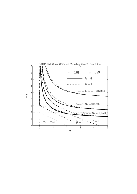
Figure 7: Global numerical similarity MHD solutions in the semi-complete space without crossing the magnetosonic critical curve can be readily constructed using asymptotic solutions (39) and (3.4.1) to start at a sufficiently large $x$ (e.g., $x=100$), with the two parameters $\gamma=1.01$ and $n=0.99$ being specified for a conventional polytropic gas. The two perpendicular dotted lines denote the abscissa and ordinate axes, respectively, and the straight dotted line $-v=-nx$ is the demarcation to the lower left of which solutions become unphysical for a negative enclosed gas mass. The two dash-dotted curves are the sonic ($h=0$) and magnetosonic ($h=1$) critical curves. The solid ($h=0$) and dashed ($h=1$) curves are similarity MHD flow solutions with $h=0$ and $h=1$, respectively; for the first pair solutions with light linetypes, we have both $A_{0}=4$ and $B_{0}=-2$; for the second pair solutions with heavy linetypes, we have both $A_{0}=4$ and $B_{0}=0$; and for the third pair solutions with extremely heavy linetypes, we have both $A_{0}=4$ and $B_{0}=1$ as examples of illustrations for similarity MHD solutions without crossing the critical curves and with outward flow speeds at far-away region.

Note that this solution can also serve as an asymptotic quasi-static condition, with $v$ approaching zero faster than $\sim{\cal O}(x)$ and $\alpha\simeq x^{-2/n}$. These behaviours are primarily caused by the polytropic equation of state with the magnetic field playing the role of modification. This type of asymptotic solutions are referred to as ‘quasi-static’ MHD asymptotic solutions, which can be further sub-divided into two types - type I ‘quasi-static’ MHD asymptotic solutions without oscillations and type II ‘quasi-static’ MHD asymptotic solutions with oscillatory behaviours. A detailed analysis of this asymptotic solution in a polytropic gas without magnetic field has been given by Lou and Wang (2006). We here show such MHD solutions in our figure illustrations (type II ‘quasi-static’ asymptotic solutions in Figures 17 and 18). An analysis of these newly found MHD asymptotic solutions is contained in Appendix G.

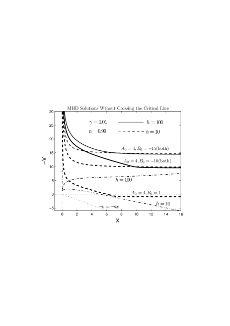
Figure 8: The numerical similarity MHD flow solutions without crossing the magnetosonic critical curve can be readily constructed using asymptotic solutions (39) and (3.4.1) to start at a sufficiently large $x$ (e.g., $x=100$ here), with $\gamma=1.01$ and $n=0.99$ being specified for a conventional polytropic gas. The two perpendicular dotted lines denote the abscissa and ordinate axes, respectively, and the straight dotted line $-v=-nx$ is the demarcation to the lower left of which solutions become unphysical for a negative enclosed gas mass. The two dash-dotted lines are the magnetosonic critical curves for $h=10$ and $h=100$, respectively. The solid and dashed curves are MHD solutions with $h=100$ and $h=10$, respectively; for the pair solutions with light linetypes, we have both $A_{0}=4$ and $B_{0}=-15$, while for the other pair solutions with heavy linetypes, we have both $A_{0}=4$ and $B_{0}=-10$. The dashed curve with $A_{0}=4$ and $B_{0}=1$ for $h=10$ (with an extremely heavy linetype) is an example of MHD similarity solutions without crossing the magnetosonic critical curve and with an outward flow speed in the far-away region.

3.4.5 A Global MHD Expansion Solution

For a constant $\alpha$ in equation (11), we obtain

$$v^{\prime}={2(x-v)}/{x}\ ,$$ (78)

which can be readily integrated to attain

$$v={2}x/{3}+cx^{2}\ ,$$ (79)

where $c$ is an integration constant. By equation (22), we should set $c=0$ and thus obtain a global MHD solution

$$v=\frac{2x}{3}\ ,\ \ \ \alpha=\frac{2}{3(6h+1)}\ ,\ \ \ m=\frac{2(n-2/3)}{3(6h+1)}x^{3}$$ (80)

accordingly; the reduced magnetic energy density $w$ is

$$w(x)=\frac{4hx^{2}}{9(6h+1)^{2}}\ ,$$ (81)

which increases with $x$ quadratically along with the increase of the radial flow speed $v$ linearly in $x$. For a polytropic gas with $\gamma=2-n$, the ratio of the Alfvén wave speed to the sound speed becomes

$$\frac{v_{A}}{s}=\bigg{(}\frac{h}{\gamma}\bigg{)}^{1/2}\left[\frac{2}{3(6h+1)}\right]^{(2-\gamma)/2}x\ .$$ (82)

This solution reaches the singular surface at

$$x=\bigg{[}\frac{\gamma(4/3)^{\gamma}/(18h+3)^{\gamma}}{2(n-2/3)^{2}/(18h+3)-4h/(18h+3)^{2}}\bigg{]}^{1/2}$$

on the magnetosonic critical curve.

3.4.6 Asymptotic MHD Expansion
   Solutions in the Limit of Large $x$

Solutions (80) and (81) can also be regarded as an asymptotic solution as $x$ approaches infinity. To leading orders, the asymptotic MHD solution can be written as

$$v(x)=\frac{2}{3}x+v_{0}\ ,$$

$$\alpha=\frac{2}{3(6h+1)}\qquad$$

$$-\frac{9(3n+1)(3n-2)(6h+1)^{2}-6(6h+1)}{6(n-3/2)^{2}(3n-2)(6h+1)-2h(3n-2)}\frac{v_{0}}{x}\ ,\qquad$$ (83)

where $v_{0}$ is an integration constant. In this case, the denominators of both equations (3.2) and (24) approach

$$\frac{2}{3(6h+1)}\bigg{[}\bigg{(}n-\frac{2}{3}\bigg{)}^{2}-\frac{2h}{3(6h+1)}\bigg{]}x^{2}$$

which does not encounter the magnetosonic critical curve, unless under extremely rare situations.

3.4.7 Regular Similarity MHD Solutions for Small $x$

We may assume an asymptotic MHD series solution as

$$\alpha(x)=\alpha_{\ast}+\alpha_{1}x+\alpha_{2}x^{2}+\cdots,$$

$$v(x)=v_{0}+v_{1}x+v_{2}x^{2}+\cdots\ ,$$ (84)

as $x$ approaches zero. Substitution of solution (84) into equations (11) and (22) leads to

$$v(x)=\frac{2}{3}x-\frac{\alpha_{\ast}^{(1-\gamma)}}{15\gamma}\bigg{[}(6h+1)\alpha_{\ast}-\frac{2}{3}\bigg{]}\bigg{(}n-\frac{2}{3}\bigg{)}x^{3}+\cdots\ ,$$ (85)

$$\alpha(x)=\alpha_{\ast}-\frac{\alpha_{\ast}^{(2-\gamma)}}{6\gamma}\bigg{[}(6h+1)\alpha_{\ast}-\frac{2}{3}\bigg{]}x^{2}+\cdots\ ,$$ (86)

$$w(x)=h\alpha_{\ast}^{2}x^{2}-2h\frac{\alpha_{\ast}^{(2-\gamma)}}{6\gamma}\bigg{[}(6h+1)\alpha_{\ast}-\frac{2}{3}\bigg{]}x^{4}+\cdots\ .$$ (87)

For a usual polytropic gas with $\gamma=2-n$ and for very small $x$, the corresponding ratio of the Alfvén wave speed $v_{A}$ to the sound speed $s$ becomes

$${v_{A}}/{s}=(h\alpha_{\ast}^{2-\gamma}/\gamma)^{1/2}x\ ,$$ (88)

which vanishes as $x\rightarrow 0^{+}$. As $x$ approaches zero, the denominators of both equations (3.2) and (24) for this series expansion approach $-\gamma\alpha^{\gamma}$ and these solutions do not encounter the magnetosonic singular surface. For this asymptotic solution, the four forces including the thermal pressure, magnetic pressure, magnetic tension and gravity forces are in the same order, and the magnetic pressure and tension forces tend to be the same in magnitude. The magnetic pressure gradient force points radially outward.

3.5 Asymptotic Behaviours of Critical Curves

Asymptotic behaviours of magnetosonic critical curves are important from a global perspective. We summarize below the major asymptotic behaviours of critical curves with or without magnetic field, respectively.

Case I for $h\neq 0$ in the presence of magnetic field.

(i) The limiting regime of $\alpha\rightarrow+\infty$. According to quadratic equation (34), the asymptotic quadratic equation of $x^{2}$ for the magnetosonic critical curve is

$$\frac{h\alpha^{3}}{(3n-2)^{2}}x^{4}+\frac{\gamma\alpha^{\gamma+1}}{(3n-2)^{2}}x^{2}-4\gamma^{2}\alpha^{2\gamma-2}=0\ ,$$ (89)

which has only one positive root of small $x$

$$x^{2}\cong 4(3n-2)^{2}\alpha^{\gamma-3}\ ,$$ (90)

and along with equation (33), one obtains correspondingly a diverging radial inflow speed

$$v\cong-\sqrt{\gamma}\alpha^{(\gamma-1)/2}\ .$$ (91)

As $\alpha$ approaches positive infinity, $x$ approaches zero and $v$ approaches $-\infty$. This appears to be the case also for a purely hydrodynamic case with $h=0$ (Lou and Wang, 2006) and was not discussed in Suto and Silk (1988). Thus, the magnetosonic critical curve does not intersect the $v-$axis as compared to the isothermal unmagnetized cases (Shu, 1977; Lou and Shen, 2004) where the sonic critical line is the straight line $-v=1-x$. For a magnetized isothermal gas (Yu and Lou, 2005; Yu et al., 2006), the magnetosonic critical lines are curves intersecting the $v-$axis.

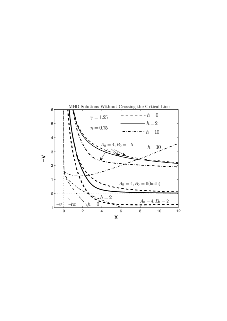
Figure 9: Similarity MHD flow solutions without crossing the magnetosonic critical curve with the values of $\gamma=1.25$ and $n=0.75$ being specified for a usual polytropic gas. The perpendicular dotted lines denote the abscissa and ordinate axes, respectively, and the straight dotted line $-v=-nx$ is a demarcation to the lower left of which the solutions become unphysical for a negative enclosed mass. The light dash-dotted curves are the magnetosonic critical curves for $h=0,\ 2,\ 10$. The dashed and solid curves are global solutions with $h=0$ and $h=2$, respectively (heavy linetypes: $A_{0}=4$ and $B_{0}=0$; light linetypes: $A_{0}=4$ and $B_{0}=-5$). The heavy dash-dotted curve is the solution with $h=10$, $A_{0}=4$ and $B_{0}=-5$. The dashed curve with $A_{0}=4$ and $B_{0}=2$ for $h=0$ (the extremely heavy linetype) is an example of hydrodynamic similarity solutions without crossing the sonic critical curve and with an outward flow speed in the far-away region.

(ii) The limiting case of $x\rightarrow+\infty$. According to equation (33), we obtain the following condition for $\alpha$

$$\pm\bigg{[}n-1+\frac{\alpha}{(3n-2)}\bigg{]}(h\alpha)^{1/2}=-n(n-1)\ ,$$ (92)

and correspondingly, the behaviour of $v$ versus $x$ as

$$v\cong[n\mp(h\alpha)^{1/2}]x\ .$$ (93)

This means that as $x$ approaches infinity, $v$ varies linearly with $x$ and $\alpha$ approaches a certain constant value determined by equation (92). This linear behaviour of $v$ in $x$ is qualitatively similar to the isothermal case (Shu, 1977; Lou and Shen, 2004), where the sonic critical line is a straight line throughout the entire semi-complete space; we note that for the isothermal and non-magnetized case, $\alpha$ approaches zero as the sonic critical line approaches infinity. For a magnetized gas cloud, the slope of this linear relation now depends on $h$ parameter. By the constraint of $m(x)>0$, the lower signs in solutions (92) and (93) are unphysical, yet mathematically these equations may describe asymptotic behaviours of a new branch of critical line.

The special case of $h=h_{c}$ with $h_{c}$ defined by equation (44) should be noted with interest. In this case, the corresponding value of $\alpha$ as $x\rightarrow+\infty$ becomes

$$\alpha=2(1-n)(3n-2)\ ,$$ (94)

giving rise to $(h\alpha)^{1/2}=n$ and thus the vanishing of the leading order term of $v$ by the upper minus sign in equation (93). This hints that the magnetosonic critical curve tends to be parallel to the $x-$axis as $x$ approaches infinity. Naturally for $(h\alpha)^{1/2}>n$ as $x\rightarrow+\infty$, one infers that $h>h_{c}$ and vice versa. This reveals an interesting trend of variation that as $h$ exceeds the critical value $h_{c}$, the magnetosonic critical curve will head up (i.e., increase eventually) towards the first quadrant (see subsection 4.1) and $h=h_{c}$ marks the marginal case for the asymptotic behaviour of the magnetosonic critical curve at large $x$.

Case II for $h=0$ in the absence of magnetic field.

As $\alpha\rightarrow+\infty$, the asymptotic quadratic equation for $x^{2}$ now becomes

$$n^{2}(n-1)^{2}x^{4}-\frac{\gamma\alpha^{\gamma+1}x^{2}}{(3n-2)^{2}}+4\gamma^{2}\alpha^{2\gamma-2}=0\ ,$$ (95)

[see equation (89) in parallel for the different coefficient of the first term $x^{4}$] which has two positive roots for $x^{2}$.

(i) For the small $x$ regime of

$$x^{2}\cong 4\gamma(3n-2)^{2}\alpha^{\gamma-3}\ ,$$ (96)

one obtains a diverging radial inflow speed of

$$v\cong-\sqrt{\gamma}\alpha^{(\gamma-1)/2}\ .$$ (97)

As $x$ approaches zero, $\alpha$ approaches positive infinity while $v$ approaches negative infinity. Again, the sonic critical curve does not intersect the $v-$axis in contrast to the isothermal case (Shu, 1977; Lou and Shen, 2004). Compared with the isothermal case, this sonic critical curve behaviour appears to be a unique feature for a polytropic gas (Lou and Wang, 2006, 2007), not realized before (Suto and Silk, 1988). For an isothermal magnetized cloud (Yu and Lou, 2005; Yu et al., 2006), the magnetosonic critical curve involves a cubic equation in terms of $v$; the physical portion of the curve still intersects the $v-$axis (see figures 1 and 2 of Yu and Lou, 2005).

(ii) For the large $x$ regime of

$$x^{2}\cong\frac{\gamma\alpha^{\gamma+1}}{n^{2}(n-1)^{2}(3n-2)^{2}}\$$ (98)

and accordingly

$$v\cong nx\ ,$$ (99)

we have the variation trend for the magnetosonic critical curve such that as $x$ approaches infinity, $\alpha$ approaches infinity and $v$ increases with $x$ linearly. This feature differs from the isothermal case (Shu, 1977; Lou and Shen, 2004); in the isothermal case with $n=1$, the above asymptotic behaviour is invalid although the asymptotic behaviour (99) seems valid.

3.6 Series Expansions near the
      Magnetosonic Critical Curve

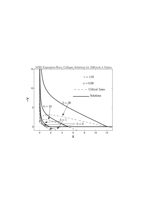
Figure 10: Examples of semi-complete MHD expansion wave collapse solutions (mEWCSs) and the corresponding magnetosonic critical curves for different $h$ values with $B_{0}=0$, $\gamma=1.01$ and $n=0.99$ being specified for a usual polytropic gas. The two perpendicular dotted straight lines are the abscissa and ordinate axes, respectively, and the dash-dotted curves are the magnetosonic critical curves. The heavy solid curves are the mEWCSs. The corresponding values of $A_{0}$ for the cases of $h=0$, $1$, $10$ and $30$ are $2.0133$, $2.0544$, $2.5163$ and $5.004$, respectively.

Generally, smooth analytical solutions cannot go across the singular surface as noted in Section 3.3 unless they cross the magnetosonic critical curve. Along the magnetosonic critical curve, one cannot calculate the derivatives of the variables directly from nonlinear MHD ODEs (3.2) and (24). From equation (11), we use

$$\alpha^{\prime}=\frac{\alpha v^{\prime}-2\alpha(x-v)/x}{(nx-v)}\$$ (100)

to compute $\alpha^{\prime}$ once $v^{\prime}$ is known. Applying the L’H$\hat{\mbox{o}}$pital rule to equation (3.2), we immediately obtain the following quadratic equation in terms of $v^{\prime}$

$$A_{2}(v^{\prime})^{2}+B_{2}v^{\prime}+C_{2}=0\$$ (101)

along the magnetosonic critical curve, where the three coefficients $A_{2}$, $B_{2}$ and $C_{2}$ are defined explicitly by

$$A_{2}\equiv 1+\frac{(\gamma^{2}\alpha^{\gamma-1}+2h\alpha x^{2})}{(\gamma\alpha^{\gamma-1}+h\alpha x^{2})}\ ,$$

$$B_{2}\equiv n+1-4\frac{(\gamma^{2}\alpha^{\gamma-1}+2h\alpha x^{2})}{(\gamma\alpha^{\gamma-1}+h\alpha x^{2})}$$

$$+4\bigg{[}\frac{(\gamma^{2}\alpha^{\gamma-1}+2h\alpha x^{2})}{(\gamma\alpha^{\gamma-1}+h\alpha x^{2})}-1\bigg{]}\frac{v}{x}+\frac{4h\alpha x}{(nx-v)}\ ,$$

$$C_{2}\equiv 2\bigg{[}\frac{2(\gamma^{2}\alpha^{\gamma-1}+2h\alpha x^{2})}{(\gamma\alpha^{\gamma-1}+h\alpha x^{2})}-1\bigg{]}\frac{v^{2}}{x^{2}}$$

$$+2\bigg{[}\frac{\alpha}{(3n-2)}-2n-4\frac{(\gamma^{2}\alpha^{\gamma-1}+2h\alpha x^{2})}{(\gamma\alpha^{\gamma-1}+h\alpha x^{2})}+4\bigg{]}\frac{v}{x}$$

$$+\frac{(n-2)\alpha}{(3n-2)}+2\bigg{[}n+2\frac{(\gamma^{2}\alpha^{\gamma-1}+2h\alpha x^{2})}{(\gamma\alpha^{\gamma-1}+h\alpha x^{2})}-2\bigg{]}$$

$$+2h\alpha\bigg{[}1-\frac{4(x-v)}{(nx-v)}\bigg{]}\ .$$ (102)

By setting $h=0$, equations (101) and (3.6) reduce to the hydrodynamic results (Suto and Silk, 1988) as a necessary requirement; by further letting $\gamma\rightarrow 1$, these two equations reduce to those of the isothermal case (Shu, 1977). For $h\neq 0$ and letting $\gamma\rightarrow 1$, these two equations are equivalent to those of the isothermal MHD case (Yu and Lou, 2005; Yu et al., 2006). One can determine eigensolution behaviours by Taylor series expansions near the magnetosonic critical curve using equations (101) and (3.6). By quadratic equation (101), one obtains two types of eigensolutions across the magnetosonic critical curve.

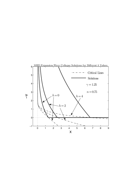
Figure 11: Examples of semi-complete mEWCSs and the corresponding magnetosonic critical curves for different $h$ values with $B_{0}=0$, $\gamma=1.25$ and $n=0.75$ being specified for a usual polytropic gas. The two perpendicular dotted straight lines are the abscissa and ordinate axes, respectively, and the dash-dotted curves are the magnetosonic critical curves. The heavy solid curves represent mEWCSs. The corresponding values of $A_{0}$ parameter for the cases of $h=0$, $2$ and $4$ are $1.151$, $2.520$ and $21.55$, respectively.

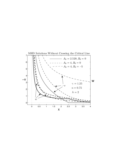
Figure 12: Examples of semi-complete similarity MHD flow solutions without crossing the magnetosonic critical curve. The reduced magnetic energy density $w$ associated with a random transverse magnetic field is displayed in curves (right ordinate) using heavy linetypes and the corresponding $-v$ is in curves (left ordinate) using light linetypes. The $-v$ curves are the same as those in Figure 9. The case of $A_{0}=2.520$ and $B_{0}=0$ (solid curve) is an mEWCS, while the case of $A_{0}=4$ and $B_{0}=0$ (dashed curve; not an mEWCS) is a global similarity MHD flow.

For the unmagnetized isothermal case, Whitworth and Summers (1985) noticed that there are different behaviours near the vicinity of the sonic critical line, depending on the topological structure of paths through a sonic point. This topological structure is investigated by the eigenvalues of the following matrix

$$\left(\begin{matrix}A_{\alpha}&A_{v}&A_{x}\cr V_{\alpha}&V_{v}&V_{x}\cr X_{\alpha}&X_{v}&X_{x}\cr\end{matrix}\right)$$ (103)

where $A$, $V$ and $X$ are the three functions defined by equations (3.2), (3.2) and (27), respectively, and $A_{\alpha}$ denotes a partial differentiation of $A$ with respect to $\alpha$, taking $\alpha$, $v$ and $x$ as three independent variables; other symbols follow the same notational convention by inference. The explicit expressions of the partial differentiations contained in the above matrix are summarized in Appendix B. The characteristic equation for the matrix (103) is simply

$$\left|\begin{matrix}\lambda-A_{\alpha}&-A_{v}&-A_{x}\cr-V_{\alpha}&\lambda-V_{v}&-V_{x}\cr-X_{\alpha}&-X_{v}&\lambda-X_{x}\cr\end{matrix}\right|=0\ ,$$ (104)

and the signs of the $\lambda$ roots determine the behaviours in the vicinity of the magnetosonic critical curve. Equation (104) is equivalent to

$$\lambda^{3}-\big{(}A_{\alpha}+V_{v}+X_{x}\big{)}\lambda^{2}+\big{(}A_{\alpha}V_{v}+A_{\alpha}X_{x}+V_{v}X_{x}$$

$$-A_{x}X_{\alpha}-A_{v}V_{\alpha}-X_{v}V_{x}\big{)}\lambda-X_{\alpha}A_{v}V_{x}-A_{\alpha}V_{v}X_{x}$$

$$+X_{\alpha}V_{v}A_{x}+X_{x}V_{\alpha}A_{v}+A_{\alpha}V_{x}X_{v}-V_{\alpha}A_{x}X_{v}=0\ ,$$

which can be cast into a succinct form of

$$\lambda^{3}+B_{3}\lambda^{2}+C_{3}\lambda+D_{3}=0\ ,$$ (106)

with apparent definitions for the three coefficients $B_{3}$, $C_{3}$ and $D_{3}$ by referring to equation (3.6). Because the magnetosonic critical curve is continuous, this characteristic equation must have one zero root, i.e., $D_{3}=0$, corresponding to a path which stays on the magnetosonic curve (see Whitworth and Summers 1985 for a reference and Appendix D for a proof). The other two eigenvalues for $\lambda$ of matrix (103) are then given by quadratic equation

$$\lambda^{2}+B_{3}\lambda+C_{3}=0\ .$$ (107)

The behaviours in the vicinity of the magnetosonic critical curve depend upon the signs of the two $\lambda$ roots of quadratic equation (107).

Case I. For a negative determinant $B_{3}^{2}-4C_{3}<0$, we have a spiral or a centre case (e.g., Jordan and Smith, 1977). In this case, the solutions do not have a one-to-one correspondence to $x$ and are thus regarded as unphysical. For a polytropic magnetized gas, such points may exist (see Appendix F).

Case II. For a positive determinant $B_{3}^{2}-4C_{3}>0$ with $C_{3}<0$, we have a saddle point along the magnetosonic critical curve with two eigensolutions determined by equations (100), (101) and (3.6). Numerical integrations away from these saddle points tend to be stable.

Case III. For a positive determinant $B_{3}^{2}-4C_{3}>0$ with $C_{3}>0$, we have a nodal point along the magnetosonic critical curve with infinitely many solutions crossing the magnetosonic critical curve. As noted by Hunter (1986), among these solutions only the two eigensolutions are analytical, while others involve weak discontinuities or weak shocks (e.g., Boily and Lynden-Bell, 1995) and might be unstable (e.g., Lazarus, 1981). Although only integrations towards nodal points are stable, to pick out the analytic eigensolutions among the solutions having weak discontinuities, we have integrated outward from these points using second-order derivatives. Explicit expressions of the relevant second-order derivatives are summarized in Appendix C.

Case IV. For a vanishing determinant $B_{3}^{2}-4C_{3}=0$, we have inflection nodal points. If $C_{3}=0$, we have degenerate points along the magnetosonic critical curve.

4 Global Similarity Solutions

Table 1: The corresponding $m(0)$ values for similarity MHD flow solutions without crossing the magnetosonic critical curve for a polytropic gas with $\gamma=1.01$ and $n=0.99$ and relatively small values of $h$ parameter. The two coefficients $A_{0}$ and $B_{0}$ are specified in asymptotic MHD solutions (39) and (3.4.1). Parameter $m(0)$ is directly computed from equation (10). Here, the $m(0)$ value is computed after integrating from large $x$ values such as $x=100$ to small $x$ values.

$h$	$0$	$0$	$1$	$1$
$A_{0}$, $B_{0}$	$4,\ 0$	$4,\ -2$	$4,\ 0$	$4,\ -2$
$m(0)$	$5.513$	$12.34$	$5.912$	$12.48$

Table 2: The corresponding $m(0)$ values for similarity MHD solutions without crossing the magnetosonic critical curve for a polytropic gas with $\gamma=1.01$ and $n=0.99$ and relatively large values of $h$ parameter. The two coefficients $A_{0}$ and $B_{0}$ are specified in asymptotic MHD solutions (39) and (3.4.1). Parameter $m(0)$ is directly computed from equation (10). Here, the $m(0)$ value is computed after numerically integrating from large $x$ values such as $x=100$ to small $x$ values.

$h$	$10$	$10$	$100$	$100$
$A_{0}$, $B_{0}$	$4,\ -10$	$4,\ -15$	$4,\ -10$	$4,\ -15$
$m(0)$	$40.28$	$57.59$	$44.58$	$59.09$

With compatible initial and boundary conditions together with a proper treatment of the magnetosonic critical curve, the two coupled nonlinear MHD ODEs for self-similar collapses and flows can be integrated numerically. We have explored MHD solutions numerically, including the properties of the magnetosonic critical curve and $\alpha-v-x$ solutions of the MHD ODEs. In Suto and Silk (1988), both cases of $n=1$ and $n=2-\gamma$ were considered; here, we focus on the case of a usual polytropic gas with $n=2-\gamma$. In contrast to the case of $\gamma<1$ considered by Fatuzzo et al. (2004), we are mainly concerned with the range of $1<\gamma<4/3$. We intend to find semi-complete solutions valid in the range of $0<x<+\infty$, and discuss how such MHD solutions can be constructed through numerical integrations.

4.1 Magnetosonic Critical Curves

The magnetosonic critical curves for different parameters can be systematically searched by numerical means, and for the completion of a magnetosonic critical curve, one needs the relevant analytical results summarized in subsections 3.3 and 3.5. We have extensively explored the behaviours of magnetosonic critical curves for specified values of $n$, $\gamma$ and $h$ parameters, and present the main results below. More details can be found in Appendix E.

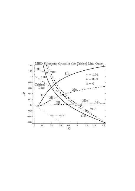
Figure 13: Hydrodynamic polytropic solutions crossing the sonic critical curve once, with $\gamma=1.01$, $n=0.99$ and $h=0$. Point 1 corresponds to $\alpha=5$ and $x=0.3941$, point 2 corresponds to $\alpha=3$ and $x=0.6570$, and point 3 corresponds to $\alpha=2$ and $x=0.9877$, respectively. The two perpendicular light dotted straight lines are abscissa and ordinate axes, respectively, while the light dotted straight line passing through the origin is $-v=-nx$ to the lower left of which solutions become unphysical for a negative enclosed mass. The light dash-dotted line is the sonic critical curve, and the heavy lines are the solutions crossing the sonic critical curve once.

First, we show magnetosonic critical curves with different values of $h$ for given $n=0.99$ and $\gamma=1.01$ (Figs. 1 and 3). A magnetosonic critical curve may be divided into two parts as one picks up different roots of quadratic equation (34) for $x^{2}$.

When $h$ increases for stronger magnetic field strengths, the average slope $\text{d}(-v)/\text{d}x$ of an individual magnetosonic critical line increases from negative to positive in our figure displays of $-v$ versus $x$. Meanwhile as the magnetic field becomes strong enough and as $x$ approaches infinity, $v$ may approach $-\infty$. The critical value $h_{c}$ in this specific case is $50.521$ (see subsection 3.5). This feature is important in the numerical analysis of similarity MHD flow solutions not crossing the magnetosonic critical curve. In contrast to the straight sonic critical line for the isothermal unmagnetized case (Shu, 1977; Lou and Shen, 2004), the magnetosonic critical curves here diverge as $x$ approaches zero (see Fig. 3).

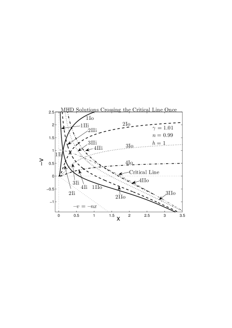
Figure 14: Similarity MHD solutions crossing the magnetosonic critical curve once, with $\gamma=1.01$, $n=0.99$ and $h=1$ being specified for a conventional polytropic gas. Point 1 corresponds to $\alpha=15$ and $x=0.1200$, point 2 corresponds to $\alpha=5$ and $x=0.3214$, point 3 corresponds to $\alpha=2$ and $x=0.7021$, and point 4 corresponds to $\alpha=1$ and $x=1.2456$, respectively. The two perpendicular light dotted straight lines are abscissa and ordinate axes, respectively, while the light dotted straight line passing through the origin is $-v=-nx$ to the lower left of which solutions become unphysical for a negative enclosed mass. The light dash-dotted line is the magnetosonic critical curve, and the heavy lines are the solutions crossing the magnetosonic critical curve once.

The magnetosonic critical curves in this nearly isothermal case of $\gamma\geq 1$ can be compared with those of the isothermal MHD case of $\gamma=1$ (Yu and Lou, 2005; Yu et al., 2006). Their asymptotic behaviours are different for both limiting regimes of $x\rightarrow 0^{+}$ and $x\rightarrow+\infty$. As $x$ approaches zero, the magnetosonic critical curve in the isothermal case intersects with the vertical $v-$axis, while in the nearly isothermal MHD case it diverges as $x\rightarrow 0^{+}$. As $x$ approaches infinity, the magnetosonic critical curve in the isothermal case remains in the fourth quadrant, while in the nearly isothermal case it can head up to the first quadrant. These qualitative differences in asymptotic behaviours in such parallel cases result from equations $(\ref{wang45})-(\ref{wang47})$. According to equation (91), for $\gamma=1$, $v$ remains finite as $x$ approaches zero, while for $\gamma\geq 1$, even a small increment in $\gamma$ will lead to a divergence of $v$ as $x$ goes to zero. In accordance with equation (92), if $n=1$ as in the isothermal case, $\alpha$ must approach zero as $x$ approaching infinity, which means that $v\sim nx$, i.e. the magnetosonic critical curve remains in the fourth quadrant. Nonetheless when $n$ is not equal to unity, this constraint on asymptotic behaviour of the magnetosonic critical curve disappears. Another perspective is that when $n\rightarrow 1$, we have $h_{c}\rightarrow\infty$; thus whatever $h$ values will lead to asymptotic behaviours such that $v\rightarrow+\infty$ as $x\rightarrow+\infty$.

The magnetosonic critical curves for different values of $h$ given $n=0.75$ and $\gamma=1.25$ are shown in Fig. 2. When $h$ increases, again the average slope $\text{d}(-v)/\text{d}x$ of an individual magnetosonic critical line increases from negative to positive in the $-v$ versus $x$ presentation. The value of $h_{c}$ is $4.5$ in this example. As the magnetic field becomes extremely strong, one obtains another branch of the magnetosonic critical curve as shown in Fig. 2 for $h=100$. This new branch is the one mentioned in equation (33). The lower branch of the heavy dotted curve is unphysical for being to the lower left of the straight line $-v=-nx$. Also the magnetosonic critical curve diverges as $x$ approaches zero.

Table 3: The corresponding $m(0)$ values for self-similar MHD flow solutions without crossing the magnetosonic critical curve for a conventional polytropic gas of $\gamma=1.25$ and $n=0.75$ with different values of $h$. The two parameters $A_{0}$ and $B_{0}$ are specified in asymptotic MHD solutions (39) and (3.4.1). Parameter $m(0)$ is directly computed from equation (10). Here, the $m(0)$ value is computed after integrating from large $x$ values such as $x=100$ to small $x$ values.

$h$	$0$	$0$	$2$	$2$	$10$
$A_{0}$, $B_{0}$	$4,\ 0$	$4,\ -5$	$4,\ 0$	$4,\ -5$	$4,\ -5$
$m(0)$	$3.8185$	$4.952$	$3.664$	$4.919$	$4.747$

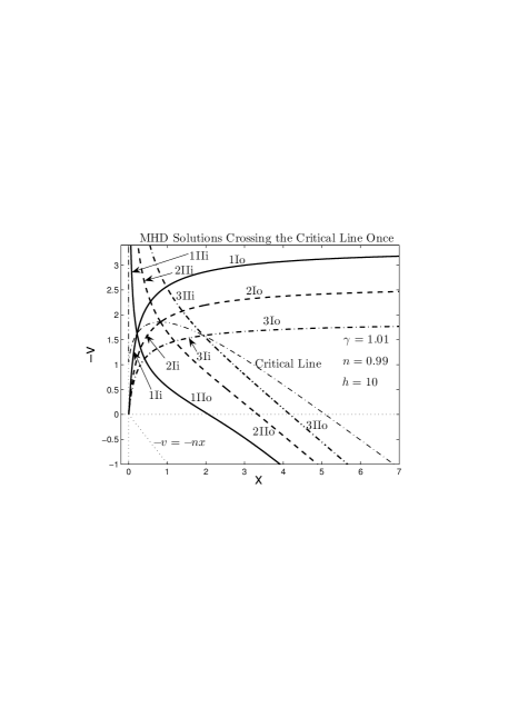
(a) The smaller $x$ regime. Crossing points 1, 2, and 3 correspond to $\alpha=5$ and $x=0.2170$, $\alpha=0.9$ and $x=0.8255$, and $\alpha=0.3$ and $x=1.9389$, respectively.

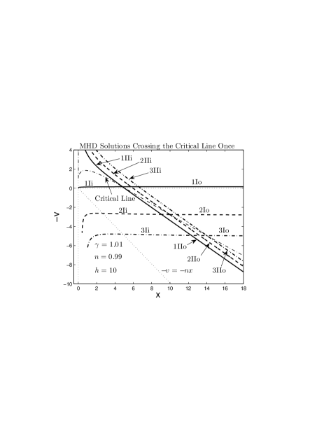
(b) The larger $x$ regime. Crossing points 1, 2, and 3 correspond to $\alpha=0.1$ and $x=4.8147$, $\alpha=0.05$ and $x=9.9587$, and $\alpha=0.04$ and $x=14.0005$, respectively.

Figure 15: MHD solutions crossing the magnetosonic critical curve once, with $\gamma=1.01$, $n=0.99$ and $h=10$. Panel (a) displays the solutions crossing the magnetosonic critical curve at smaller $x$, while panel (b) displays those crossing the magnetosonic critical curve at larger $x$. The two perpendicular light dotted lines are abscissa and ordinate axes, respectively, and the light dotted straight line is for $-v=-nx$. The light dash-dotted line is the magnetosonic critical curve, and the heavy curves are the MHD solutions crossing the magnetosonic critical curve once.

Table 4: For Figure 10, we summarize the corresponding $m(0)$ values and the $x$ values of the ‘kink point’ $x_{k}$ for MHD expansion wave collapse solutions for $\gamma=1.01$ and $n=0.99$ for a conventional polytropic gas (see Yu & Lou 2005 and Yu et al. 2006 for an isothermal magnetized gas).

$h$	$0$	$1$	$10$	$30$
$m(0)$	$1.0120$	$1.4931$	$4.346$	$19.26$
$x_{k}$	$1.019$	$1.76$	$5.08$	$12.11$

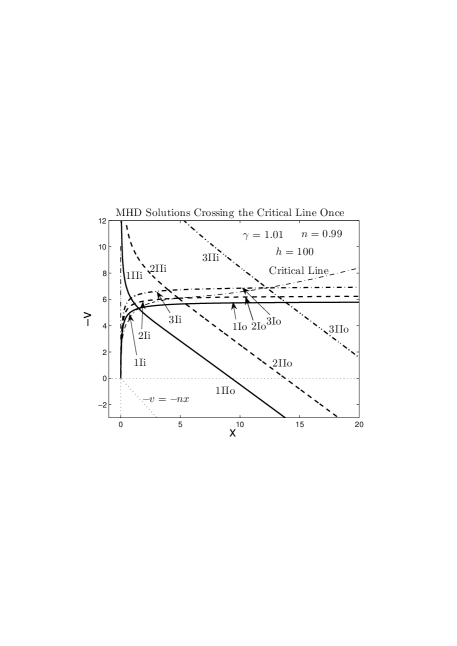
Figure 16: MHD solutions crossing the magnetosonic critical curve once with parameters $\gamma=1.01$, $n=0.99$ and $h=100$ being specified. Crossing point 1 corresponds to $\alpha=0.2$ and $x=1.5055$, point 2 corresponds to $\alpha=0.05$ and $x=4.8487$, and point 3 corresponds to $\alpha=0.024$ and $x=12.2494$, respectively. The two perpendicular light dotted straight lines are abscissa and ordinate axes, respectively, and the light dotted straight line is the demarcation line $-v=-nx$. The light dash-dotted line is the magnetosonic critical curve, and the heavy curves are the solutions crossing the magnetosonic critical curve once.

Table 5: For Figure 11, we summarize the corresponding $m(0)$ and the $x$ values of the ‘kink point’ values $x_{k}$ for MHD expansion wave collapse solutions with two parameters $\gamma=1.25$ and $n=0.75$ specified for a usual polytropic gas (see Yu and Lou 2005 for an isothermal magnetized gas).

$h$	$0$	$2$	$4$
$m(0)$	$0.7992$	$2.083$	$24.38$
$x_{k}$	$1.37$	$2.52$	$6.68$

Enlarged features for diverging behaviours of $v(x)$ along the magnetosonic critical curves for small $x$ in Figs. 1 and 2 are shown in Figs. 3 and 4, respectively. The corresponding features of $\alpha$ versus $x$ are displayed in Figs. 5 and 6, respectively. The basic facts that for $h=0$, $\alpha$ approaches infinity both as $x$ approaches zero and infinity, while for $h>0$, $\alpha$ approaches infinity as $x$ approaches zero and $\alpha$ approaches a constant as $x$ goes to infinity are all consistent with the relevant analytical results presented in subsection 3.5.

By numerical exploration, we found that the magnetosonic critical curve has two branches in the $\gamma=1.01$, $n=0.99$ case with $h=1000$. Also, the critical curve consists of two parts as shown in Fig. 1 in the case of $h=0$ can also be found in the case of $\gamma=1.01$, $n=0.99$, and $h=0.03$. From the results for critical curves, one can see that asymptotic analyses in subsections 3.3 and 3.5 are necessary for determining the entire magnetosonic critical curve.

4.2 Solutions without crossing the Magnetosonic Critical Curve and MHD Expansion Wave Collapse Solutions

4.2.1 General MHD Solutions without Crossing the Magnetosonic Critical Curve

Among the asymptotic MHD solutions derived in subsection 3.4, the series expansion at large $x$ described by equations (39) and (3.4.1) can be readily integrated from large values of $x$ inward to obtain numerical solutions without encountering the magnetosonic critical curve. Specifically, we integrate the solutions from a starting point of $x=100$.

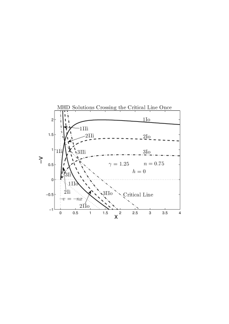
Figure 17: Hydrodynamic solutions crossing the sonic critical curve once, with $\gamma=1.25$, $n=0.75$ and $h=0$. Crossing point 1 corresponds to $\alpha=5$, $x=0.1386$, crossing point 2 corresponds to $\alpha=2$ and $x=0.3166$, and crossing point 3 corresponds to $\alpha=1$ and $x=0.6131$, respectively. The two perpendicular light dotted lines are the abscissa and ordinate axes, respectively, and the light dotted straight line $-v=-nx$ is the demarcation line to the lower left of which solutions become unphysical. The light dash-dotted line is the sonic critical curve, and the heavy curves are the solutions crossing the sonic critical curve once. The oscillatory behaviours of solutions 1Ii, 2Ii and 3Ii as $x$ approaches $0$ are not readily seen and will be discussed at the end of the main text.

We present such global semi-complete similarity MHD solutions for the case of $\gamma=1.01$ and $n=0.99$ in both Figures 7 and 8. Note that when $x$ approaches zero, the solution approaches the free-fall state as discussed in subsection 3.4 [see equations (50) and (51)]. Note also that the major difference in $v(x)$ of the two solutions with the same values of $A_{0}$ and $B_{0}$ but with different magnetic field strengths (i.e., different $h$) manifests mainly at small $x$ about $0\leq x\leq 10$ in both Figures. Both Figs. 7 and 8 show that the magnetic field mainly accelerates the central collapses, i.e. when $h$ is larger, the $-v(x)$ becomes larger at the same $x$, although the asymptotic behaviours of $v(x)$ as $x$ approaches infinity show that larger $h$ implies smaller $-v(x)$ at the same large $x$.

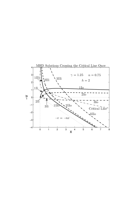
Figure 18: MHD solutions crossing the magnetosonic critical curve once with $\gamma=1.25$, $n=0.75$ and $h=2$ being specified. Crossing point 1 corresponds to $\alpha=1$ and $x=0.5107$, crossing point 2 corresponds to $\alpha=0.4$ and $x=1.1549$, and crossing point 3 corresponds to $\alpha=0.18$ and $x=3.7395$, respectively. The two perpendicular light dotted lines are the abscissa and ordinate axes, respectively, and the light dotted straight line $-v=-nx$ is the demarcation to the lower left of which solutions become unphysical. The light dash-dotted curve is the magnetosonic critical curve, and the heavy curves are the solutions crossing the magnetosonic critical curve once. The oscillatory behaviours of solutions 1Ii, 2Ii and 3Ii as $x$ approaches $0$ are not readily seen and will be discussed at the end of the main text.

Numerical similarity MHD solutions for the case of $\gamma=1.25$ and $n=0.75$ are presented in Figure 9. In this figure the solution with the same values of $A_{0}$ and $B_{0}$ but larger $h$ value cannot catch up with the other solutions with smaller values of $h$. This does not necessarily mean that the net magnetic force does not accelerate collapses, because of a smaller $-v$ in the initial state for the case of a larger $h$.

We briefly note several points here. Firstly, we analyzed in subsection 3.4 the asymptotic behaviour of the MHD free-fall solutions for small $x$ and inferred from that analysis that these solutions will not encounter the magnetosonic singular surface at small $x$, meanwhile the asymptotic MHD solutions as $x$ approaches infinity [equations (39) and (3.4.1)] also do not encounter the singular surface. Therefore, these numerical MHD solutions are specific examples of semi-complete solutions without crossing the magnetosonic critical curve or encountering the singular surface. Secondly, there exists a two-dimensional continuum regime of parameters $A_{0}$ and $B_{0}$ for this series expansion of MHD solution, e.g., for a specified $A_{0}$ parameter, parameter $B_{0}$ should be larger than a certain threshold value in order to construct MHD similarity flow solutions without encountering the magnetosonic critical curve. Outside such allowed parameter regime, the solutions tend to crash on to the singular surface but away from the magnetosonic critical curve so that a global semi-complete MHD solution does not exist. Thirdly, the MHD similarity flow solutions with $h>h_{c}$ will cross the magnetosonic critical curve at the projection to $-v\sim x$ plane, yet they do not actually cross the magnetosonic critical curve in the $\alpha-v-x$ space because they do not encounter the singular surface.

4.2.2 Construction of MHD Expansion
   Wave Collapse Solutions (mEWCSs)

One interesting solution among global MHD solutions not crossing the magnetosonic critical curve is the limiting solution corresponding to MHD expansion wave collapse solutions (mEWCSs) as a generalization of the isothermal EWCS (Shu, 1977) in two important aspects, i.e., the polytropic gas and the inclusion of a random magnetic field. We emphasize here the existence of such global MHD similarity solutions because magnetic fields do exist in molecular clouds in general and play important roles in the evolution of a collapsing cloud. From the perspectives of dynamic evolution, diffusive processes, radiative signatures, formations of discs and jets and origin of stellar magnetic fields, one must take into account of magnetic fields in molecular clouds. By the model scenario here, our analysis suggests that there exist mEWCSs for $h<h_{c}$ (a weaker magnetic field), while no such mEWCS exists for $h\geq h_{c}$ (a stronger magnetic field).

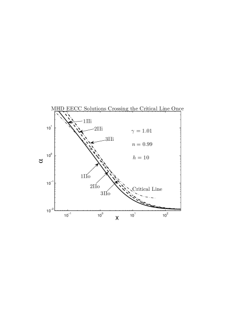
Figure 20: Corresponding $\alpha$ behaviours for the MHD solutions 1II, 2II and 3II in Fig. 15(a). The light dash-dotted curve is the magnetosonic critical curve, and the heavy curves are the solutions crossing the magnetosonic critical curve once.

This conclusion can be viewed from the following perspectives. First, in asymptotic MHD solutions (39) and (3.4.1), parameter $B_{0}$ can be regarded as an external (or initial) radial flow speed more or less independent of the mass density profile. For example in the isothermal case, parameter $B_{0}$ represents an asymptotic steady flow speed in regions far from the core (see Lou and Shen 2004 and subsection 3.4 here). Parameter $A_{0}$ contributes to the radial speed profile due to gas mass density distribution and the associated self-gravity. To construct mEWCSs, one should require that $B_{0}=0$ and the reduced radial speed $v(x)$ approaches $0^{-}$, i.e., for the limiting series solution, the radial flow velocity remains negative and approaches zero far away. In this limiting regime, a magnetized gas cloud of quasi-spherical symmetry remains at rest in early times and the core collapse is induced by self-gravity. In this perspective, the critical $A_{0}$ for mEWCS is determined by setting the coefficient of $x^{(n-2)/n}$ term [from the same two terms $x^{{(n-2)}/{n}}$ and $x^{(2-2\gamma-n)/n}$ for a usual polytropic gas with $n=2-\gamma$] in asymptotic MHD solution (3.4.1) to vanish. In contrast, the case of $h\geq h_{c}$ corresponds to positive coefficients of both terms involving $A_{0}$ in asymptotic MHD solution (3.4.1) because of ${1}/{(3n-2)}+{2h(n-1)}/{n^{2}}<0$, indicating outward expansions for any value of $A_{0}>0$ when the coefficient of $x^{(n-2)/n}$ term vanishes. Secondly, for a mEWCS, the reduced velocity remains zero at large $x$ until the solution meets the magnetosonic critical curve at the point where the magnetosonic critical curve intersects the $x-$axis. At this intersection point, the slope of the magnetosonic critical curve is negative for $h<h_{c}$, which allows the mEWCS to head up as $x\rightarrow 0^{+}$, while for $h\geq h_{c}$, the slope of the magnetosonic critical curve is positive to force the solution to crash on to the singular surface without leading to a mEWCS. Thirdly, the physical reason for the non-existence of a mEWCS when $h>h_{c}$ is that a sufficiently strong magnetic field tends to prevent a gravitational collapse and to drive an outward expansion instead. The stability analysis of the present MHD problem remains to be examined for the case of $h\geq h_{c}$. For $h\geq h_{c}$ a magnetized gas cloud collapses only when external (initial) inflows are present. Because of $h_{c}\rightarrow\infty$ in the isothermal case, any $h$ may lead to an mEWCS. Finally, when $h\geq h_{c}$ or $A_{0}$ smaller than a certain critical value representing the mEWCS, parameter $B_{0}$ should be negative to ensure the core collapse of a magnetized gas cloud. When $B_{0}$ becomes sufficiently negative, the corresponding initial flow speed profile will have a tendency to collapse, and a core collapse without encountering the magnetosonic critical curve can happen. Therefore for any $A_{0}>0$, one can find solutions without encountering the magnetosonic critical curve.

In Figures 10 and 11, we present the mEWCSs of a usual polytropic gas cloud for $\gamma=1.01$, $n=0.99$ and $\gamma=1.25$, $n=0.75$, respectively. We conclude from both Figures 10 and 11 that the kink points $x_{k}$ of the mEWCSs have larger $x$ values as $h$ increases. The corresponding values of $m(0)$ and $x_{k}$ are summarized in Tables 4 and 5, respectively.

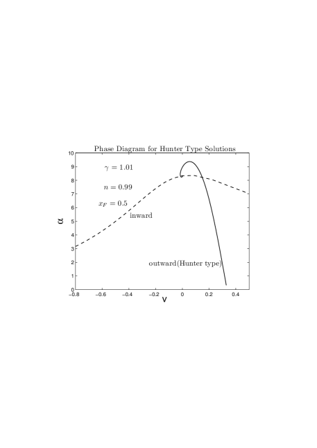
Figure 21: Density-speed phase diagram for MHD generalizations of Hunter type solutions with $\gamma=1.01$, $n=0.99$, $h=1$, and a chosen meeting point at $x_{F}=0.5$. The ‘outward’ curve represents the phase path of Hunter type solutions when the parameter $\alpha_{\ast}$ is changed gradually. The ‘inward’ curve represents the phase path of solutions crossing the magnetosonic critical curve as the intersection point of the MHD solutions with the magnetosonic critical curve is gradually adjusted.

We also present the reduced magnetic energy density $w=h\alpha^{2}x^{2}$ associated with a random transverse magnetic field ${\mathbf{B}}_{t}$ versus $x$. Figure 12 collects a sample of $w$ versus $x$ solution curves for $\gamma=1.25$, $n=0.75$ and $h=2$ (see Fig. 9). Note that the initial magnetic field strengths are the same $hA_{0}^{2}x^{(2-4/n)}$ as $x$ approaches infinity (i.e., $t\rightarrow 0^{+}$) for the two upper curves (i.e., dashed and dash-dotted linetypes) with $A_{0}=4$; at first the magnetic field strength increases faster in the case of $B_{0}=0$ as $x$ becomes smaller, and then at some point around $x=0.63549$ the curve with larger initial velocity ($B_{0}=-5$) catches up with the former and grows faster. For the mEWCS with $A_{0}=2.520$ and $B_{0}=0$ and a decreasing $x$, the reduced magnetic energy density $w$ begins to increase before the kink point $x_{k}=2.6$ in the reduced velocity field, and at the kink point the magnetic field also appears to increase more slowly than at larger $x$ values. The interpretation of this feature is that at a specific point, the magnetic field first maintains a constant and then begins to decrease when the magnetosonic wave front reaches this point.

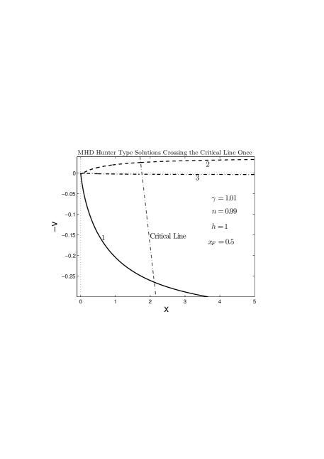
Figure 22: The first three discrete MHD Hunter type solutions for $\gamma=1.01$, $n=0.99$, $h=1$ and $x_{F}=0.5$ in the semi-complete space. The two perpendicular light dotted lines are the abscissa and ordinate axes. The light dash-dotted curve is the magnetosonic critical curve and the heavy lines are the similarity MHD solutions curves. Curve 1 corresponds to $\alpha_{\ast}=359.37$ and crosses the magnetosonic critical curve at $x=2.1154$, curve 2 corresponds to $\alpha_{\ast}=8.3941\times 10^{6}$ and crosses the magnetosonic critical curve at $x=1.7248$, and curve 3 corresponds to $\alpha_{\ast}=1.4769\times 10^{11}$ and crosses the magnetosonic critical curve at $x=1.7637$, respectively. As $x\rightarrow+\infty$, the two corresponding $A_{0}$ and $B_{0}$ in asymptotic solutions (39) and (3.4.1) are $A_{0}=2.430$ and $B_{0}=0.3810$ for curve 1, $A_{0}=2.016$ and $B_{0}=-0.03998$ for curve 2, and $A_{0}=2.058$ and $B_{0}=0.003869$ for curve 3, respectively.

Table 6: Values of the two parameters $A_{0}$ and $B_{0}$ in equations (39) and (3.4.1) at large $x$ of relevant semi-complete similarity MHD flow solutions in Figures 13 through 19.

Parameters $A_{0}$ and $B_{0}$ in equations (39) and (3.4.1)
Fig.	15(a)	15(a)	15(a)	15(b)	16
Curve	1Io	2Io	3Io	1Io	1Io
$A_{0}$	0.145	0.535	1.110	2.392	0.448
$B_{0}$	-3.468	-2.704	-1.934	-0.166	-6.074
Fig.	16	16	19	19	19
curve	2Io	3Io	1Io	2Io	3Io
$A_{0}$	1.222	3.812	0.268	0.767	9.447
$B_{0}$	-6.556	-7.340	-3.268	-2.948	-5.204

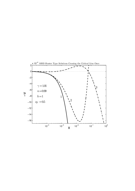
Figure 23: Enlarged versions for the MHD generalizations of the first three Hunter type MHD solutions for $\gamma=1.01$, $n=0.99$, $h=1$ and $x_{F}=0.5$ to illustrate that the $i$th solution has $i$ stagnation points ($i=1,\ 2,\ 3$). Other parameters are the same as those in Figure 22. Note that the ordinate scale has a factor of $10^{-4}$ and the abscissa for $x$ is in the logarithmic scale. The feature of self-similar magnetosonic oscillations is shown by these MHD solutions, as a general extension of the isothermal hydrodynamic feature revealed by Hunter 1977 and Lou & Shen 2004.

Table 7: Corresponding $m(0)$ values of MHD free-fall solutions at small $x$ for relevant semi-complete solutions in Figs. 13 through 19.

Corresponding values of $m(0)$ for MHD free-fall solutions
Fig.	15(a)	15(a)	15(a)	15(b)	15(b)	15(b)
Curve	1IIi	2IIi	3IIi	1IIi	2IIi	3IIi
$m(0)$	0.400	1.291	2.442	4.213	6.933	10.18
Fig.	16	16	16	19	19	19
Curve	1IIi	2IIi	3IIi	1IIi	2IIi	3IIi
$m(0)$	2.539	8.345	35.59	0.260	0.741	11.44

One readily obtains the corresponding value of $m(0)$ for each MHD free-fall solution using equation (10). The corresponding $m(0)$ values for all solutions computed in this section are summarized in Tables 1 to 5. According to Tables 1 and 2, one finds that $m(0)$ increases with either larger $h$ or larger magnitude of $B_{0}$, indicating that a stronger magnetic field and a faster inward initial speed both result in a more rapid core collapse and lead to an enhanced central mass accretion (n.b. profiles of gas mass density scalings remain the same). This is related to the fact that the inward magnetic tension force is twice as large as the outward magnetic pressure gradient force. In reference to Table 4, we note the increase of $m(0)$ with a larger $h$ in mEWCSs with the two parameters $\gamma$ and $n$ being specified. By Table 3, one finds that a larger $B_{0}$ results in a smaller $m(0)$, but as mentioned above this does not necessarily mean that the magnetic field does not accelerate the core collapse because of an initial smaller velocity. By Table 5, one again gets an increase of $m(0)$ with increasing $h$. We also provide the $x$ values of the corresponding ‘kink points’ $x_{k}$ of the mEWCSs in Tables 4 and 5, showing that for a given $\gamma>1$, the corresponding $x_{k}$ increases with an increasing $h$ value as long as $h<h_{c}$.

4.3 Numerical MHD Solutions Crossing the Magnetosonic Critical Curve Once

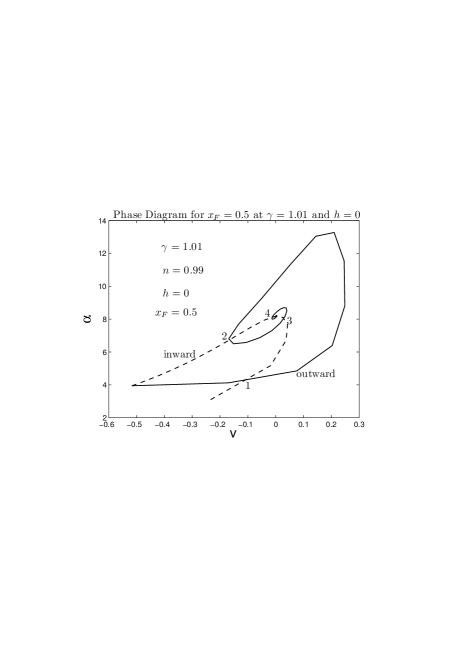
Figure 24: Density-speed phase diagram of $\alpha$ versus $v$ for $\gamma=1.01$, $n=0.99$, $h=0$ and $x_{F}=0.5$. The ‘inward curve’ (dashed curve) denotes the phase path by integrating inward from different $x$ ($x>x_{F}$) along the sonic critical curve to reach $x_{F}$, using the type I eigensolution, while the ‘outward curve’ denotes the phase path integrating from different $x$ ($x<x_{F}$) along the sonic critical curve to reach $x_{F}$, using the type II eigensolution. The spiral pattern of the outward curve suggests the trend of infinitely many matches, leading to infinitely many semi-complete polytropic EECC solutions (see Lou and Shen 2004).

Behaviours of similarity MHD flow solutions around the magnetosonic critical curve are determined by equations $(\ref{wang53})-(\ref{wang55})$, where the first derivatives of $v(x)$ and $\alpha(x)$ with respect to $x$ can be determined along the magnetosonic critical curve. Numerically, one can integrate from a point in the vicinity of the magnetosonic critical curve away to obtain a portion of the eigensolution crossing the magnetosonic critical curve. At one specific point on the magnetosonic critical curve, there exist two eigensolutions crossing the magnetosonic critical line. The one of smaller $v^{\prime}$ in the vicinity of the magnetosonic critical line is denoted as type I solutions and the other of larger $v^{\prime}$ is type II solutions [for a sufficiently small $x$, these parallel with type 1 and type 2 derivatives, respectively (Lou and Shen, 2004)]. These notations differ from those used in the isothermal case (Shu, 1977; Lou and Shen, 2004). We have explored MHD solutions crossing the magnetosonic critical curve once, with several typical results shown in Figs. 13 to 19. For mnemonics, we denote the type Y (Y=I, II) solution outward (inward) from the $x$th ($x=1,\ 2,\ 3,\ 4$) point by $x$Yo ($x$Yi) solution. We searched similarity MHD solutions for the cases of $\gamma=1.01$, $n=0.99$ and of $\gamma=1.25$, $n=0.75$ with various $h$ values, i.e., different reduced magnetic energy density. We mainly focus on semi-complete physical solutions in $0^{+}<x<+\infty$.

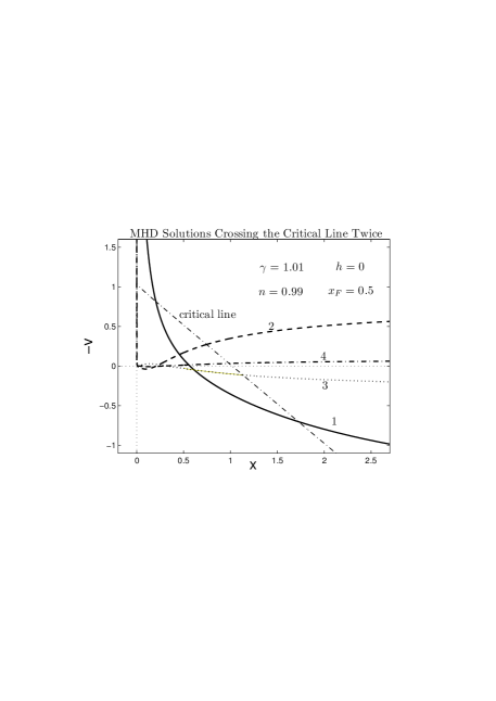
Figure 25: Corresponding to the matches in the density-speed phase diagram of Figure 24, the first four hydrodynamic polytropic solutions with $\gamma=1.01$, $n=0.99$, $h=0$ and $x_{F}=0.5$ are shown here. Curve 1 (solid line) is obtained from $x=1.7248$ ($\alpha=1.15739$, $v=0.7018$) and $x=0.2035$ ($\alpha=9.7036$, $v=-0.8150$) along the sonic critical curve (this is a type I$-$type II match), curve 2 (dashed line) is obtained from $x=0.7448$ ($\alpha=2.64742$, $v=-0.2726$) and $x=2.2124\times 10^{-4}$ ($\alpha=9224.0$, $v=-1.0517$) along the sonic critical curve, curve 3 (dotted line) is obtained from $x=1.1319$ ($\alpha=1.74780$, $v=0.1128$) and $x=4.9114\times 10^{-6}$ ($\alpha=4.2354\times 10^{5}$, $v=-1.0722$) along the sonic critical curve, and curve 4 (dash-dotted line) is obtained from $x=0.9855$ ($\alpha=2.00440$, $v=-0.0329$) and $x=2.8282\times 10^{-8}$ ($\alpha=7.5482\times 10^{7}$, $v=-1.1004$) along the sonic critical curve.

4.3.1 Solutions with $\gamma=1.01$ and Small $h$ Values

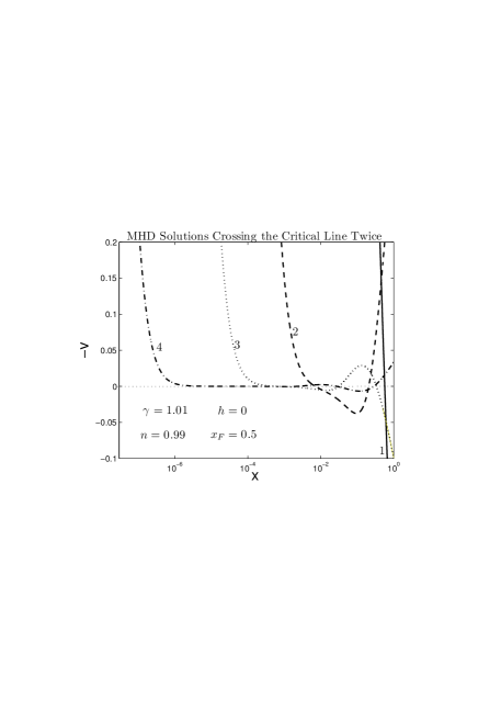
Figure 26: Corresponding to Figs. 24 and 25, the enlarged versions of the first four solutions for smaller $x$ in a logarithmic scale with $\gamma=1.01$, $n=0.99$, $h=0$ and $x_{F}=0.5$ are shown with stagnation points and radial oscillations. Curves 1, 2, 3 and 4 are the same as those in Fig. 25.

Figure 27: Density-speed phase diagram for specified parameters $\gamma=1.01$, $n=0.99$, $h=1$ and a chosen meeting point $x_{F}=0.5$. The ‘inward curve’ is the phase path obtained by integrating inward from different $x$ ($x>x_{F}$) along the magnetosonic critical curve to reach $x_{F}$, using the type I MHD eigensolution, while the ‘outward curve’ denotes the phase path integrating from different $x$ ($x<x_{F}$) along the magnetosonic critical curve to reach $x_{F}$, using the type II MHD eigensolution. The spiral pattern of the ‘outward curve’ hints at infinitely many matches, leading to infinitely many semi-complete MHD EECC similarity solutions.

Figure 28: Corresponding to the three meeting point matches in the phase diagram of Figure 27, we show the first three MHD similarity solutions with $\gamma=1.01$, $n=0.99$, $h=1$ and $x_{F}=0.5$. Curve 1 (solid line) is obtained from $x=2.1065$ ($\alpha=0.526485$, $v=0.2580$) and $x=0.001157$ ($\alpha=1747.8$, $v=-1.0432$) along the magnetosonic critical curve, curve 2 (dashed line) is obtained from $x=1.7248$ ($\alpha=0.671990$, $v=-0.02598$) and $x=5.5880\times 10^{-8}$ ($\alpha=3.8072\times 10^{7}$, $v=-1.0966$) along the magnetosonic critical curve, and curve 3 (dash-dotted line) is obtained from $x=1.7637$ ($\alpha=0.653929$, $v=0.002533$) and $x=3.3391\times 10^{-12}$ ($\alpha=6.6905\times 10^{11}$, $v=-1.1516$) along the magnetosonic critical curve, respectively. For the convenience of visual inspection, we have multiplied curve 3 by a factor of 5, i.e., $-5v$ is shown here for curve 3.

Hydrodynamic solutions with $\gamma=1.01$, $n=0.99$ and $h=0$ are shown in Figure 13. Solutions 1Ii, 2Ii and 3Ii for small $x$ values all run under the straight demarcation line $-v=-nx$ (to the lower left of which solutions become unphysical) and then encounter the singular surface (without crossing the sonic critical curve); they are thus not valid at small $x$ neither mathematically nor physically. Solutions 1IIo, 2IIo and 3IIo crash on to the singular surface and are invalid at large $x$ mathematically, although one may expect special solutions crossing the critical line twice at some specific points in a discrete manner (see subsection 4.4 and Lou and Shen 2004. Solutions 1IIi, 2IIi and 3IIi approach the free-fall solution [equations (50) and (51)] and are valid for small $x$. Solutions 1Io, 2Io and 3Io approach asymptotic solutions (39) and (3.4.1) and are also valid at large $x$. Solutions shown in Fig. 13 fail to form semi-complete hydrodynamic polytropic solutions. Likewise, MHD solutions with the same $\gamma$ and $n$ but $h=1$ shown in Fig. 14 also fail to form semi-complete MHD solutions, and the validity of each MHD solution is just like the corresponding one in Fig. 13, i.e., MHD solutions 1Ii, 2Ii and 3Ii run to the lower left of the demarcation line $-v=-nx$ and then crash on to the singular surface, solutions 1IIo, 2IIo and 3IIo crash on to the singular surface, solutions 1IIi, 2IIi and 3IIi approach the MHD free-fall solution and solutions 1Io, 2Io and 3Io approach asymptotic MHD solutions (39) and (3.4.1).

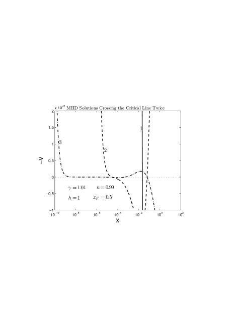
Figure 29: The enlarged version of the first three MHD EECC solutions with $\gamma=1.01$, $n=0.99$, $h=1$ and $x_{F}=0.5$ in a logarithmic scale for small $x$ to show the stagnation points with $v=0$ and self-similar magnetosonic radial oscillations. Curves 1, 2 and 3 are the same as those in Figure 28.

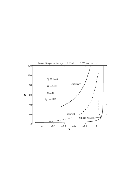
Figure 30: Density-speed phase diagram for $\gamma=1.25$, $n=0.75$, $h=0$ and $x_{F}=0.2$. The ‘inward curve’ is the phase curve obtained by integrating inward from different $x$ ($x>x_{F}$) along the sonic critical curve to reach the chosen $x_{F}$ using the type I eigensolution, and the ‘outward curve’ denotes the phase path integrating from different $x$ ($x<x_{F}$) along the sonic critical curve to reach $x_{F}$ using the type II eigensolution. There is no spiral pattern for the ‘outward curve’ and only one single match can be found at the lower-right corner.

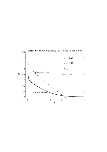
Figure 31: Corresponding to the single match in the density-speed phase diagram of Figure 30, the relevant hydrodynamic polytropic solution $-v(x)$ versus $x$ (solid curve) is shown here for $\gamma=1.25$, $n=0.75$, $h=0$ and $x_{F}=0.2$, with the two crossing points given by $x=3.1529$ ($\alpha=0.36876104$, $v=1.3777$) and $x=0.01197$ ($\alpha=80.978$, $v=-1.9275$) along the sonic critical curve (dash-dotted curve).

4.3.2 Solutions with $\gamma=1.01$ and Larger $h$ Values

For a larger $h$ value of stronger magnetic field, we show a few more examples of semi-complete MHD flow solutions. Fig. 15 shows the solutions with $\gamma=1.01$, $n=0.99$ and $h=10$. The solutions 1Ii, 2Ii, 3Ii in Fig. 15(a) and 1Ii in Fig. 15(b) approach asymptotic MHD solutions (62) and (63) with $C=7.62$ which is the same for all four solutions here. Solutions 1Io, 2Io and 3Io in both panels (a) and (b) approach the asymptotic forms of (39) and (3.4.1) at large $x$, with the corresponding parameters $A_{0}$ and $B_{0}$ summarized in Table 6. Solutions 1IIi, 2IIi and 3IIi in both panels (a) and (b) approach the MHD free-fall solution at smaller $x$ with $m(0)$ summarized in Table 7. Solutions 1IIo, 2IIo and 3IIo in both panels (a) and (b) approach asymptotic MHD solution (3.4.6). Solutions 2Ii and 3Ii in Fig. 15(b) run to the lower left of the demarcation line $-v=-nx$ and then crash on to the singular surface (not crossing the magnetosonic critical curve) and are thus invalid in the small $x$ regime. Therefore in Fig. 15, among the twelve solution branches (I1, I2, I3, II1, II2 and II3 in both panels), there exist in total ten semi-complete solutions, all but the two solution branches 2I and 3I in Fig. 15(b). In Fig. 16, the solutions are also all semi-complete solutions and the corresponding parameters are tabulated in Tables 6 and 7. The corresponding $C$ parameter in equations (62) and (63) for this case is $C=95.0$. The novel asymptotic MHD solutions (62) and (63) have been used here and the relevant numerical MHD results are consistent with the analytical analysis.

4.3.3 Solutions with $\gamma=1.25$ and Small $h$ Values

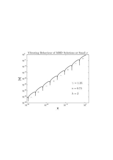
Figure 36: An example for the magnetosonic oscillation behaviour of an MHD similarity solution at small $x$ with both $|v|$ (the absolute value of $v$) and $x$ displayed in logarithmic scales. Relevant parameters are $\gamma=1.25$, $n=0.75$ and $h=2$. This similarity MHD solution is obtained by integrating from the point $\alpha=0.18$, $x=3.7395$ and $v=0.3863$ on the magnetosonic critical curve inward to $x=0$. The alternating plus and minus signs marked along the curve denote the actual sign of $-v$ to compensate the loss of sign information as we show $|v|$ in a logarithmic scale here. The plot clearly suggests that the velocity amplitude scales with $x$ in a power law.

For a usual polytropic gas with a different combination of larger $\gamma$ and smaller $n$, e.g., $\gamma=1.25$ and $n=0.75$, the situation remains qualitatively similar, but in the smaller $x$ regime with also a small $h$, the situation appears somewhat different. Fig. 17 presents the unmagnetized case of $h=0$ where solutions 1Ii, 2Ii and 3Ii show self-similar oscillation behaviours about the $x$ axis for the regime of small $x$ (see Fig. 36 and the isothermal case Lou & Shen 2004). This MHD oscillation behaviour, however, differs from that described by Lou and Shen (2004), mainly because it is of type II ‘quasi static’ (i.e., the infall speed remains finite) asymptotic solution as was recently discovered in the hydrodynamic case (Lou and Wang, 2006); the presence of such ‘quasi-static’ asymptotic solutions is intimately related to the polytropic equation of state. Given other parameters the same but for $h=2$, Fig. 18 displays semi-complete MHD solutions 1II, 2II and 3II, with the inner portions approaching the MHD free-fall state with parameter $m(0)$ summarized in Table 7 and the outer portions approaching asymptotic MHD solutions (3.4.6). Meanwhile, MHD solutions 1Ii, 2Ii and 3Ii clearly display the self-similar magnetosonic oscillation behaviours for smaller $x$ in an analogous manner. This confirms the existence of the ‘quasi-static’ asymptotic behaviour in our MHD model. An analysis of such MHD solutions is contained in Appendix G.

4.3.4 MHD Solutions with $\gamma=1.25$ and Larger $h$ Values

For an even larger $h$ such as $h=10$, one can construct semi-complete MHD solutions for both types. Besides the similar type of 1II, 2II and 3II solutions with parameter $m(0)$ also contained in Table 7, MHD solutions 1I, 2I and 3I are also valid both in small and large $x$ regimes. The corresponding $C$ in solutions (62) and (63) for MHD solutions 1Ii, 2Ii and 3Ii is $C=1.47$, and the parameters $A_{0}$ and $B_{0}$ of equations (39) and (3.4.1) are summarized in Table 6. The self-similar magnetosonic oscillation behaviour is described in section 5. The novel asymptotic MHD solutions also exist for $\gamma=1.25$.

4.3.5 Solution Behaviours of $\alpha$ versus $x$

Behaviours of the corresponding $\alpha(x)$ solution profile of the MHD EECC solutions in Fig. 15(a) are presented in Fig. 20. Note that the $\alpha(x)$ profiles of all three MHD solutions approach the same limiting constant $2/[3(6h+1)]$ at large $x$ as expected. Other MHD EECC solutions in the figures above are similar to these solutions. This type of solutions represents a magnetized gas in spherical envelope expansion with a constant reduced density $\alpha$ at large $x$ (initially) and a free-falling core for small $x$ (finally). For a specified set of $\gamma$, $n$ and $h$, this series of MHD solutions may form a one-dimensional continuum, depending on the point where they cross the magnetosonic critical curve. In other words, by adjusting the crossing point where such kind of MHD solutions intersect the magnetosonic critical curve, we are able to construct infinitely many such solutions and thus the collection of this kind of MHD solutions forms a one-dimensional continuum. We emphasize that this series solutions constructed are closely related to the random magnetic field in the problem. Complementary to the hydrodynamic EECC solutions (Lou and Shen, 2004), the new MHD EECC solutions in this subsection have different asymptotic behaviours at large $x$. The fact that solution (80) also serves as an asymptotic behaviour at large $x$ [see equation (3.4.6)] should be emphasized here; we further confirm the validity of this asymptotic MHD solution by calculating one more term in the series expansion of this asymptotic MHD solution.

4.3.6 MHD Hunter Type Solutions

Another type of MHD solutions crossing the magnetosonic critical curve once is here referred to as the Hunter type solution (Hunter, 1977) generalized to a magnetized polytropic gas and parallel to isothermal examples shown in figure 6 of Lou and Shen (2004). We obtain these MHD series solutions by solution matching in the phase diagram at a chosen meeting point $x=x_{F}$ where these two solutions have the same values of $\alpha$, $v$, $\alpha^{\prime}$ and $v^{\prime}$. In reference to EECC solutions in the isothermal and unmagnetized formulation (Lou and Shen, 2004), we expect that for $\gamma$ close to unity and $h$ not very large, MHD generalizations of this Hunter type of solutions should exist. We explored the case of $\gamma=1.01$, $n=0.99$ and $h=1$, and chose a meeting point at $x_{F}=0.5$. The matching in the phase diagram is displayed in Figure 21 with a familiar spiral pattern, indicating that there may exist infinitely many matches, corresponding to infinitely many discrete semi-complete MHD solutions of this type. Figure 22 presents the first three such MHD solutions and Figure 23 is an enlarged version of Figure 22 revealing that the number of stagnation points increases for these solutions. These features show self-similar magnetosonic oscillations in a magnetized polytropic gas. These similarity solutions are the MHD counterparts of the isothermal hydrodynamic solutions (Hunter, 1977; Lou and Shen, 2004).

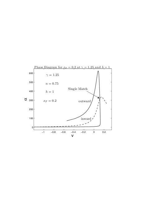
Figure 32: Density-speed phase diagram for $\gamma=1.25$, $n=0.75$, $h=1$ and a chosen meeting point $x_{F}=0.2$. The ‘inward curve’ is the phase path by integrating inward from different $x$ ($x>x_{F}$) along the magnetosonic critical curve to reach a chosen $x_{F}=0.2$ using the type I MHD eigensolution, and the ‘outward curve’ denotes the phase path integrating from different $x$ ($x<x_{F}$) along the magnetosonic critical curve to reach $x_{F}$ using the type II MHD eigensolution. There is no spiral pattern for the ‘outward curve’ and only one single match exists.

4.4 Similarity Solutions Crossing the Magnetosonic Critical Curve Twice

There exist semi-complete MHD solutions crossing the magnetosonic critical curve twice. We explore them using the procedure of Lou and Shen (2004). The advantage of being able to reduce from three coupled nonlinear MHD ODEs to two will become apparent as we manage to match solutions in a two-dimensional phase space of $v(x)$ and $\alpha(x)$.

We chose different meeting points, denoted by $x_{F}$, in the cases of $\gamma=1.01$ and $\gamma=1.25$, for a usual polytropic gas with $n=2-\gamma$. In general, higher values of $h$ do not lead to matches in the range $0.01-0.8$ for $x_{F}$ values that we have systematically searched. For $\gamma=1.01$ and smaller $h$ or $h=0$, we find that there are likely to be infinitely many matches as in Lou and Shen (2004) by empirical inferences, while for $\gamma=1.25$, we could only find a single match for small $h$ or $h=0$ by a careful numerical search and by observing the variation trend of phase paths.

4.4.1 Solutions with $\gamma=1.01$ and Small $h$ Values

Figs. 24 through 26 present the case of $\gamma=1.01$, $n=0.99$ and $h=0$ for a nearly isothermal gas without a random magnetic field. At the meeting point $x_{F}=0.5$, we find that the ‘outward curve’ obtained by integrating from small $x$ along the sonic critical curve to reach a chosen meeting point $x_{F}$ has a spiral pattern (Fig. 24) indicating the trend for discrete yet infinitely many semi-complete solutions that cross the sonic critical curve twice. We also find that the number of stagnation points where a solution intersects the $x$-axis with $v=0$ increases for successive matches along the ‘outward curve’, i.e., solution 1 has one stagnation point, and solution 2 has two stagnation points, and so forth (Fig. 26). This feature is very similar to the type 1$-$type 2 match solution in Lou and Shen (2004). Asymptotic behaviours of the four solutions obtained here are similar: in the small $x$ regime, they approach the free-fall solutions (50) and (51), while in the large $x$ regime, they approach asymptotic solutions (39) and (3.4.1). The corresponding parameters $A_{0}$, $B_{0}$ and $m(0)$ are summarized in Table 8. The number of solutions that one can construct depends upon the numerical accuracy. With a numerical precision of a relative error $10^{-14}$, we have found at least five matches in a systematic and careful numerical exploration.

Figures 27 through 29 show relevant results for an example of $\gamma=1.01$, $n=0.99$ and $h=1$, a nearly isothermal and weakly magnetized polytropic gas, which should be similar to the corresponding unmagnetized isothermal case (Lou and Shen, 2004). Note that the third curve in Fig. 28 is multiplied by a factor of 5 for the compactness and clarity of the presentation. In constructing the phase diagram, we again find a familiar spiral pattern as in the $h=0$ case, and properties of stagnation number and asymptotic behaviours are all qualitatively similar. The corresponding parameters $A_{0}$, $B_{0}$ and $m(0)$ are summarized in Table 9. Figures 30 and 31 present the case of $\gamma=1.25$, $n=0.75$ and $h=0$ for an unmagnetized polytropic gas. Within our numerical accuracy, we did not find a spiral phase pattern and there exists only one single match in this case. This match is very much like solution 1 in the nearly isothermal case without a random magnetic field.

4.4.2 Solutions with $\gamma=1.25$ and Small $h$ Values

Figures 32 and 33 present the case of $\gamma=1.25$, $n=0.75$ and $h=1$ for a weakly magnetized polytropic gas, which is fairly similar to the unmagnetized case of $h=0$. The asymptotic behaviours in both cases are similar to previous nearly isothermal cases and the corresponding parameters $A_{0}$, $B_{0}$ and $m(0)$ are contained in Table 10.

4.4.3 Solutions with Larger $h$ Values

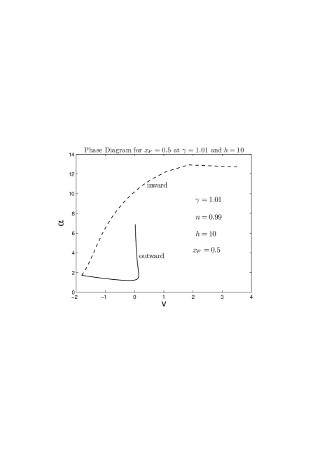
Figure 34: Density-speed phase diagram for $\gamma=1.01$, $n=0.99$, $h=10$ and a chosen meeting point $x_{F}=0.5$. The ‘inward curve’ is a phase curve by integrating inward from different $x$ along the magnetosonic critical curve to $x_{F}=0.5$ and the ‘outward curve’ is the phase curve integrating outward from smaller $x$ to reach the same $x_{F}$. There is no match in this phase diagram, because for small $x$ along the magnetosonic critical curve, the solution curve encounters the magnetosonic singular surface before reaching $x_{F}=0.5$.

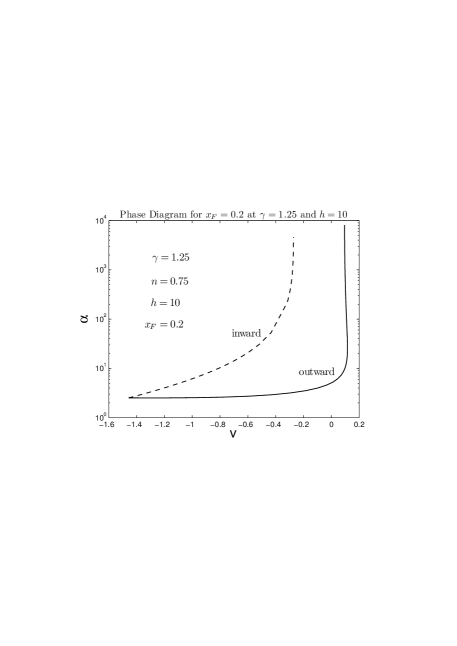
Figure 35: Density-speed phase diagram for $\gamma=1.25$, $n=0.75$, $h=10$ and a chosen meeting point $x_{F}=0.2$. The ‘inward curve’ is a phase curve obtained by integrating inward from different $x$ along the magnetosonic critical curve to reach $x_{F}$ and the ‘outward curve’ is a phase curve integrating outward from a smaller $x$. There is no solution match here.

For a stronger magnetic field with a larger $h$, no solution match can be found in the density-speed phase diagram. Figures 34 and 35 are two typical phase diagrams showing the two cases of $\gamma=1.01$, $n=0.99$, $h=10$ and of $\gamma=1.25$, $n=0.75$ and $h=10$, respectively. A possible interpretation of this feature is perhaps that for a large $h$, one can construct semi-complete solutions crossing the magnetosonic critical curve once as discussed in Section 4.3, while any outward solution curve will not reach the magnetosonic critical curve but continue to its lower left to infinity to match the asymptotic MHD solution (3.4.6).

5 Summary and Discussion

Table 8: The three corresponding parameters $A_{0}$, $B_{0}$ and $m(0)$ used in Figure 25 for hydrodynamic polytropic EECC solutions which are nearly isothermal.

Values of $\gamma=1.01$ and $h=0$.
No.	$A_{0}$	$B_{0}$	$m(0)$
1	5.200	1.883	0.3661
2	1.200	-0.7958	$4.7489\times 10^{-4}$
3	2.415	0.3145	$1.096\times 10^{-5}$
4	1.904	-0.09298	$6.6437\times 10^{-8}$

Table 9: The three corresponding parameters $A_{0}$, $B_{0}$ and $m(0)$ in Fig. 28 for MHD polytropic solutions which are nearly isothermal.

Values of $\gamma=1.01$ and $h=1$.
No.	$A_{0}$	$B_{0}$	$m(0)$
1	2.420	0.3719	$2.441\times 10^{-3}$
2	2.0155	-0.03997	$1.304\times 10^{-7}$
3	2.058	$3.868\times 10^{-3}$	$8.590\times 10^{-12}$

Table 10: The three corresponding parameters $A_{0}$, $B_{0}$ and $m(0)$ in Figs. 31 and 33.

Specified parameters are $\gamma=1.25$ and $n=0.75$.
$h$	$A_{0}$	$B_{0}$	$m(0)$
0	4.399	3.132	$2.243\times 10^{-2}$
1	5.894	2.267	$4.885\times 10^{-4}$

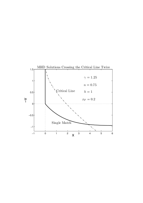
Figure 33: The single match of the similarity MHD solution for $\gamma=1.25$, $n=0.75$, $h=1$ and a chosen meeting point $x_{F}=0.2$, obtained with the two magnetosonic crossing points located at $x=3.8496$ ($\alpha=0.2087287$, $v=0.9027$) and $x=5.6384\times 10^{-5}$ ($\alpha=36912$, $v=-4.1624$) along the magnetosonic critical curve. This match is shown in the phase diagram of Fig. 32.

We developed an MHD formulation to describe a quasi-spherical symmetric gas cloud obeying a conventional polytropic equation of state in the presence of a random magnetic field and searched for various possible semi-complete MHD similarity solutions within this model framework. Here, we mainly focus on MHD effects of a random magnetic field; other effects such as diffusions and radiative diagnostics will be pursued in separate papers.

This formulation reveals several key MHD features of a gas cloud when a polytropic equation of state and a random magnetic field are combined together. First, the magnetosonic critical curve diverges when $x$ approaches zero, and may head up to the first quadrant in the $-v$ versus $x$ presentation when $h$ becomes sufficiently large. In the absence of a random magnetic field, the sonic critical curve also diverges as $x$ approaches zero. In the presence of a random magnetic field, the isothermal magnetosonic critical curve remains finite at $x=0$ (Yu and Lou, 2005; Yu et al., 2006). Therefore, this small $x$ diverging behaviour is fundamentally related to the polytropic approximation in contrast to the isothermal approximation. Secondly, for a sensible range of magnetic field strengths, the so-called mEWCSs may describe the large-scale MHD evolution of a magnetized gas cloud. But for too strong a random magnetic field, such a mEWCS does not exist. In this regard, our formalism is naturally applicable to a weakly magnetized gas cloud in large-scale outward and inward motions. For $B_{0}=0$, a magnetized gas cloud may have a tendency to expand as $h$ becomes sufficiently large. Thirdly, there exist additional MHD EECC solutions that cross the magnetosonic critical curve once with asymptotic MHD solution (3.4.6) at large $x$; these possible asymptotic MHD expansion solutions at large $x$ were not realized before (Lou and Shen, 2004; Hunter, 1977). We note that semi-complete or shock solutions matching with such asymptotic polytropic expansion solutions may be constructed without a random magnetic field with $h=0$. Fourthly, there exists a novel series asymptotic MHD solution (62) and (63) for small $x$ with a very dense core as well as a strong central magnetic field, and one can construct semi-complete self-similar MHD solutions using this asymptotic MHD solution. Finally, for $\gamma=1.25$ as an example of illustration, we have not observed the trend of spiral pattern in the density-speed phase diagram for solution matches. Therefore, there seem to be no trend of infinitely many semi-complete solutions crossing the critical curve twice under certain situations.

Our model analysis for a magnetized polytropic gas cloud requires the following assumptions: the magnetic field is locally random on small scales with a large-scale quasi-spherical symmetry Zel’dovich and Novikov (1971), the profiles of mass density, radial velocity, gas temperature and thermal pressure are all taken to possess a quasi-spherical symmetry on large scales. We impose these assumptions as the first approximation for a quasi-spherical magnetized gas medium, and we try to assess the role of a random magnetic field under such assumptions quantitatively and qualitatively. Our model analysis is specific and in details, while for astrophysical applications, we gain a physical sense qualitatively and should be careful with the adopted approximation and thus the model limitations. An important conceptual issue should be noted here. Even for a hydrodynamic flow of spherical symmetry in the absence of a random magnetic field, something must happen around the centre to destroy the self-similarity and the spherical symmetry except that a central black hole may accrete gas materials and absorb them in a smooth and quiet manner (e.g., Cai and Shu, 2005). For any other central objects such as neutron stars, white dwarfs, or main-sequence stars, spherical symmetric accretions will unavoidably lead to central activities. Therefore, a self-similar evolution of hydrodynamic gas flows is possible outside the influence sphere of central activities. Parallel to this physical rationale, an MHD inflow of quasi-spherical symmetry in the presence of a random magnetic field will eventually give rise to a central sphere of MHD activities. Again, we expect that a self-similar evolution of MHD gas flows is possible outside this influence sphere of central MHD activities.

In this analysis, we have adopted a polytropic equation of state (6). We note the existence of two different definitions for the term ‘polytropic’: one corresponds to an overall equation of state $p=\kappa\rho^{\gamma}$ with a constant $\kappa$ throughout the dynamic evolution in spatial and temporal domains (Goldreich and Weber, 1980), while the other corresponds to the entropy conservation along the streamline

$$\left(\frac{\partial}{\partial t}+u\frac{\partial}{\partial r}\right)\left[\log\left(\frac{p}{\rho^{\gamma}}\right)\right]=0\ ,$$ (108)

indicating that every infinitesimal portion of gas obeys the polytropic state equation along each streamline, but not necessarily in the global sense (e.g., Bouquet et al., 1985), i.e., the entropy per unit mass assigned to each streamline can be different. In the present flow problem, all streamlines are radial and a constant $\kappa$ for all streamlines would certainly meet the requirement of a quasi-spherical symmetry. In other words, we have taken the former, yet we recognize that if the latter is adopted, the parameter $n$ would be a free parameter, which may be adjusted to fit the requirements of, for examples, initial density profiles, initial ‘equations of state’ or asymptotic finite radial speeds at large $x$. By taking the former definition of a ‘polytropic’ gas, our analysis is primarily for the case of $n=2-\gamma$. In fact, Suto and Silk (1988) set the equation of state to be

$$p=\kappa(t)\rho^{\gamma}\ ,$$ (109)

where $\kappa(t)$ [corresponding to the notation $K(t)$ of Suto and Silk (1988)] takes the form of a power law in time $t$ to accommodate certain unknown energetic processes. This form of $\kappa(t)$ depending on $t$ constrains the range of index $\gamma$. If we adopt the usual polytropic equation of state from the perspective of Suto and Silk (1988), parameter $n$ should take on the value of $2-\gamma$. If instead, $\kappa$ is allowed to assume the form of power laws in both $t$ and $r$ and equation (109) is adopted, one more free parameter (equivalent to our parameter $n$ here) would emerge, as has been done for example by Cheng (1978) and Fatuzzo et al. (2004). For a careful study on behaviours of ‘polytropic’ gas under the latter definition, we should allow for the freedom of parameters in this problem and treat $\kappa$ as a function of both $r$ and $t$. In short, we have treated here only the case of $\gamma=2-n$ rather than $n=1$ (Suto and Silk, 1988).

Goldreich and Weber (1980) studied the specific case of $\gamma=4/3$, invoking this model to describe a homologous evolution of the core collapse of a supernova progenitor. Yahil (1983) noted that even for a slight departure of $\gamma$ value from the exact value $4/3$, the core collapse will be no longer completely homologous. At this stage, the results of Goldreich and Weber (1980) are beyond the framework of our study, because for $\gamma=4/3$, our similarity MHD transformation (3.1) becomes invalid. With this qualification, we briefly discuss limiting features of our model analysis as $\gamma$ approaches $4/3$. In our model framework, especially in reference to nonlinear MHD ODEs (3.2) and (24), parameter $n$ will approach $2/3$ as $\gamma\rightarrow 4/3$; it then follows that the factor $(nx-v)/(3n-2)$ goes to infinity, except when $v$ approaches $2x/3$ simultaneously, corresponding to a homologous collapse. Since first derivatives $v^{\prime}$ and $\alpha^{\prime}$ in terms of $x$ should remain finite in both MHD ODEs (3.2) and (24), we conclude that as $n$ approaches $2/3$, we must require $v=2x/3$ in order to avoid infinite first derivatives of both $v$ and $\alpha$. Therefore in our MHD case, a homologous collapse should still exist (see Yahil 1983 for an analysis of departure from $\gamma=4/3$). This argument serves only as a quick analysis and detailed calculations will be pursued in a separate paper.

The consequences of adopting a polytropic equation of state and incorporating a random magnetic field in our formulation of gas collapses and outflows lead to several novel features of possible MHD solutions in comparison to earlier analyses. Firstly, the new asymptotic MHD solutions (62) and (63) describe a gas cloud in which a random magnetic field and gas materials are both compressed in the core region with a very high total pressure in the core. This asymptotic MHD solution may represent a self-similar dynamic evolution course that forms a compact stellar object that contains extremely intense magnetic field and high mass density. The formation of this type of objects requires an embedded random magnetic field to be strong enough, because for $h=0$ this asymptotic solution for small $x$ does not exist (see Yu et al. 2006 for this type of asymptotic MHD solutions in an isothermal gas medium). Secondly, with or without a random magnetic field, the EECC solutions crossing the critical curve once provides a possibility that a gas cloud with a collapsing core has a much faster expanding envelope at a high radial speed. A more general treatment of flows at relativitistic speeds under a strong gravity would involve the general theory of relativity; in fact, the expanding envelope represents a kind of nonrelativistic Einstein-de Sitter expansion (Shu et al., 2002; Lou and Shen, 2004; Yu and Lou, 2005). Here, we further speculate the possibility that a random magnetic field and a polytropic equation of state might be relevant to the large-scale expansion of the entire universe involving a weak and random magnetic field. Finally, although MHD EECC solutions crossing the magnetosonic critical curve once can be constructed with a strong magnetic field, it can happen that the kind of EECC solutions crossing the critical curve twice (Lou and Shen, 2004) does not exist. The point is that the two MHD solutions having different asymptotic forms may not connect each other. In other words, it seems to be the case that for a very strong magnetic field, there are no semi-complete solutions to approach asymptotic MHD solutions (39) and (3.4.1) at large $x$. This is to say that for these cases, the MHD gas flow system does not have a non-increasing self-similar radial flow profile.

We now describe and comment on the self-similar oscillatory behaviour about the abscissa $x-$axis described in subsection 4.3, i.e., of the numerical solutions 1Ii, 2Ii and 3Ii in Figs. 17 and 18 for the hydrodynamic and MHD cases, respectively. Typically, the $-v$ versus $x$ solution curve behaves in the following manner. In the range of small $x$ values, $-v$ appears to cross the $x$-axis repeatedly and regularly for a number of infinite times, each cycle with a period decreasing with smaller $x$, and the vibrating amplitude also decreases as $x$ decreases in an apparent power-law fashion (see Fig. 36). We explored this feature down to $x\geq 10^{-20}$ and did not find the curve to crash on to the singular surface. An illustrating example of this vibration behaviour is clearly shown in Fig. 36. This behaviour, after careful examination and comparison of numerical and analytical results, turns out to be the type II ‘quasi-static’ asymptotic solution derived by Lou and Wang (2006) where the hydrodynamic problem in the absence of magnetic field was solved. Appendix G gives a brief account of the basic results. This behaviour is a characteristic of the polytropic equation of state with or without magnetic field. However as shown in Appendix G, the presence of a magnetic field modifies the asymptotic solution behaviour in a non-trivial manner.

Appendix A Magnetic Induction and the Lorentz Force

In this appendix, we rearrange the magnetic induction equation and discuss approximations made regarding the magnetic Lorentz force in our MHD formulation with the simplification of a quasi-spherical symmetry on large scales (Yu and Lou, 2005; Yu et al., 2006).

For non-relativistic quasi-neutral MHD flows, the magnetic Lorentz force density can be split into two terms

$$\frac{(\nabla\times\overrightarrow{B})\times\overrightarrow{B}}{4\pi}=-\nabla\bigg{(}\frac{B^{2}}{8\pi}\bigg{)}+\frac{(\overrightarrow{B}\cdot\nabla)\overrightarrow{B}}{4\pi}\$$ (110)

by a vector identity and the $\nabla\cdot\vec{B}=0$ condition. The first and second terms on the RHS represent the magnetic pressure and tension force densities. The radial component of the magnetic tension force on the RHS is

$$\frac{1}{4\pi}\bigg{[}B_{r}\frac{\partial B_{r}}{\partial r}+\frac{B_{\theta}}{r}\frac{\partial B_{r}}{\partial\theta}+\frac{B_{\phi}}{r\sin\theta}\frac{\partial B_{r}}{\partial\phi}-\frac{(B_{\theta}^{2}+B_{\phi}^{2})}{r}\bigg{]}\ ,$$ (111)

where the first term in the square brackets cancels a relevant term of the magnetic pressure force in expression (110). For a large-scale average of a random magnetic field, we assume $<B_{\theta}\cdot\partial B_{r}/\partial r>\cong 0$ and $<B_{\phi}\cdot\partial B_{r}/\partial\theta>\cong 0$. The nonvanishing radial component of the magnetic Lorentz force density associated with the mean square of the random transverse magnetic field is

$$-\frac{\partial}{\partial r}\bigg{(}\frac{<B_{t}^{2}>}{8\pi}\bigg{)}-\frac{<B_{t}^{2}>}{4\pi r}\$$ (112)

as shown in equation (4).

In the absence of resistivity and ambipolar diffusions etc., the magnetic induction equation appears as

$$\frac{\partial\overrightarrow{B}}{\partial t}=\nabla\times(\overrightarrow{v}\times\overrightarrow{B})\ ,$$ (113)

which can be written explicitly in three component forms in spherical polar coordinates $(r,\theta,\phi)$, viz.,

$$\frac{\partial B_{r}}{\partial t} = \frac{1}{r\sin\theta}\frac{\partial}{\partial\theta}\bigg{[}\sin\theta(v_{r}B_{\theta}-v_{\theta}B_{r})\bigg{]}$$ (114)

$$-\frac{1}{r\sin\theta}\frac{\partial}{\partial\phi}(v_{\phi}B_{r}-v_{r}B_{\phi})\ ,$$

$$\frac{\partial B_{\theta}}{\partial t} = \frac{1}{r\sin\theta}\frac{\partial}{\partial\phi}(v_{\theta}B_{\phi}-v_{\phi}B_{\theta})$$ (115)

$$-\frac{1}{r}\frac{\partial}{\partial r}\bigg{[}r(v_{r}B_{\theta}-v_{\theta}B_{r})\bigg{]}\ ,$$

$$\frac{\partial B_{\phi}}{\partial t} = \frac{1}{r}\frac{\partial}{\partial r}\bigg{[}r(v_{\phi}B_{r}-v_{r}B_{\phi})\bigg{]}$$ (116)

$$-\frac{1}{r}\frac{\partial}{\partial\theta}(v_{\theta}B_{\phi}-v_{\phi}B_{\theta})\ .$$

In the approximation of quasi-spherical symmetry, we take $<v_{\theta}>\cong 0$ and $<v_{\phi}>\cong 0$. The $\theta-$ and $\phi-$components of the magnetic induction equation can thus be simplified to the following forms of

$$\frac{\partial B_{\theta}}{\partial t}=-\frac{1}{r}\frac{\partial}{\partial r}(rv_{r}B_{\theta})\ ,$$ (117)

$$\frac{\partial B_{\phi}}{\partial t}=-\frac{1}{r}\frac{\partial}{\partial r}(rv_{r}B_{\phi})\ ,$$ (118)

which then immediately lead to

$$\frac{\partial}{\partial t}\bigg{(}\frac{r^{2}B_{t}^{2}}{2}\bigg{)}+\frac{v_{r}}{2}\frac{\partial}{\partial r}(r^{2}B_{t}^{2})+r^{2}B_{t}^{2}\frac{v_{r}}{r}=0\ ,$$ (119)

where $B_{t}^{2}\equiv B_{\theta}^{2}+B_{\phi}^{2}$ is proportional to the energy density of the random transverse magnetic field. Equation (119) is simply the magnetic induction equation (5). For the radial component of the magnetic induction equation (Yu and Lou, 2005; Yu et al., 2006), we have approximately

$$\frac{\partial(r^{2}B_{r})}{\partial t}+v_{r}\frac{\partial(r^{2}B_{r})}{\partial r}=r^{2}(\overrightarrow{B}_{t}\cdot\nabla)v_{r}\ .$$ (120)

Equations (119) and (120) here differ from equations (1’) and (1) in the formulation of Chiueh and Chou (1994).

Appendix B Partial Derivatives of $A$, $V$ and $X$

The first-order partial derivatives of $A$, $V$ and $X$ as functions of $\alpha$, $v$, and $x$ are used in subsection 3.6. They are derived from expressions (3.2), (3.2), and (27) for $A$, $V$ and $X$, respectively, with straightforward manipulations. We present below the explicit expressions of these partial derivatives, which are used in numerical integrations to determine the MHD solution behaviours in the vicinity of the sonic or magnetosonic critical curves.

$$A_{\alpha}= 2\alpha\bigg{[}(n-1)v-\frac{2(x-v)(nx-v)}{x}\bigg{]}$$ (121)

$$+3\alpha^{2}\bigg{[}2hx+\frac{(nx-v)}{(3n-2)}\bigg{]}\ ,$$

$$A_{v}=\alpha^{2}\bigg{[}3n+1-\frac{\alpha}{(3n-2)}-\frac{4v}{x}\bigg{]}\ ,$$ (122)

$$A_{x}=\alpha^{2}\bigg{[}\bigg{(}2h+\frac{n}{3n-2}\bigg{)}\alpha-2n+\frac{2v^{2}}{x^{2}}\bigg{]}\ ,$$ (123)

$$V_{\alpha}= (n-1)\big{[}v(nx-v)+4h\alpha x^{2}\big{]}$$ (124)

$$+\frac{2(nx-v)^{2}}{(3n-2)}\alpha-2\gamma^{2}\alpha^{\gamma-1}\frac{(x-v)}{x}\ ,$$

$$V_{v}=(n-1)\big{(}nx-2v\big{)}\alpha-\frac{2\alpha^{2}(nx-v)}{(3n-2)}+\frac{2\gamma\alpha^{\gamma}}{x}\ ,$$ (125)

$$V_{x}=(n-1)\big{(}nv+4h\alpha x\big{)}\alpha+\frac{2n\alpha^{2}(nx-v)}{(3n-2)}-\frac{2\gamma\alpha^{\gamma}v}{x^{2}}\ ,$$ (126)

$$X_{\alpha}=(nx-v)^{2}-\gamma^{2}\alpha^{\gamma-1}-2h\alpha x^{2}\ ,$$ (127)

$$X_{v}=-2\alpha(nx-v)\ ,$$ (128)

$$X_{x}=2n\alpha(nx-v)-2h\alpha^{2}x\ .$$ (129)

Appendix C Second-Order Derivatives of $\alpha(x)$ and $\mathit{v(x)}$

For nodal points referred to in subsection 3.6, there are infinitely many solutions crossing the sonic and magnetosonic critical curves. Only the analytical eigensolutions determined by equations (100), (101) and (3.6) are of main interest here, and a numerical integration is unstable in the direction away from the critical curve if one uses only the first-order derivatives of $\alpha(x)$ and $v(x)$ with respect to $x$. So one should work out the second-order derivatives of $\alpha(x)$ and $v(x)$ with respect to $x$ in order to pick out the analytic eigensolutions among many other solutions having weak discontinuities across the sonic or magnetosonic critical curves (Lazarus, 1981; Whitworth and Summers, 1985; Hunter, 1986). These weak discontinuities may be regarded as weak shocks (Boily and Lynden-Bell, 1995). It is also possible to construct various forms of shocks across the sonic or magnetosonic critical curve (Tsai and Hsu, 1995; Shu et al., 2002; Shen and Lou, 2004; Bian and Lou, 2005; Yu and Lou, 2006; Lou and Wang, 2006, 2007).

We determine the second-order derivatives of $\alpha(x)$ and $v(x)$ with respect to $x$ by the following procedure. As $A=V=X=0$ along the sonic or magnetosonic critical curve, one readily obtains

$$\alpha^{\prime\prime}=\frac{X^{\prime}A^{\prime\prime}-X^{\prime\prime}A^{\prime}}{2(X^{\prime})^{2}}=\frac{A^{\prime\prime}-\alpha^{\prime}X^{\prime\prime}}{2X^{\prime}}\ ,$$ (130)

$$v^{\prime\prime}=\frac{X^{\prime}V^{\prime\prime}-X^{\prime\prime}V^{\prime}}{2(X^{\prime})^{2}}=\frac{V^{\prime\prime}-v^{\prime}X^{\prime\prime}}{2X^{\prime}}\ .$$ (131)

We denote the second derivatives of $A$, $V$ and $X$ as

$$\left(\begin{matrix}A^{\prime\prime}\cr V^{\prime\prime}\cr X^{\prime\prime}\cr\end{matrix}\right)=\textbf{F}\left(\begin{matrix}\alpha^{\prime\prime}\cr v^{\prime\prime}\cr 1\cr\end{matrix}\right)=\left(\begin{matrix}f_{11}&f_{12}&f_{13}\cr f_{21}&f_{22}&f_{23}\cr f_{31}&f_{32}&f_{33}\cr\end{matrix}\right)\left(\begin{matrix}\alpha^{\prime\prime}\cr v^{\prime\prime}\cr 1\cr\end{matrix}\right)\ ,$$ (132)

where each matrix element $f_{ij}=f_{ij}(\alpha,v,x,\alpha^{\prime},v^{\prime})$ of matrix F is a function of $\alpha$, $v$, $x$, $\alpha^{\prime}$ and $v^{\prime}$ ($i,j=1,2,3$). Substituting equation (132) into equations (130) and (131), one immediately obtains

$$(2X^{\prime}+\alpha^{\prime}f_{31}-f_{11})\alpha^{\prime\prime}+(\alpha^{\prime}f_{32}-f_{12})v^{\prime\prime}=f_{13}-\alpha^{\prime}f_{33}\ ,$$ (133)

$$(v^{\prime}f_{31}-f_{21})\alpha^{\prime\prime}+(2X^{\prime}+v^{\prime}f_{32}-f_{22})v^{\prime\prime}=f_{23}-v^{\prime}f_{33}\ ,$$ (134)

from which $\alpha^{\prime\prime}$ and $v^{\prime\prime}$ can be solved directly for the nondegenerate case and be expressed and computed by corresponding $x$, $\alpha$, $v$ $\alpha^{\prime}$ and $v^{\prime}$ at points along the magnetosonic critical curve. For the convenience of reference and checking, we summarize the explicit expressions for functions $X^{\prime}$ and $f_{ij}$ below.

$$X^{\prime}=(nx-v)^{2}\alpha^{\prime}+2\alpha(nx-v)(n-v^{\prime})\qquad$$

$$-\gamma^{2}\alpha^{\gamma-1}\alpha^{\prime}-2h\alpha^{2}x-2h\alpha x^{2}\alpha^{\prime}\ ,$$ (135)

$$f_{11}\equiv\alpha^{2}\bigg{[}2hx+\frac{(nx-v)}{(3n-2)}\bigg{]}\ ,$$ (136)

$$f_{12}\equiv\alpha^{2}\bigg{[}3n+1-\frac{4v}{x}-\frac{\alpha}{(3n-2)}\bigg{]}\ ,$$ (137)

$$f_{13}\equiv 4\alpha\alpha^{\prime}\bigg{[}(3n+1)v^{\prime}+\bigg{(}2h+\frac{n-v^{\prime}}{3n-2}\bigg{)}\alpha\qquad$$

$$+\bigg{(}2hx+\frac{nx-v}{3n-2}\bigg{)}\alpha^{\prime}-2n-\frac{2v}{x^{2}}(2xv^{\prime}-v)\bigg{]}$$

$$+\alpha^{2}\bigg{[}2\bigg{(}2h+\frac{n-v^{\prime}}{3n-2}\bigg{)}\alpha^{\prime}-\frac{4}{x^{3}}(v-xv^{\prime})^{2}\bigg{]}\ ,$$ (138)

$$f_{21}\equiv(n-1)\big{[}v(nx-v)+4h\alpha x^{2}\big{]}\qquad$$

$$+2\alpha\frac{(nx-v)^{2}}{3n-2}-2\gamma^{2}\alpha^{\gamma-1}\frac{(x-v)}{x}\ ,\qquad$$ (139)

$$f_{22}\equiv(n-1)\alpha(nx-2v)-\frac{2\alpha^{2}(nx-v)}{3n-2}+\frac{2\gamma\alpha^{\gamma}}{x}\ ,$$ (140)

$$f_{23}\equiv(n-1)\bigg{[}2(\alpha v^{\prime}+v\alpha^{\prime})(n-v^{\prime})\qquad$$

$$+2(nx-v)\alpha^{\prime}v^{\prime}+4h\alpha^{2}+16h\alpha x\alpha^{\prime}+4hx^{2}(\alpha^{\prime})^{2}\bigg{]}$$

$$+2\frac{(nx-v)^{2}}{(3n-2)}(\alpha^{\prime})^{2}+\frac{8\alpha(nx-v)(n-v^{\prime})\alpha^{\prime}}{(3n-2)}$$

$$+\frac{2\alpha^{2}(n-v^{\prime})^{2}}{(3n-2)}-2\gamma^{2}(\gamma-1)\alpha^{\gamma-2}\frac{(x-v)}{x}(\alpha^{\prime})^{2}$$

$$-4\gamma^{2}\alpha^{\gamma-1}\alpha^{\prime}\frac{(v-xv^{\prime})}{x^{2}}-4\gamma\alpha^{\gamma}\frac{(xv^{\prime}-v)}{x^{3}}\ ,$$ (141)

$$f_{31}\equiv(nx-v)^{2}-\gamma^{2}\alpha^{\gamma-1}-2hx^{2}\alpha\ ,$$ (142)

$$f_{32}\equiv-2\alpha(nx-v)\ ,$$ (143)

$$f_{33}\equiv 4(nx-v)\alpha^{\prime}(n-v^{\prime})+2\alpha(n-v^{\prime})^{2}-2h\alpha^{2}\qquad$$

$$-\gamma^{2}(\gamma-1)\alpha^{\gamma-2}(\alpha^{\prime})^{2}-8h\alpha x\alpha^{\prime}-2hx^{2}(\alpha^{\prime})^{2}\ .$$

Appendix D A Proof of $D_{3}=0$

We conclude that because the magnetosonic critical curve is a continuous curve as we have solved it analytically, it must lead to $D_{3}=0$ in cubic equation (106). A brief proof is presented below. Since functionals $A,\ V,\ X$ as defined by equations $(\ref{wang77})-(\ref{wang79})$ together determine the magnetosonic critical curve (i.e., setting $A=V=X=0$ simultaneously), we begin by assuming that the point $(\alpha_{1},\ v_{1},\ x_{1})$ in the $\alpha-v-x$ space is on the magnetosonic critical curve such that $K(\alpha_{1},\ v_{1},\ x_{1})=0$ where $K$ denotes $A$, $V$ or $X$, respectively. We further assume that the set $(\alpha_{1}+\delta\alpha\ ,v_{1}+\delta v\ ,x_{1}+\delta x)$ is also along the magnetosonic critical curve and is very near to the former point. Then from the requirement $K(\alpha_{1}+\delta\alpha\ ,v_{1}+\delta v\ ,x_{1}+\delta x)=0$, with $K$ denoting $A$, $V$ and $X$ as appropriate, we infer that $\delta K\equiv K(\alpha_{1}+\delta\alpha,\ v_{1}+\delta v,\ x_{1}+\delta x)-K(\alpha_{1},\ v_{1},\ x_{1})=0$. It then follows from

$$\delta K=\frac{\partial K}{\partial\alpha}\delta\alpha+\frac{\partial K}{\partial v}\delta v+\frac{\partial K}{\partial x}\delta x\ ,$$ (145)

with $K$ denoting $A$, $V$ or $X$ in turn, that

$$\left(\begin{matrix}A_{\alpha}&A_{v}&A_{x}\cr V_{\alpha}&V_{v}&V_{x}\cr X_{\alpha}&X_{v}&X_{x}\cr\end{matrix}\right)\left(\begin{matrix}\delta\alpha\cr\delta v\cr\delta x\end{matrix}\right)=0$$ (146)

along the magnetosonic critical curve for the given set of $(\alpha_{1},\ v_{1},\ x_{1})$. For a nontrivial set of $(\delta\alpha,\ \delta v,\ \delta x)$, we must then require

$$\left|\begin{matrix}A_{\alpha}&A_{v}&A_{x}\cr V_{\alpha}&V_{v}&V_{x}\cr X_{\alpha}&X_{v}&X_{x}\cr\end{matrix}\right|=0\$$ (147)

along the magnetosonic critical curve, which is clearly equivalent to $D_{3}=0$ in cubic equation (106).

Appendix E Determination of Magnetosonic Critical Curves

Table 11: Algebraic signs for quantities $A_{1}$, $B_{1}$, $C_{1}$ and $\Delta$, and the corresponding root numbers for a usual polytropic gas with $\gamma=1.01$ and $n=0.99$

$\gamma=1.01$,     $n=0.99$,     $h=0$
$\alpha_{11}=0.202728\ ,\ \ \ \alpha_{12}=0.282682$
$\alpha\in$	$(0\ ,\ \alpha_{11})$	$(\alpha_{11}\ ,\ \alpha_{12})$	$(\alpha_{12}\ ,\ +\infty)$
signs		$B_{1}>0$	$B_{1},\ \Delta>0$
	all$\ <0$	others$\ <0$	$A_{1},\ C_{1}<0$
root No.	0	0	2

$\gamma=1.01$,    $n=0.99$,    $h=0.1$
$\alpha_{21}=0.048500,\ \alpha_{22}=0.103907,\ \alpha_{23}=0.202728$
$\alpha\in$	$(0,\ \alpha_{21})$	$(\alpha_{21},\ \alpha_{22})$	$(\alpha_{22},\ \alpha_{23})$	$(\alpha_{23},\ +\infty)$
signs		$\Delta>0$	$A_{1},\ \Delta>0$	$A_{1},\ B_{1},\ \Delta>0$
	all$\ <0$	others$\ <0$	$B_{1},\ C_{1}<0$	$C_{1}<0$
root No.	0	0	1	1

$\gamma=1.01$,     $n=0.99$,     $h=1$
$\alpha_{31}=4.9485\times 10^{-3},\ \alpha_{32}=0.051866,\ \alpha_{33}=0.202728$
$\alpha\in$	$(0,\ \alpha_{31})$	$(\alpha_{31},\ \alpha_{32})$	$(\alpha_{32},\ \alpha_{33})$	$(\alpha_{33},\ +\infty)$
signs		$\Delta>0$	$\!\!\!A_{1},\Delta>0$	$\!\!\!\!\!A_{1},B_{1},\Delta>0$
	all$\ <0$	others$\ <0$	$B_{1},C_{1}<0$	$C_{1}<0$
root No.	0	$\!\!\!0$	$\!\!\!1$	$\!\!\!1$

$\gamma=1.01$,     $n=0.99$,     $h=10$
$\alpha_{41}=4.9440\times 10^{-4},\ \alpha_{42}=0.027885,\ \alpha_{43}=0.202728$
$\!\!\!\alpha\in$	$(0,\ \alpha_{41})$	$(\alpha_{41},\ \alpha_{42})$	$(\alpha_{42},\ \alpha_{43})$	$(\alpha_{43},\ +\infty)$
signs		$\Delta>0$	$\!\!\!A_{1},\Delta>0$	$\!\!\!A_{1},B_{1},\Delta>0$
	all$\ <0$	others$\ <0$	$B_{1},C_{1}<0$	$C_{1}<0$
root No.	0	0	1	1

Table 12: Algebraic signs for quantities $A_{1}$, $B_{1}$, $C_{1}$ and $\Delta$, and the corresponding root numbers for a polytropic gas with $\gamma=1.25$ and $n=0.75$

$\gamma=1.25\ ,$   $n=0.75\ ,$   $h=0$
$\alpha_{51}=0.279006\ ,\ \ \alpha_{52}=0.368686$
$\alpha\in$	$(0\ ,\ \alpha_{51})$	$(\alpha_{51}\ ,\ \alpha_{52})$	$(\alpha_{53}\ ,\ +\infty)$
signs		$B_{1}>0$	$B_{1}\ ,\ \Delta>0$
	all$\ <0$	others$\ <0$	$A_{1}\ ,\ C_{1}<0$
root No.	0	0	2

$\gamma=1.25$,    $n=0.75$,    $h=1$
$\alpha_{61}=0.09283\ ,\ \alpha_{62}=0.174661\ ,\ \alpha_{63}=0.279006$
$\alpha\in$	$(0,\ \alpha_{61})$	$(\alpha_{61},\ \alpha_{62})$	$(\alpha_{62},\ \alpha_{63})$	$(\alpha_{63},\ +\infty)$
signs		$\Delta>0$	$A_{1},\Delta>0$	$A_{1},B_{1},\Delta>0$
	all$\ <0$	others$\ <0$	$B_{1},C_{1}<0$	$C_{1}<0$
root No.	0	0	1	1

$\gamma=1.25$,    $n=0.75$,    $h=10$
$\alpha_{71}=0.0090897\ ,\ \alpha_{72}=0.107674\ ,\ \alpha_{73}=0.279006$
$\alpha$	$(0\ ,\alpha_{71})$	$(\alpha_{71}\ ,\ \alpha_{72})$	$(\alpha_{72}\ ,\ \alpha_{73})$	$(\alpha_{73}\ ,\ +\infty)$
signs		$\!\!\!\!\Delta>0$	$\!\!\!\!A_{1},\Delta>0$	$\!\!\!\!A_{1},B_{1},\Delta>0$
	all$\ <0$	others$\ <0$	$B_{1}\ ,\ C_{1}<0$	$C_{1}<0$
root No.	0	0	1	1

$\gamma=1.25$,    $n=0.75$,    $h=100$
$\alpha_{81}=8.9955\times 10^{-4}\ ,\ i\alpha_{82}=7.1799\times 10^{-3}\ ,\ \alpha_{83}=0.038660$
$\alpha\in$	$(0\ ,\ \alpha_{81})$	$(\alpha_{81}\ ,\ \alpha_{82})$	$(\alpha_{82}\ ,\ \alpha_{83})$
signs		$\Delta>0$	$A_{1}\ ,\ \Delta>0$
	all$\ <0$	others$<0$	$B_{1}\ ,\ C_{1}<0$
root No.	0	0	1
$\alpha_{84}=0.079160\ ,\ \ \alpha_{85}=0.279006$
$\alpha\in$	$(\alpha_{83}\ ,\ \alpha_{84})$	$(\alpha_{84}\ ,\ \alpha_{85})$	$(\alpha_{85}\ ,\ +\infty)$
signs	$\Delta>0$	$A_{1}\ ,\ \Delta>0$	$A_{1},\ B_{1},\ \Delta>0$
	others$\ <0$	$B_{1}\ ,\ C_{1}<0$	$C_{1}<0$
root No.	0	1	1

One can numerically determine ranges of $\alpha$ values for which the signs of $A_{1}$, $B_{1}$ and $C_{1}$ and of the determinant $\Delta\equiv B_{1}^{2}-4A_{1}C_{1}$ in equation (35) do not change and one can thus decide which root of $x^{2}$ should be picked up in equation (34) and how many roots are physically relevant once specific values of $\gamma$, $h$ and $n$ are prescribed. This numerical exploration is important as one needs to know the sonic or magnetosonic critical curve in the entire range of $0^{+}<\alpha<+\infty$. We have analyzed the usual polytropic cases of $\gamma=1.01$, $n=0.99$ and $\gamma=1.25$, $n=0.75$ for different $h$ values. Here, we summarize the main results. The case that $\gamma=1.01$ and $n=0.99$ is contained in Table 11 and the case that $\gamma=1.25$ and $n=0.75$ is contained in Table 12.

Appendix F MHD Eigensolution Behaviours in the Vicinity of the Magnetosonic Critical Curve

Table 13: Algebraic signs of both determinant $\Delta\equiv B_{3}^{2}-4C_{3}$ and $C_{3}$ for equation (106) and type identifications for local behaviours of MHD eigensolutions in the vicinity of magnetosonic critical curves for a conventional polytropic gas with $\gamma=1.01$ and $n=0.99$, where ‘s’, ‘n’ and ‘c’ denote a saddle, node, and a centre (or spiral), respectively (Jordan and Smith, 1977).

$\gamma=1.01$,    $n=0.99$,    $h=0$
$x_{11}=1.0455\ ,\ \ \ x_{12}=47.31$
$x\in$	$(0\ ,\ x_{11})$	$(x_{11}\ ,\ x_{12})$	$(x_{12}\ ,\ +\infty)$
signs	$\Delta>0$	$\Delta\ ,\ C_{3}>0$	$C_{3}>0$
	$C_{3}<0$		$\Delta<0$
type identification	s	n	c

$\gamma=1.01$,  $n=0.99$,  $h=0.1$
$x_{21}=1.1497$
$x\in$	$(0\ ,\ x_{21})$	$(x_{21}\ ,\ +\infty)$
signs	$\Delta>0$	$\Delta\ ,\ C_{3}>0$
	$C_{3}<0$
type identification	s	n

$\gamma=1.01$,    $n=0.99$,    $h=1$
$x_{31}=1.9182$
$x\in$	$(0\ ,\ x_{31})$	$(x_{31}\ ,\ +\infty)$
signs	$\Delta>0$	$\Delta\ ,\ C_{3}>0$
	$C_{3}<0$
type identification	s	n

Table 14: Algebraic signs of both determinant $\Delta\equiv B_{3}^{2}-4C_{3}$ and $C_{3}$ for equation (106) and type identifications for local behaviours of MHD eigensolutions for a conventional polytropic gas in the vicinity of magnetosonic critical curves as $\gamma=1.25$ and $n=0.75$, where ‘s’, ‘n’, and ‘c’ denote saddle, node, and centre (or spiral), respectively (Jordan and Smith, 1977).

$\gamma=1.25$,     $n=0.75$,     $h=0$
$x_{41}=11.724\ ,\ \ \ \ x_{42}=11.724$
$x$	$(0\ ,\ x_{41})$	$(x_{41}\ ,\ x_{42})$	$(x_{42}\ ,\ +\infty)$
signs	$\Delta>0$	$\Delta\ ,\ C_{3}>0$	$C_{3}>0$
	$C_{3}<0$		$\Delta<0$
type identification	s	n	c

Similarity MHD solution behaviours in the vicinity of the magnetosonic critical curve can be determined by the signs of both $\Delta\equiv B_{3}^{2}-4C_{3}$ and $C_{3}$ as defined by equation (106) (see subsection 3.6 for details). One can numerically determine the values of $\Delta$ and $C_{3}$ given specific $x$ values of different magnetosonic critical curves corresponding to different parameter sets of $\gamma$, $n$ and $h$. We describe the main results of this exploration for the cases of $\gamma=1.01$, $n=0.99$ and $\gamma=1.25$, $n=0.75$ with different $h$ values. In Table 13, we present the relevant results for $\gamma=1.01$ and $n=0.99$, while in Table 14, we show the results for $\gamma=1.25$ and $n=0.75$. In both Tables 13 and 14, the sign ‘s’ indicates a saddle, ‘n’ indicates a node, and ‘c’ indicates a centre or a spiral regarded as being unphysical (Jordan and Smith, 1977). Note in particular that among the cases we have explored and not displayed in the above Tables, there exist such magnetosonic critical curves that all points along the lines are saddle points. These include the cases of $\gamma=1.01$, $n=0.99$, $h=10$ and $100$, and of $\gamma=1.25$, $n=0.75$, $h=1$, $10$, and $100$. There are also cases of $h>0$ with the coexistence of nodal, saddle and spiral or centre points along the magnetosonic curve, e.g., the case of $\gamma=1.01$, $n=0.99$ and $h=0.0001$. The fact that there exist spiral or centre points in unmagnetized cases should be noted because there would be no global semi-complete smooth solution crossing such points (subsection 3.6).

Appendix G Asymptotic Behaviours Approaching the Quasi Magnetostatic Solution

As mentioned above, global magnetostatic solution (74) also serves as an asymptotic behaviour for small $x$. This asymptotic solution turns out to be the only solution characterized by a $v$ approaching zero faster than ${\cal O}(x)$ and $\alpha\simeq x^{-2/n}$ when $n=2-\gamma$ for a usual polytropic gas. In order to determine the behaviour of this asymptotic solution, we assume to the leading order

$$v=Lx^{K}+\cdots\ ,$$ (148)

$$\alpha=\bigg{[}\frac{(2-\gamma)^{2}}{2\gamma(4-3\gamma)}+\frac{(1-\gamma)}{\gamma}h\bigg{]}^{1/(\gamma-2)}x^{-2/(2-\gamma)}+\Delta\alpha+\cdots\ ,$$

where the next-order $\alpha$ variation $\Delta\alpha$ is given by

$$\Delta\alpha=Nx^{K-1-2/n}\ ,$$ (149)

and $L$, $K$ and $N$ are three constant complex coefficients. Apparently, $Re(K)>1$ is required for $v$ to approach zero faster than $\sim{\cal O}(x)$ and $\Delta\alpha$ being the next-order term of this asymptotic solution as $x$ approaches zero.

Substituting asymptotic expressions (148) and (149) into nonlinear MHD ODEs (11) and (3.1) and using integral relation (21), we obtain the following two relations

$$\bigg{[}\frac{n^{2}(1+K)}{2(3n-2)}+nhK-\gamma h\bigg{]}N$$

$$=\bigg{[}\frac{n^{2}}{2\gamma(3n-2)}+\frac{(1-\gamma)}{\gamma}h\bigg{]}^{-1/n}\frac{L}{(3n-2)}\ ,$$

$$\frac{n(K-1)N}{(K-2-2/n)}=\bigg{[}\frac{n^{2}}{2\gamma(3n-2)}+\frac{(1-\gamma)}{\gamma}h\bigg{]}^{-1/n}L\$$ (150)

among the three complex constants $K$, $L$ and $N$. Clearly, $K$ satisfies the following quadratic equation

$$f(K)\equiv[n^{2}/2+n(3n-2)h]K^{2}$$

$$-(4-3n)[n/2+(3n-2)h]K$$

$$+n^{2}+\gamma(2/n-2)(3n-2)h=0\ .\qquad$$ (151)

Once a proper root of $K$ is chosen, the complex ratio of $L$ to $N$ is determined accordingly. We emphasize that the values of $N$ and $L$ are not determined a priori, i.e., $L$ can take on any reasonable value, while $N$ is determined by their ratio or vice versa.

We introduce the handy notation

$$h_{0} = \frac{\big{[}(3+2\sqrt{2})n-4\big{]}\big{[}4-(3-2\sqrt{2})n\big{]}}{2n(3n-2)}$$ (152)

$$= \frac{(1-n)(-n^{2}+24n-16)}{n^{3}}h_{c}\$$

and reach the following conclusions. When $12-8\sqrt{2}<n<0.8$ and $h_{0}<h<h_{c}$, or when $2/3<n<12-8\sqrt{2}$ for arbitrary $h$ values, there exist two real roots of $f(K)$, both are larger than unity; these are referred to as type I ‘quasi-static’ asymptotic solutions. When $12-8\sqrt{2}<n<0.8$ and $h<h_{0}$, there exists a complex root $K$ with its real part larger than unity; this is referred to as type II ‘quasi-static’ asymptotic solution. For a complex $K=K_{1}+iK_{2}$, we simply have

$$v=Lx^{K_{1}}x^{iK_{2}}=Lx^{K_{1}}\exp(iK_{2}\ln x)\ .$$ (153)

In the limit of $h=0$, the above MHD results reduce to those of a hydrodynamic analysis (Lou and Wang, 2006).

When $n\neq 2-\gamma$ for an unconventional polytropic gas, an asymptotic similarity MHD solution in the form of $v\simeq{\cal O}(x)$ and $\alpha\simeq x^{-2/(2-\gamma)}$ also exists, viz.

$$v=\frac{2(2-\gamma-n)}{(4-3\gamma)}x+\cdots\ ,$$

$$\alpha=\bigg{[}\frac{(1-\gamma)}{\gamma}h + \frac{(2-\gamma)}{\gamma(3n-2)}\bigg{(}\frac{n}{2}-\frac{2-\gamma-n}{4-3\gamma}\bigg{)}\bigg{]}^{-1/(2-\gamma)}$$ (154)

$$\times x^{-2/(2-\gamma)}+\cdots\ .$$

References

- (1) Bagchi, J., Durret, F., Neto, G. B. L., Paul, S.: Science 314, 791 (2006)
- (2) Barenblatt, G. I., Zel’dovich, Ya. B.: AnRFM 4, 285 (1972)
- (3) Bian F.-Y., Lou, Y.-Q.: MNRAS 363, 1315 (2005)
- (4) Bodenheimer, P., Sweigart, A.: ApJ 152, 515 (1968)
- (5) Boily, C. M., Lynden-Bell, D.: MNRAS 276, 133 (1995)
- (6) Bouquet, S., Feix, M. R., Fualkow, E., Munier, A.: ApJ 293, 494 (1985)
- (7) Cai, M. J., Shu, F. H.: ApJ 618, 438 (2005)
- (8) Cheng, A. F.: ApJ 221, 320 (1978)
- (9) Chiueh, T., Chou, J.-K.: ApJ 431, 380 (1994)
- (10) Fan, Z.H., Lou, Y.-Q.: MNRAS 307, 645 (1999)
- (11) Fatuzzo, M., Adams, F. C., Myers, P. C.: ApJ 615, 813 (2004)
- (12) Fillmore, J. M., Goldreich, P.: ApJ 284, 1 (1984)
- (13) Foster, P. N., Chevalier, R. A.: ApJ 416, 303 (1993)
- (14) Goldreich, P., Weber, S. V.: ApJ 238, 991 (1980)
- (15) Hanawa, T., Matsumoto, T.: ApJ 521, 703 (1999)
- (16) Hanawa, T., Matsumoto, T.: PASJ 52, 241 (2000)
- (17) Hanawa, T., Nakayama, K.: ApJ 484, 238 (1997)
- (18) Hennebelle, P.: A&A 397, 381 (2003)
- (19) Hu, J., Lou, Y.-Q.: ApJ 606, L1 (2005)
- (20) Hu, J., Shen, Y., Lou, Y.-Q., Zhang, S.-N.: MNRAS 365, 345 (2005)
- (21) Hunter, C.: ApJ 218, 834 (1977)
- (22) Hunter, C.: MNRAS 223, 391 (1986)
- (23) Inutsuka, S., Miyama, S. M.: ApJ 388, 392 (1992)
- (24) Jordan, D. W., Smith, P.: Nonlinear Ordinary Differential Equations, Oxford University Press. Oxford (1977)
- (25) Kennel, C. F., Coroniti, F. V.: ApJ 283, 694 (1984a)
- (26) Kennel, C. F., Coroniti, F. V.: ApJ 283, 710 (1984b)
- (27) Krasnopolsky, R., Königl, A.: ApJ 580, 987 (2002)
- (28) Landau, L. D., Lifshitz, E. M.: Fluid Mechanics, Pergamon Press, New York (1959)
- (29) Larson, R. B.: MNRAS 145, 271 (1969)
- (30) Lazarus, R. B.: SIAM J. Numer. Anal. 18, 316 (1981)
- (31) Lou, Y.-Q.: ApJ 414, 656 (1993)
- (32) Lou, Y.-Q.: ApJ 428, L21 (1994)
- (33) Lou, Y.-Q.: ChJAA 5, 6 (2005)
- (34) Lou, Y.-Q., Gao, Y.: MNRAS 373, 1610 (2006, astro-ph/0609771)
- (35) Lou, Y.-Q., Shen, Y.: MNRAS 348, 717 (2004)
- (36) Lou, Y.-Q., Rosner, R.: ApJ 309, 874 (1986)
- (37) Lou, Y.-Q., Wang, W.-G.: MNRAS 372, 885 (2006, astro-ph/0608043)
- (38) Lou, Y.-Q., Wang, W.-G.: MNRAS 378, L54 (2007, astro-ph/0704.0223)
- (39) Low, B. C.: ApJ 390, 567 (1992)
- (40) McLaughlin, D. E., Pudritz, R. E.: ApJ 476, 750 (1997)
- (41) Myers, P. C.: ApJL 496, L109 (1998)
- (42) Ori, A., Piran, T.: MNRAS 234, 821 (1988)
- (43) Penston, M. V.: MNRAS 144, 425 (1969a)
- (44) Penston, M. V.: MNRAS 145, 457 (1969b)
- (45) Press, W. H., Flannery, B. P., Teukolsky, S. A., Vetterling, W.: Numerical Recipes, Cambridge University Press, Cambridge (1986)
- (46) Sedov, L. I.: Similarity and Dimensional Methods in Mechanics, Academic Press, New York (1959)
- (47) Semelin, B., Sanchez, N., de Vega, H. J.: Phys. Rev. D 63, 4005 (2001)
- (48) Shadmehri, M.: MNRAS 356, 1429 (2005)
- (49) Shen, Y., Lou, Y.-Q.: ApJL 611, 117 (2004)
- (50) Shen, Y., Lou, Y.-Q.: MNRAS Lett. 370, L85 (2006, astro-ph/0605505)
- (51) Shu, F. H.: ApJ 214, 488 (1977)
- (52) Shu, F. H., Adams, F. C., Lizano, S.: ARA&A 25, 23 (1987)
- (53) Shu, F. H., Lizano, S., Galli, D., Cantó, J., Laughlin, G.: ApJ 580, 969 (2002)
- (54) Suto, Y., Silk, J.: ApJ 326, 527 (1988)
- (55) Terebey, S., Shu, F. H., Cassen, P.: ApJ 286, 529 (1984)
- (56) Tsai, J. C., Hsu, J. J. L.: ApJ 448, 774 (1995)
- (57) Whitworth, A., Summers, D.: MNRAS 214, 1 (1985)
- (58) Wilson, A. S., Samarasinha, N. H., Hogg, D. E.: ApJ 294, L121 (1985)
- (59) Wolf, S., Launhardt, R., Henning, T.: ApJ 592, 233 (2003)
- (60) Woltjer, L.: BAN 13, 301 (1957)
- (61) Woltjer, L.: BAN 14, 39 (1958a)
- (62) Woltjer, L.: ApJ 128, 384 (1958b)
- (63) Yahil, A.: ApJ 265, 1047 (1983)
- (64) Yu, C., Lou, Y.-Q.: MNRAS 364, 1168 (2005)
- (65) Yu, C., Lou, Y.-Q., Bian, F. Y., Wu, Y.: MNRAS 370 121 (2006, astro-ph/0604261)
- (66) Zel’dovich, Ya. B., Novikov, I. D.: Stars and Relativity – Relativistic Astrophysics, Vol. 1, The University of Chicago Press, Chicago (1971)