Fine-particle systems; nanocrystalline materials Specific phase transitions Numerical simulation studies

Molecular dynamics simulations of the dipolar-induced formation of magnetic nanochains and nanorings

Abstract

Iron, cobalt and nickel nanoparticles, grown in the gas phase, are known to arrange in chains and bracelet-like rings due to the long-range dipolar interaction between the ferromagnetic (or super-paramagnetic) particles. We investigate the dynamics and thermodynamics of such magnetic dipolar nanoparticles for low densities using molecular dynamics simulations and analyze the influence of temperature and external magnetic fields on two and three dimensional systems. The obtained phase diagrams can be understood by using simple energetic arguments.

The formation, structure and properties of nanoparticles grown in the gas or liquid phase belongs to an active field of basic research, which is of interest to future applications in different areas, from computer technology to catalytic and biomedical applications (e.g., see [1]). Magnetic nanoparticles show a variety of unusual properties when compared to non-magnetic particles (for an overview, see [2]), which can often be attributed to the anisotropic and long-range dipolar interaction between the particles. For example, ferromagnetic and super-paramagnetic particles with low mobility can be influenced by an external magnetic field, leading to various arrangements and lattice structures both in experiments [3, 4] and in computer simulations [5, 6]. On the other hand, in recent experiments on magnetic nanoparticles with high mobility the formation of chains, rings and network-like structures has been observed [7, 8, 9, 10, 11, 12]. However, the influence of particle size, magnetic field, and temperature on the chain formation is not well understood and is the topic of this work.

We consider a magnetic gas of $N$ identical, homogeneously magnetized spherical particles with diameter $\sigma$, mass $m$, and magnetic moment $\vec{\mu}_{i}=\mu\hat{\vec{\mu}}_{i}$, located at position $\vec{r}_{i}$. The particles are either enclosed in a three dimensional ($3d$) cube or restricted to a two dimensional ($2d$) substrate, both with linear size $\tilde{L}=L/\sigma$. We use fixed boundary conditions, i.e.  the particles are reflected by the boundaries upon contact. The interaction potential of two particles $i$ and $j$ at distance $\vec{r}_{ij}=\vec{r}_{j}-\vec{r}_{i}$ is $\mathcal{U}_{ij}=\mathcal{U}_{ij}^{\mathrm{d}}+\mathcal{U}_{ij}^{\mathrm{h}}$, where $\mathcal{U}_{ij}^{\mathrm{d}}$ is the long-range anisotropic dipolar interaction,

$$\mathcal{U}_{ij}^{\mathrm{d}}=\frac{\mu_{0}\mu^{2}}{4\pi r_{ij}^{3}}\Big{[}\hat{\vec{\mu}}_{i}\cdot\hat{\vec{\mu}}_{j}-3\left(\hat{\vec{\mu}}_{i}\cdot\hat{\vec{r}}_{ij}\right)\left(\hat{\vec{r}}_{ij}\cdot\hat{\vec{\mu}}_{j}\right)\!\Big{]}$$ (1)

with $\hat{\vec{r}}_{ij}=\vec{r}_{ij}/r_{ij}$, and $\mathcal{U}_{ij}^{\mathrm{h}}$ is a sufficiently rigid isotropic hard sphere interaction. Within this work we chose

$$\mathcal{U}_{ij}^{\mathrm{h}}=\frac{\mu_{0}\mu^{2}}{16\pi\sigma^{3}}\left(\frac{\sigma}{r_{ij}}\right)^{\!24},$$ (2)

which leads for $N=2$ particles to a “head to tail” ground state configuration with energy $-E_{0}$, where

$$E_{0}=\frac{\mu_{0}\mu^{2}}{2\pi\sigma^{3}}.$$ (3)

The total potential energy of $N$ particles in an external magnetic field $\vec{B}$ is thus given by

$$\mathcal{U}=\frac{1}{2}\sum_{i\neq j}^{N}\mathcal{U}_{ij}-\sum_{i=1}^{N}\vec{B}\cdot\vec{\mu}_{i}.$$ (4)

In the molecular dynamics simulation, we numerically solve the equations of motion for the positions, $\vec{r}_{i}(t)$, and the orientations of the magnetic moments, $\vec{\mu}_{i}(t)$, of the particles under the influence of the force $\vec{F}_{i}=\vec{F}(\vec{r}_{i},t)$ and the local magnetic field $\vec{B}_{i}=\vec{B}(\vec{r}_{i},t)$ given by

$$\vec{F}_{i}=-\frac{\partial\mathcal{U}}{\partial\vec{r}_{i}},\qquad\vec{B}_{i}=-\frac{\partial\mathcal{U}}{\partial\vec{\mu}_{i}}.$$ (5)

As the magnetic moment $\vec{\mu}_{i}$ is assumed to be pinned within the particle by intrinsic anisotropies, the local magnetic field $\vec{B}_{i}$ will provide a torque $\vec{M}_{i}=\vec{\mu}_{i}\times\vec{B}_{i}$ to the particle. The resulting equations of motion have the form

$$\dot{\vec{p}}_{i} = m\ddot{\vec{r}}_{i}=\vec{F}_{i},$$ (6)

$$\dot{\vec{L}}_{i} = I\dot{\vec{\omega}}_{i}=\vec{M}_{i}=\vec{\mu}_{i}\times\vec{B}_{i},$$ (7)

$$\dot{\vec{\mu}}_{i} = \vec{\omega}_{i}\times\vec{\mu}_{i},$$ (8)

were $\vec{p}_{i}$ is the momentum, $I=m\sigma^{2}/10$ the moment of inertia, and $\vec{\omega}_{i}$ the angular velocity of the $i$th particle.

The equations of motion are integrated using the velocity Verlet algorithm [13]. The molecular dynamics simulations can be performed within the micro-canonical ensemble with constant total energy, $E^{\mathrm{tot}}=E^{\mathrm{kin}}+\mathcal{U}=\mathrm{const.}$, and also within the canonical ensemble with constant thermal energy,

$$E^{\mathrm{{therm}}}=\frac{f}{2}Nk_{\mathrm{B}}T=\left\langle E^{\mathrm{{kin}}}\right\rangle=\mathrm{const.},$$ (9)

where each particle has $f=6$ degrees of freedom. In this case the kinetic energy $E^{\mathrm{{kin}}}$ is adjusted using the Andersen thermostat [14].

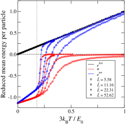
Figure 1: (Color online): Kinetic energy $e^{\mathrm{kin}}$, potential energy $u$, and total energy $e^{\mathrm{tot}}$ of a $3d$ system with $N=9$ particles as function of temperature $T$ for different system sizes $\tilde{L}$, as obtained from the molecular dynamics simulation. The transition temperature $T_{\mathrm{c}}$ is shown as dotted line.

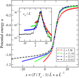
Figure 2: (Color online): Finite-size scaling plot of the potential energy $u$ and specific heat $c_{V}$ (inset) as function of the scaling variable $x$.

In the following, we present results of canonical simulations at fixed volume $V$, particle number $N$, temperature $T$, and magnetic field $\vec{B}$. We restrict $N$ to rather small values below 50 particles in order to keep the statistical errors small. As we want to compare our results to experiments done in the gas phase [9, 11], we consider systems with very low particle densities and focus on the case $L\rightarrow\infty$ at fixed $N$. Figure 1 shows the reduced kinetic energy $e^{\mathrm{kin}}=\langle E^{\mathrm{kin}}\rangle/E_{0}N$, the reduced potential energy $u=\langle\mathcal{U}\rangle/E_{0}N$ and the reduced total energy $e^{\mathrm{tot}}=\langle E^{\mathrm{tot}}\rangle/E_{0}N$ versus reduced temperature for a system consisting of $N=9$ particles, with different linear size $\tilde{L}=L/\sigma$ in three dimensions. $N=9$ is just one particular choice, $N>9$ yields similar results but larger statistical errors. It can be seen that the potential energy $u$ develops a jump with growing system size $L$, which results in a jump in the total energy $e^{\mathrm{tot}}$, as the kinetic part is simply proportional to temperature in the canonical ensemble (see eq. (9)). The $L$-dependence of $u$ stems from the fact that in a finite simulation volume particles which leave the bound state, chain or ring, are reflected back towards the bound structure by the boundaries. Thus the bound state is more stable in small volumes than in large or even infinite volume. This effect broadens the width of the transition and shifts the effective transition temperature $T_{\mathrm{c}}(L)$ to higher temperatures for smaller $L$.

In order to determine the nature of the transition as well as the critical temperature $T_{\mathrm{c}}$, a finite-size scaling plot of the potential energy $u(T)$ is shown in fig. 2, together with the specific heat at constant volume and constant number of particles, $c_{V}=\partial u/\partial T|_{V,N}$. Using the scaling variable

$$x=\left(\frac{T}{T_{\mathrm{c}}}-1\right)\tilde{L}+\frac{a}{\tilde{L}},$$ (10)

a data collapse both in $u(T)$ and in $c_{V}(T)$ can be achieved, leading to an estimation for the critical temperature $T_{\mathrm{c}}$,

$$k_{\mathrm{B}}T_{\mathrm{c}}=6.0(6)\times 10^{-2}E_{\mathrm{0}}.$$ (11)

The constant $a$ describes corrections to scaling and has the value $a=25(3)$. The fact that no rescaling is necessary in $u$ shows that the transition is of first order.

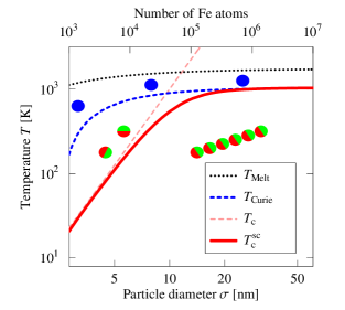
Figure 3: (Color online): Phase diagram of magnetic nanoparticles as function of particle size $\sigma$ and temperature $T$. Shown are the melting temperature (dotted black), the Curie temperature (dashed blue), and the chain building temperature, both with constant moment $\mu$ (long dashed pink) as well as with temperature dependent moment $\mu(T)$ (thick red), see text.

In the following discussion we neglect quantum mechanical effects which lead to, e.g., size-dependent magnetic moments in Fe particles with less than 1000 atoms [15]. In our model the ground state energy $E_{\mathrm{0}}$ depends on the size $\sigma$ and magnetic moment $\mu$ of the particle via eq. (3), leading to a simple dependence of the critical temperature $T_{\mathrm{c}}$ on the considered type of nanoparticles. For instance, Fe nanoparticles with a diameter of $\sigma\approx 6\,\textrm{nm}$ ($10^{4}$ atoms) have a saturation magnetization of $\mu\approx 2.2\times 10^{4}\mu_{\mathrm{B}}$, where $\mu_{\mathrm{B}}$ is the Bohr magneton. The critical temperature for the Fe nanoparticles follows from eq. (11) to $T_{\mathrm{c}}\approx 140\,\textrm{K}$. A resulting phase diagram for magnetic nanoparticles is depicted in fig. 3, where $T_{\mathrm{c}}(\sigma)$ is shown as a dashed line. As to lowest order, $T_{\mathrm{c}}(\sigma)\propto\sigma^{3}$, it has to be compared to other characteristic temperatures like the Curie temperature $T_{\mathrm{Curie}}$ and structural transition temperatures, e.g., the melting temperature $T_{\mathrm{Melt}}$, in order to determine the validity of the theory. Hence these two temperatures, which are size dependent as well, are also depicted schematically for typical magnetic systems. The finite-size form of $T_{\mathrm{Melt}}$ can be approximated to lowest order using energetic arguments to give $T_{\mathrm{Melt}}(\sigma)/T_{\mathrm{Melt}}^{\infty}=1-\sigma_{\mathrm{Melt}}/\sigma$ with material specific constant $\sigma_{\mathrm{Melt}}$ [16]. In the case of the magnetic transition, standard finite-size scaling theory gives, again to lowest order, a temperature shift of the form $T_{\mathrm{Curie}}(\sigma)/T_{\mathrm{Curie}}^{\infty}=1-(\sigma_{\mathrm{Curie}}/\sigma)^{1/\nu}$, with the exponent of magnetic correlations $\nu$ and constant $\sigma_{\mathrm{Curie}}$ [17]. As the magnetization $\mu$ vanishes at $T_{\mathrm{Curie}}$ as $\mu(T)=\mu(0)(1-T/T_{\mathrm{Curie}})^{\beta}$ with critical exponent $\beta$, and as $E_{0}$ is proportional to $\mu^{2}$ (eq. (3)), we can calculate a corrected $T_{\mathrm{c}}^{\mathrm{sc}}(\sigma)$ with temperature dependent magnetic moments as solution of the self-consistency equation

$$\frac{T_{\mathrm{c}}^{\mathrm{sc}}(\sigma)}{T_{\mathrm{c}}(\sigma)}=\left(1-\frac{T_{\mathrm{c}}^{\mathrm{sc}}(\sigma)}{T_{\mathrm{Curie}}(\sigma)}\right)^{2\beta},$$ (12)

shown in fig. 3 as thick red line [18]. For small particles $T_{\mathrm{c}}^{\mathrm{sc}}(\sigma)\approx T_{\mathrm{c}}(\sigma)$, as the rhs. of eq. (12) is approximately unity. On the other hand, for big particles $T_{\mathrm{c}}^{\mathrm{sc}}(\sigma)\approx T_{\mathrm{Curie}}(\sigma)$, as now the lhs. of eq. (12) is vanishing. As a result, in the case of Fe nanoparticles, a phase transition from ferromagnetic chains/rings to a ferromagnetic gas can occur for particle sizes below approximately 20 nm, while for larger particles the transition goes from ferromagnetic chains/rings to a paramagnetic gas.

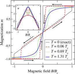
Figure 4: (Color online): Magnetization $m(B)$ of $N=25$ particles confined to a $2d$ surface as a function of the magnetic field $B$ for different temperatures $T$. The arrows indicate the direction of the hysteresis loop. The corresponding mean reduced potential energy $u(B)$ is shown in the inset.

In the following we consider two and three dimensional systems in an external magnetic field $\vec{B}$, which in the $2d$ case is oriented perpendicular to the plane. The field $B=|\vec{B}|$ allows us to analyze the stability of the structures which are observed in the simulations – namely a closed ring, a chain and a lattice-like structure in the $2d$ case. Typical hysteresis loops of a $2d$ system for different temperatures are shown in fig. 4. At low temperatures, $T=0.06~{}T_{\mathrm{c}}$, the system shows a broad hysteresis loop. Starting from the initial ring structure with the zero field value, $m=0$, the magnetization grows linearly while the moments of the particles start to turn into the direction of the increasing field. The following jump to the saturation value is related to the dissolving of the ring, because afterwards the particles are unbonded, forming a lattice-like structure on the $2d$ surface. Then, the moments of the particles point into the direction of the field, which gives rise to the saturation magnetization of the system. With decreasing field, the magnetization remains saturated and the particles stay in the lattice-like structure until this structure becomes unstable due to thermal fluctuations. The jump down to the linear part of the magnetization follows from the structural rearrangement of the particles back to the ring structure. With increasing temperature, the width of the hysteresis loop becomes smaller and vanishes at $T\approx 0.69~{}T_{\mathrm{c}}$. In the temperature range $0.69~{}T_{\mathrm{c}}\lesssim T<T_{\mathrm{c}}$ the potential energy $u(B)$ shows a cusp at $B_{\mathrm{c}}$ (see inset of fig. 4), which vanishes at the critical temperature $T_{\mathrm{c}}$. Above $T_{\mathrm{c}}$ the system is paramagnetic.

In the following, a simple model is presented, which, based on analytical ground state arguments like the potential energy, is able to explain qualitatively the numerical results in both $2d$ and $3d$ systems. For a large number of particles, $N\rightarrow\infty$, both the ring and the chain structures can be treated equally regarding their potential energy $u$. Due to the long-range nature of the dipolar interaction, the corresponding result for the reduced potential energy in the ground state is $u=-\zeta(3)$, where $\zeta(s)$ denotes the Riemann Zeta function. In both $2d$ and $3d$ systems at $T<T_{\mathrm{c}}$ and $B=0$ the particles form a ring, which is the most favorable state for $N\geq 4$ [19]. In the presence of a magnetic field oriented perpendicular to the system in $2d$, the equilibrium state is changed: In the $3d$ case, the ring plane turns perpendicular to the field, similar to the behavior of an antiferromagnetic spin systems in an external magnetic field. Furthermore, in both cases the magnetic moment $\vec{\mu}_{i}$ of each particle turns into the field direction by an angle $\alpha(B)$, leading to a potential energy per particle,

$$u(\alpha)=-\zeta(3)\left[\frac{3}{2}\cos^{2}(\alpha)-\frac{1}{2}+\sqrt{6}\frac{B}{B_{\mathrm{c}}}\sin(\alpha)\right]$$ (13)

with $B_{\mathrm{c}}=\sqrt{6}\zeta(3)E_{0}/\mu$. The equilibrium state is characterized by the angle

$$\alpha(B)=\arcsin\left(\sqrt{\frac{2}{3}}\frac{B}{B_{\mathrm{c}}}\right),$$ (14)

which follows from eq. (13) by requiring $\partial u/\partial\alpha=0$. Using this dependency, we can express the potential energy $u$ as a function of the magnetic field to get

$$u(B)=-\zeta(3)\left[1+\left(\frac{B}{B_{\mathrm{c}}}\right)^{2}\right].$$ (15)

This curve is shown as thin black line in the inset of fig. 4.

The ring structure remains stable as long as $B<B_{\mathrm{c}}$ and the dipolar interaction is attractive. This changes at $B=B_{\mathrm{c}}$, where the angle $\alpha$ approaches the critical value $\alpha(B_{\mathrm{c}})=\arcsin(\sqrt{2/3})\approx 54.74^{\circ}$. Here, the dipolar interaction becomes repulsive, leading to a break up of the ring due to the mobility of the particles (note that $B_{\mathrm{c}}$ is independent of the size of the particles; for saturated Fe spheres we find $B_{\mathrm{c}}\approx 0.47~{}\mathrm{T}$). In the $3d$ case, the particles rearrange in chains aligned parallel to the field, which is not possible in the $2d$ case, as the particles are confined to the surface. Instead, they rearrange in a hexagonal lattice-like structure on the surface, which is stabilized due to the repulsive character of the dipolar interaction. Now, both in three and in two dimensions, $u$ is mainly dominated by the field energy being proportional to $-B$ (see inset in fig. 4).

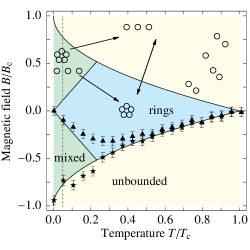
Figure 5: (Color online) Phase diagram of the $2d$ system. The arrows indicate the different structures of nanoparticles when crossing the phase boundaries. Stars mark the transition from the bonded to the unbonded phase, triangles the reverse transitions, as obtained from the molecular dynamics simulation. For clarity, the simulation data is only shown in the lower half plane. The dashed line marks the transition to the lattice-like structure with decreasing temperature.

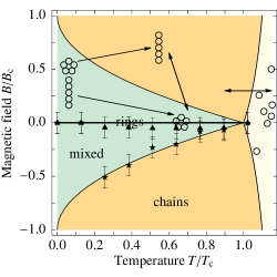
Figure 6: (Color online) Phase diagram of the $3d$ system. The arrows indicate the different structures of nanoparticles when crossing the phase boundaries. Stars mark the transition from the ring to the chain phase, triangles the reverse transitions, as obtained from the molecular dynamics simulation. For clarity, the simulation data is only shown in the lower half plane.

The reduced magnetization $m$ parallel to the magnetic field can be calculated for ring structures as a function of the field $B$, which yields

$$m(\alpha) = \frac{M(\alpha)}{M_{\mathrm{s}}}=\sin(\alpha),$$ (16)

$$m(B) = \sqrt{\frac{2}{3}}\frac{B}{B_{c}},$$ (17)

where $M_{\mathrm{s}}$ is the saturation magnetization (thin black line in fig. 4).

These ground state arguments can be expanded to describe the influence of temperature on the system, by specifying the transitions between the different states by purely energetic arguments. At finite temperatures and non-vanishing magnetic fields, the ring can be broken up by overcoming an energy barrier $\Delta u$ by thermal activation. This energy barrier separates the ring and the lattice-like structure in $2d$ and the ring and the chain structure in $3d$ respectively. Basically the barrier height is given by $\Delta u(B)=u(B_{\mathrm{c}})-u(B)$, which is the energy difference between the unstable ring and ring in equilibrium in the presence of the field $B$, (eq. (13)). If the mean kinetic energy equals this barrier height, the ring becomes unstable and dissolves. This and the equivalent consideration for the transition back to the ring structure leads to

$$B^{\uparrow}_{\mathrm{c}}(T)=B_{\mathrm{c}}\left(1-\sqrt{\frac{T}{T_{\mathrm{c}}}}\right).$$ (18)

If the field exceeds the critical value $B^{\uparrow}_{\mathrm{c}}(T)$, the ring dissolves into the lattice-like structure due to the kinetic fluctuations and the influence of the field. For fields lower than

$$B^{\downarrow}_{\mathrm{c}}(T)=B_{\mathrm{c}}\left(1+\sqrt{\frac{3}{2}}\right)\frac{T}{T}_{\mathrm{c}},$$ (19)

the dipolar particles flip back to the ring structure. Figure 5 shows the phase diagram of the $2d$ system using the calculated phase boundaries, eq. (18) and eq. (19), together with the data obtained from the molecular dynamics simulations. Both the lattice-like and ring structure can coexist in the area which is limited by these phase boundaries until the intersection is reached. If the temperature exceeds this boundary, only one state can survive depending on the field, leading to the loss of hysteresis. The pure ring phase is limited by the phase boundaries until $T_{\mathrm{c}}$ is reached. If the critical temperature $T_{\mathrm{c}}$ is reached at zero field, the rings dissolve and the particles enter the paramagnetic phase. For fields larger than $B^{\uparrow}_{\mathrm{c}}(T)$, the particles are unbonded, whereas the lattice-like structure is sustainable only at low temperatures, $T\ll T_{\mathrm{c}}$. The lattice-like structure gets lost due to the growing kinetic energy of the particles with increasing temperature.

The phase diagram of the $3d$ system is depicted in fig. 6. We find the pure chain phase and a mixed phase where both rings and chains can coexist. The pure ring phase is, in contrast to the $2d$ system, limited to $B=0$. Therefore, the area in which we can observe hysteresis is larger than in $2d$ systems. At high temperatures, $T>T_{\mathrm{c}}$, the system enters the paramagnetic phase, where the particles are unbonded. However, if the field is switched on the chain phase is again stabilized, because all particles are forced to point into the same direction. This makes an arrangement parallel to the field more favorable. At low temperatures, $T<T_{\mathrm{c}}$, and high fields, $B>B^{\uparrow}_{\mathrm{c}}$, the particles can arrange only in chains. If the field drops to zero, the chain closes to rings provided that this bending is affordable. Otherwise, a short chain will turn into the direction of the field without closing to a ring. In this case, the system can go from the upper to the lower mixed phase without entering the pure ring phase. This behavior depends on the length of the chain because it is more favorable to bend longer chains to closed rings than shorter ones. This shifts the starting point of the pure ring phase from $T=0$ to higher temperatures.

In this paper we have derived a phase diagram of dipolar nanoparticles as a function of particle size and temperature, explaining the transition from magnetic chains and rings to a magnetic gas. Furthermore, we have calculated the phase diagrams for two and three dimensional systems as a function of temperature and external magnetic fields by molecular dynamics simulations. The different regions of stability explain qualitatively the collective behavior of magnetic nanoparticles which has been observed in several experiments.

- [1] \BookSpringer Handbook of Nanotechnology \EditorBharat Bhushan \PublSpringer, Berlin \Year2006.
- [2] \BookAtomic clusters and nanoparticles. Agregats atomiques et nanoparticules: Les Houches Session LXXIII 2-28 July 2000 (Les Houches - Ecole d’Ete de Physique Theorique) \EditorC. Guet P. Hobza F. Spiegelmann F. David \Vol73 \PublSpringer, Berlin \Year2001.
- [3] \NameW. Wen, N. Wang, D. W. Zheng, C. Chen K. N. Tu J. Mater. Res. 14, 1186 (1998).
- [4] \NameA. Terheiden, O. Dmitrieva, M. Acet C. Mayer Chem. Phys. Lett. (2006), 431, 113-117.
- [5] \NameA. P. Hynninen M. Dijkstra Phys. Rev. Lett. 94, 138303 (2005).
- [6] \NameA.-P. Hynninen M. Dijkstra Phys. Rev. E 72, 051402 (2005).
- [7] \NameK. Butter, P. Bomans, P. M. Frederik, G. J. Vroege A. P. Philipse J. Phys: Condens. Matter 15, 1451 (2003).
- [8] \NameD. L. Blair A. Kudrolli Phys. Rev. E 67, 021302 (2003).
- [9] \NameJ. Knipping, H. Wiggers, B. F. Kock, T. Huelser, B. Rellinghaus P. Roth Nanotechnology 15, 1665 (2004).
- [10] \NameA. Snezhko, I. S. Aranson W. K. Kwok Phys. Rev. Lett. 94, 108002 (2005).
- [11] \NameT. Huelser, H. Wiggers, P. Ifeacho, O. Dmitrieva, G. Dumpich A. Lorke Nanotechnology 17, 3111 (2006).
- [12] \NameV. Salgueiriño-Maceira, M. A. Correa-Duarte, A. Hucht M. Farle J. Magn. Magn. Mater. 303, 163 (2006).
- [13] \NameL. Verlet Phys. Rev. 159, 98 (1967).
- [14] \NameH. C. Andersen J. Chem. Phys. 72, 2384 (1979).
- [15] \NameI. M. L. Billas, J. A. Becker, A. Châtelain, W. A. de Heer Phys. Rev. Lett. 71, 4067 (1993).
- [16] \NameP. Pawlow Z. Phys. Chem. 65, 1 (1909).
- [17] \NameP. V. Hendriksen S. Linderoth P.-A. Lindgard Phys. Rev. B 48, 7259 (1993).
- [18] In fig. 3 the following parameters are used: , , , , , and .
- [19] \NameW. Wen, F. Kun, K. F. Pal, D. W. Zheng K. N. Tu Phys. Rev. E 59, 4758 (1999).