Measuring the Expansion of the Universe Through Changes in the CMB Photosphere

Abstract

The expansion of the universe may be observed in “realtime” by measuring changes in the patterns of the anisotropy in the CMB. As the universe ages, the surface of decoupling—or the CMB photosphere—moves away from us and samples a different gravitational landscape. The response of the CMB to this new landscape results in a different pattern than we observe today. The largest change occurs at $\ell\approx 900$. We show that with an array of detectors that we may envision having in a couple of decades, one can in principle measure the change in the anisotropy with two high precision measurements separated by a century.

1. Introduction

Measurements of the anisotropy of the cosmic microwave background (CMB) provide a snapshot of the universe some 380,000 years after the big bang, when the primordial plasma decouples from the baryons. The power spectrum of the anisotropy is computed with a line of sight integration of the coupled Boltzmann equations between now and some time well before decoupling Seljak & Zaldarriaga (1996) (hereafter paper 1). This formalism may be extended to consider future times when the decoupling surface is further away from us. We may think of this as investigating an expanding CMB photosphere. Of course we do not know the details of the gravitational landscape beyond the current photosphere and so we can only probe the future in a statistical sense.

The conformal time of the decoupling surface in a flat universe is obtained from the Friedmann equation as follows:

$$\tau(a)=\int_{0}^{a}\frac{da^{\prime}}{H_{0}\sqrt{\Omega_{r,0}+a^{\prime}\Omega_{m,0}+a^{\prime 4}\Omega_{\Lambda,0}}},$$ (1)

where $a$ is the scale factor, $H_{0}$ is the current Hubble parameter, $\Omega_{r,0}$ is the current radiation density relative to the critical density, $\Omega_{m,0}$ is the current matter density relative to the critical density, and $\Omega_{\Lambda,0}$ is the current dark energy density relative to the critical density. At all times $\Omega_{r}+\Omega_{m}+\Omega_{\Lambda}=1$. With parameters inspired by the Wilkinson Microwave Anisotropy Probe (WMAP) Spergel et al. (2007), we take $\Omega_{r}=8.056\times 10^{-5}$, $\Omega_{m}=0.257$, $\Omega_{\Lambda}=0.743$ and $H_{0}=72~{}{\rm km/s/Mpc}$. The current conformal distance to the decoupling surface ($a=1$ in the above equation) is $c\tau=14373$ Mpc.

Table 1Time slices and Scale Factors

Time slice	$c\tau$	Scale factor
Years	Mpc	$a$
0	14373	1.0000
$1\times 10^{8}$	14403	1.0074
$5\times 10^{8}$	14523	1.0372
$1\times 10^{9}$	14669	1.0754
$2\times 10^{9}$	14944	1.1545
$4\times 10^{9}$	15440	1.3255
$5\times 10^{9}$	15663	1.4182
$6\times 10^{9}$	15872	1.5163
$8\times 10^{9}$	16251	1.7304
$1\times 10^{10}$	16583	1.9714
$4\times 10^{10}$	18657	13.340
$1\times 10^{11}$	19011	601.95

Note. — To find the physical time of any time slice add $13.66\times 10^{9}$ years, the current age of the universe for our adopted parameters. Because $d\tau=dt/a$, the physical time is computed from equation 1 except with an additional factor of $1/a^{\prime}$ in the integrand. Note that the universe doubles in diameter when the physical time is 75% greater than today and the conformal time is 15% greater.

2. Computing the Power Spectrum

To perform our study, we use CAMB Lewis et al. (2000) which follows the algorithm in Seljak and Zaldarriga’s CMBFAST Seljak & Zaldarriaga (1996). We consider only scalar perturbations. We modified the CAMB code so that it computes the following evolution function (eq. 13 in paper 1)

$$\Delta_{T_{\ell}}(\tau_{f},k)=\int_{0}^{\tau_{f}}S(\tau,k)j_{\ell}\left[k(\tau_{f}-\tau)\right]d\tau$$ (2)

where $S$ is the source function, $j_{\ell}$ is a spherical Bessel function, $\tau$ is the conformal time, and $k$ is the comoving wavevector of the perturbation. The modification allows for arbitrary final $\tau$ (as opposed to fixing $\tau_{f}=\tau_{0}$). The source function is given by

$$S(k,\tau)=e^{\kappa_{f}}\left[g\left(\Delta_{T_{0}}+\Psi\right)+\frac{\partial}{\partial\tau}\left(g\frac{v_{b}}{k}\right)+e^{-\kappa}\left(\dot{\Phi}+\dot{\Psi}\right)+P(k,\tau)\right]$$ (3)

where $P(k,\tau)$ represents polarization terms (see eq. 12 in paper 1) which we ignore for simplicity. Here $g(\tau)=-\dot{\kappa}e^{-\kappa}$ is the visibility function with $\kappa(\tau)$ the optical depth from $\tau_{0}$ (note that for $\tau_{f}>\tau_{0}$, $\kappa_{f}<0$). Eq. (3) differs from eq. 12 in paper 1 only in the overall $e^{\kappa_{f}}$ term which accounts for the changing optical depth. The first order term in the expansion of the Boltzmann equation, $\Delta_{T0}$ (eq. 3a in paper 1), the potentials $\Psi$ and $\Phi$, the velocity of the baryons $v_{b}$, and the polarization terms are computed by CAMB and need no modification. The primary modification to CAMB is to calculate $S$ out to $\tau_{f}$, rather than to $\tau_{0}$. In addition, some of CAMB’s optimizations that led to sparse sampling at recent times were removed.

To compute the power spectrum at any time in the future we simply form the analog of eq 9 in paper 1:

$$C_{\ell}(\tau_{f})=(4\pi)^{2}\int k^{2}P_{\Psi}(k)\left[\Delta_{T_{\ell}}(0,\tau_{f},k)\Delta_{T_{\ell}}^{*}(0,\tau_{f},k)\right]dk$$ (4)

where $P_{\Psi}(k)$ is the initial power spectrum. Figure 1 shows the power spectrum for future times. We see three major effects: (1) The power spectrum amplitude drops off due to the $1/a$ scaling of the CMB temperature; (2) The features shift to smaller angular scales due to the recession of the surface of last scattering; (3) The low-$\ell$ tail becomes enhanced compared to the peak due to the integrated Sachs-Wolfe (ISW) effect caused by the shift to dark-energy dominance. The enhanced ISW effect is not present in runs of the code without dark energy. In roughly $25\times 10^{9}$ years, the ISW effect at $\ell=2$ will exceed the height of the first acoustic peak.

Figure 1.— The temperature angular power spectrum of the CMB at several representative time steps into the future. The scale factors and conformal distances are given in Table 1. The shift to the right of the first acoustic peak for some future time is $\ell_{f}=\ell_{0}(\tau_{f}-\tau_{dec})/(\tau_{0}-\tau_{dec})$ where $\tau_{dec}=286~{}{\rm Mpc}$ is the conformal time of decoupling, and $\ell_{0}=220$ the current $\ell$ of the acoustic peak.

3. Maps of the future sky

To visualize the evolution of the CMB photosphere, we make maps of the sky for various physical time slices (see Table 1). For any particular map, which we take as a Gaussian random field, all the information is contained in the power spectrum, $C_{\ell}=<a_{\ell m}a^{\star}_{\ell m}>$, where the $a_{\ell m}s$ are the coefficients of a spherical harmonic decomposition of the map. To generate a visualization, one draws $\ell+1$ random normal complex deviates, r, with variance $C_{\ell}$ to generate a set of $2\ell+1$ $a_{\ell m}$s that satisfy $a_{\ell-m}=a_{\ell m}^{\star}$. From these one forms the real valued $T(\theta,\phi)=\sum_{\ell m}a_{\ell m}Y_{\ell m}(\theta,\phi)$.

A set of maps that shows the future evolution of the CMB will be correlated. To account for this, we compute the full covariance matrix

$$C_{\ell}^{ij}=(4\pi)^{2}\int k^{2}P_{\Psi}(k)\left[\Delta_{T_{\ell}}(0,\tau^{i},k)\Delta_{T_{\ell}}^{*}(0,\tau^{j},k)\right]dk,$$ (5)

where $\tau^{i}$ is the conformal time at any time in the future. Thus for a sequence of say $n$ maps, we would compute a $n\times n$ matrix for each $\ell$.

We now extend the method given above to generate a set of correlated $a_{lm}$s. The first step is to decompose the covariance matrix as ${\mathbf{C}}_{\ell}={\mathbf{M}}_{\ell}{\mathbf{D}}_{\ell}{\mathbf{M}}_{\ell}^{\star}$ where ${\mathbf{D}}_{\ell}$ is a diagonal matrix. We then compute ${\mathbf{a}}_{\ell m}={\mathbf{M}}_{\ell}[\sqrt{{\mathbf{D}}_{\ell}}]{\mathbf{r}}$ where ${\mathbf{r}}$ is a vector of complex random deviates. This $\mathbf{a}_{\ell m}$ has the covariance matrix in eq. 5. Figures 2-5 show a set of four time slices starting with a random full-sky map that follows the WMAP parameters. One can see that most of the change occurs on small angular scales where the photosphere more quickly samples different potential wells as it expands. One also sees that as time progresses large angular scale fluctuations become more prominent as dark energy dominates the expansion.

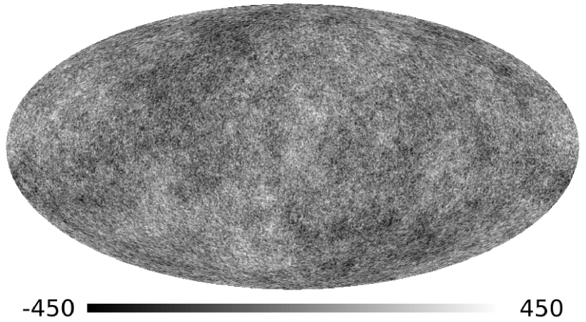
Figure 2.— Present map for a set of random variables that follows the WMAP power spectrum. The units on the color bar are ${\rm\mu K}$.

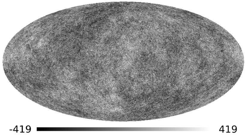
Figure 3.— The same map as in Figure 2 but now for a time slice $1\times 10^{9}$ years in the future. Note that the color bar has been rescaled. The primary difference between the two maps is at small angular scales.

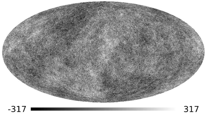
Figure 4.— The same map as in Figure 2 but now for a time slice $5\times 10^{9}$ years in the future. Again, the color bar has been rescaled.

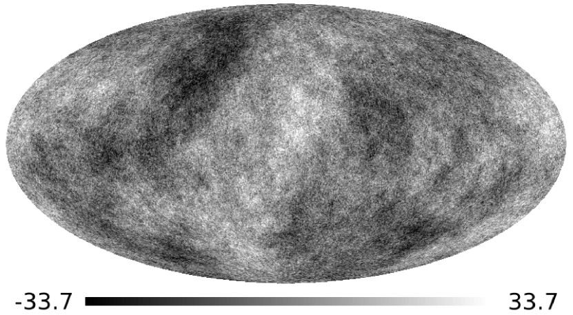
Figure 5.— The same map as in Figure 2 but now for a time slice $40\times 10^{9}$ years in the future. The color bar has been rescaled. Note that the large angular scale fluctuations are more prominent relative to the smaller angular scales.

Figure 6 shows elements of the covariance matrix as a function of time. As expected, nearby time slices are strongly correlated. As time progresses the covariance between current and future time slices at small angular scales disappears first, and then later the covariance at large angles decreases. The time it takes for the scale factor to double, $\approx 10^{10}$y, gives a characteristic time for the future sky to decorrelate with what we observe today.

Figure 7 gives the correlation of several time steps with the present. In this plot, the decrease in temperature has been scaled out so that features in the anisotropy may be compared directly. At high $\ell$, features in the sky at late times are uncorrelated with those at present. However, at low $\ell$, the late-time ISW features remain correlated for $>100$ billion years, indicating that these are very long lived structures.

Figure 6.— The $C_{\ell}^{0j}$ element of the covariance matrix for several time slices. The power spectrum at $\tau_{0}$ is also plotted for comparison. Some of the decrease in the covariance is attributable to the decrease in the CMB temperature. For example, in $10^{9}$ years the power at $\ell=200$ decreases to 36% the current value but 16% of the decrease arrises because $T=T_{0}/a$.

Figure 7.— The correlation of several time slices with the present.

4. Measuring the Change in the CMB

Measuring the difference between two high precision maps of the anisotropy taken a century apart offers, in principle, a way to directly observe the expansion of the universe. Unlike a measurement of the temperature of the CMB, the difference between two maps is moderately insensitive to calibration. Rather, it is a change in spatial structure that is observed. Thus one needs a well understood pointing solution which is technically straightforward to achieve.

Figure 8 shows the power spectrum of the difference between two maps taken 100 years apart. We use the formalism in Knox (1995) to compute the experimental uncertainty. Since there is just one sky realization, cosmic variance is ignored and the uncertainty per $\ell$ is

$$\Delta C_{\ell}=\sqrt{\frac{2}{f_{sky}(2\ell+1)}}\sigma^{2}\Omega_{pix}\exp(\ell^{2}\theta_{1/2}^{2}/8\ln 2),$$ (6)

where $f_{sky}$ is the fraction of sky covered, $\sigma$ is the uncertainty per sky pixel of solid angle $\Omega_{pix}$, and $\theta_{1/2}$ is the FWHM of the beam profile. For the uncertainty bands shown in Figure 8, we imagine an array of 3000x3000 detectors at 150 GHz each with a sensitivity of 40 mK s^1/2 Bock et al. (2006) observing the sky with $0.86^{\prime}$ angular resolution. The observations would last 4 years, cover 75% of the sky, and would have to be done from a satellite. The only element not already demonstrated is large array. Currently, arrays of 32x32 detectors are being built.

Figure 8.— The top curves shows the current CMB EE polarization spectrum for the parameters in this paper and a current optical depth of 0.1. The two curves below that show the BB spectrum for tensor to scalar ratios of $r=0.3$ and $r=0.01$. The solid curve at the bottom is the power spectrum of the difference between two CMB anisotropy maps made 100 years apart. The dotted line is Equation 6 and the hashed boxes show the errors after binning in $\ell$.

The fundamental limit to such a measurement is likely to be variable point sources and variable foreground emission. Though in principle these can be identified and removed spectrally, this capability would add complexity to the “simple” scheme outlined above. For comparison, there are currently experiments being designed with the sensitivity to measure the $r=0.01$ B-mode polarization. The improvement to go from these planned missions to measuring the signal we describe is on the order of the improvement between observations of the 1980s and the current observations.

References

- Bock et al. (2006) Bock, J. et al., “Task Force on Cosmic Microwave Background Research,” also known as “The Weiss Report,” astro-ph/0604101, 2006.
- Górski et al. (1999) Górski, K., Hivon, E., Wandelt, B. in Proceedings of the MPA/ESO Cosmology Conference “Evolution of Large-Scale Structure”, eds. A.J. Banday, R.S. Sheth, and L. Da Costa, PrintPartners Ipskamp, NL, pp. 37-42. 1999. The HEALPix code is available at http://healpix.jpl.nasa.gov/.
- Knox (1995) Knox, L., Phys.Rev. D52:4307, 1995.
- Lange (2007) Lange, S., “The Time Evolution of the Cosmic Microwave Background Photosphere,” Senior thesis in the Dept. of Physics, Princeton University, 2007.
- Lewis et al. (2000) Lewis, A., Challinor, A., & Lasenby, A., ApJ, 538:473, 2000. The CAMB code is available at http://camb.info/.
- Seljak & Zaldarriaga (1996) Seljak, U. & Zaldariagga, M., ApJ, 468:437, 1996.
- Spergel et al. (2007) Spergel et al. ApJS, 170:377, astro-ph/0603449, 2007.