Hall Transport in Granular Metals and Effects of Coulomb Interactions

Abstract

We present a theory of Hall effect in granular systems at large tunneling conductance $g_{T}\gg 1$. Hall transport is essentially determined by the intragrain electron dynamics, which, as we find using the Kubo formula and diagrammatic technique, can be described by nonzero diffusion modes inside the grains. We show that in the absence of Coulomb interaction the Hall resistivity $\rho_{xy}$ depends neither on the tunneling conductance nor on the intragrain disorder and is given by the classical formula $\rho_{xy}=H/(n^{*}ec)$, where $n^{*}$ differs from the carrier density $n$ inside the grains by a numerical coefficient determined by the shape of the grains and type of granular lattice. Further, we study the effects of Coulomb interactions by calculating first-order in $1/g_{T}$ corrections and find that (i) in a wide range of temperatures $T\gtrsim\Gamma$ exceeding the tunneling escape rate $\Gamma$, the Hall resistivity $\rho_{xy}$ and conductivity $\sigma_{xy}$ acquire logarithmic in $T$ corrections, which are of local origin and absent in homogeneously disordered metals; (ii) large-scale “Altshuler-Aronov” correction to $\sigma_{xy}$, relevant at $T\ll\Gamma$, vanishes in agreement with the theory of homogeneously disordered metals.

I Introduction

Hall transport in different systems has always been a subject of extensive research. Already the classical Drude-Boltzmann theory provides us with an interesting result. It is well-known that the Hall resistivity (HR)

$$\rho_{xy}=\frac{H}{nec}$$ (1)

of a disordered metal does not depend on the mean free path and is determined solely by the carrier concentration $n$ allowing one to extract it experimentally. At low enough temperatures quantum effects of Coulomb interaction and weak localization (see, e.g., Refs. AA, ; LR, ) influence the Hall transport, giving corrections to Eq. (1).

Dense-packed arrays of metallic or semiconducting nanoparticles imbedded into an insulating matrix, usually called granular systems or nanocrystals, have recently received much attention from both experimental and theoretical sides (see a Review BELVreview, and references therein). The longitudinal transport in such systems is theoretically well understood now, both in the metallic and insulating regimes. At the same time, Hall transport in such granular materials has not been addressed theoretically before, neither in the insulating nor in the metallic regimes. The absence of a theoretical description is apparently one of the reasons, why measurements of the Hall resistivity have not become a standard tool for characterization of granular metals, although they do not seem to be very difficult.

Trying to apply the conventional theory of disordered metals to granular systems, the following questions can be asked: To what extent is the formula (1) applicable to granular metals? How is the carrier concentration extracted from Eq. (1) related to the actual carrier concentration inside the grains? What impact do quantum effects have on Hall transport of a granular system?

In this paper we present a theory of Hall effect in a granular system in the metallic regime and answer these questions.

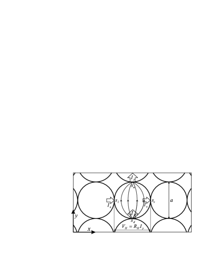
Figure 1: Granular system and classical picture of Hall conductivity. The external Ohmic voltage $V_{y}$ is applied to the contacts in the $y$ direction. The resulting Ohmic current $I_{y}=G_{T}V_{y}$ running through the grain in the $y$ direction causes the Hall voltage drop $V_{H}=R_{H}I_{y}$ between its opposite banks in the $x$ direction. Since for calculating Hall conductivity $\sigma_{xy}$ the total voltage drop per lattice period in the $x$ direction is assumed 0, the Hall voltage $V_{H}$ is also applied (with an opposite sign) to the contacts in the $x$ direction, causing the Hall current $I_{x}=G_{T}V_{H}=G_{T}^{2}R_{H}V_{y}$ [Eq. (5)].

In the metallic regime (“granular metal”), when the intergrain tunneling conductance $G_{T}=(2e^{2}/\hbar)g_{T}$ is large, $g_{T}\gg 1$ (further we set $\hbar=1$), the granular system as a whole is, roughly speaking, a good conductor and its properties are quite similar to those of ordinary homogeneously disordered metals (HDMs). At the same time the granularity of the system brings a new physical aspect: confinement of electrons inside the grains. In a system with “well-pronounced” granularity electron traverses each grain many times before it escapes from it to some neighboring grain due to tunneling. This is ensured by the condition that the tunneling escape rate $\Gamma$ is much smaller than the Thouless energy $E_{\text{Th}}$ of the grain:

$$\Gamma\ll E_{\text{Th}},$$ (2)

or, equivalently, the tunneling conductance $G_{T}$ is much smaller than the longitudinal conductance $G_{0}=(2e^{2}/\hbar)g_{0}$ of the grain:

$$g_{T}\ll g_{0},$$ (3)

since $\Gamma=g_{T}\delta$ and $E_{\text{Th}}\propto g_{0}\delta$ ($\delta$ is the mean level spacing of the grain).

The conditions (2) and (3), leading to new physicsBELVreview absent in HDMs, simplify calculations at the same time. Consider, for example, the classical (in the absence of quantum effects, such as Coulomb interaction and weak localization) longitudinal conductivity (LC) $\sigma_{xx}^{(0)}$ of a regular quadratic or cubic granular lattice (Fig. 1) with all contacts having equal conductances $G_{T}$. In the limit $g_{T}\ll g_{0}$ the main contribution to the longitudinal resistivity (LR) $\rho_{xx}^{(0)}=1/\sigma_{xx}^{(0)}$ comes from the tunnel barriers between the grains rather than from scattering on impurities inside the grains and LC equals

$$\sigma^{(0)}_{xx}=G_{T}a^{2-d},$$ (4)

where $a$ is the size of the grains and $d=2,3$ is the dimensionality of the array. The longitudinal conductance $G_{0}$ of the grain itself, which, in principle, should be obtained from a solution of a classical electrodynamics problem for the distribution of the electric potential inside the grain and is, therefore, determined by the properties of the intragrain electron dynamics, does not enter Eq. (4).

Thus, when studying longitudinal transport one may neglect the details of electron dynamics inside the grains, which is a significant simplification. Technically, this is equivalent to considering only the zero (coordinate-independent inside the grains) spatial modes of the diffusons or phases in the phase functionalET ; BELVreview . Owing to the conditions (2) and (3), the zero-mode approximation suffices for studying the longitudinal transport.

For Hall transport, however, the situation appears to be more complicated. The Hall current originates from the transversal drift in the crossed magnetic and electric fields inside the grains. The classically prohibited regions of tunnel contacts are neglegibly small for dense-packed arrays and cannot contribute to the Hall transport. From simple classical considerations (see Fig. 1) one obtains, that Hall conductivity (HC) $\sigma_{xy}^{(0)}$ in the leading in $g_{T}/g_{0}\ll 1$ order is

$$\sigma^{(0)}_{xy}=G_{T}^{2}R_{H}a^{2-d},$$ (5)

where $R_{H}$ is the Hall resistance of the grain. Just like $G_{0}$, the Hall resistance $R_{H}$ should be obtained from a solution of a classical electrodynamics problem for the distribution of the electric potential inside the grain. We come to the situation when one is forced to take the intragrain electron dynamics into account, no matter how well the conditions (2) and (3) are satisfied. In other words, the zero-mode approximation is not sufficient for the description of the Hall transport of a granular system.

However, a purely classical approach to the problem, giving a quick answer (5), does not allow one to include quantum effects (such as Coulomb interaction and weak localization) into considerations, which come into play at sufficiently low temperatures and can significantly affect transport properties.

In this work we develop a method of calculating conductivity of a granular system in the metallic regime, which allows one to take the intragrain electron dynamics into account. Using the Kubo formula and diagrammatic technique, we show that this can be done by considering nonzero (coordinate-dependent) modes of standard two-particle propagators (“diffusons”) inside the grains. This procedures accounts for the finiteness of the ratio $g_{T}/g_{0}$ and reproduces the solution of the classical electrodynamics problem for the conductivity of a granular medium. The generality of our approach allows one, in principle, to study both LC and HC of the granular system for arbitrary ratio $g_{T}/g_{0}$ and for arbitrary type of the intragrain electron dynamics, either ballistic or diffusive. Nonzero modes of the diffusons are eventually related to the longitudinal $G_{0}^{-1}$ and Hall $R_{H}$ resistances of the grain.

We apply our method to the problem of Hall transport, for which considering intragrain dynamics is inevitable. Neglecting quantum effects, we do recover the classical formula (5) for the Hall conductivity and obtain quite a universal result for the Hall resistivity. Diagrammatic approach allows us to include quantum effects of Coulomb interaction and weak localization straightforwardly into the developed scheme. We study the influence of Coulomb interactions on HC and HR by calculating first-order corrections and find that the major temperature dependence of both HC and HR of a granular metal comes from the contributions which are absent in HDMs. We also announce our results for weak localization corrections, detailed calculations of which will be presented elsewhere KEprepWL . Part of the results of our work (for temperatures $T\gtrsim\Gamma$) was presented in a brief form in Ref. KEletter, .

The paper is organized as follows. In Sec. II we present our results for Hall conductivity and resistivity and Coulomb interaction corrections to them. In Sec. III the model for the granular system is formulated and discussed. In Sec. IV the main features of the diagrammatic technique are explained, and important building blocks, namely, the intragrain diffuson in the presence of magnetic field and the screened Coulomb interaction, are obtained. In Sec. V we calculate Hall conductivity neglecting quantum effects of Coulomb interaction and obtain the correspondence with the classical result. Quantum effects of Coulomb interaction are studied in Sec. VI. Concluding remarks are presented in Sec. VII. In Appendix A the boundary condition for the intragrain diffuson in the presence of magnetic field is derived.

II Results

In this section we list the main results of this work. We perform calculations for magnetic fields $H$ such that $\omega_{H}\tau_{0}\ll 1$, where $\omega_{H}=eH/(mc)$ is the cyclotron frequency and $\tau_{0}$ is the electron scattering time inside the grain. Since the (effective) electron mean free path $l=v_{F}\tau_{0}\lesssim a$ does not exceed the grain size $a$, and typically $a\approx 1-100\text{nm}$, the condition $\omega_{H}\tau_{0}\ll 1$ is well fulfilled even for experimentally high fields $H$. We also assume that the granularity of the system is “well-pronounced”, i.e., the conditions (2) and (3) are satisfied. Other assumptions and approximations are formulated in Sec. III.

Classical Hall conductivity and resistivity. First, we neglect quantum effects of Coulomb interaction and obtain Eq. (5) for HC $\sigma^{(0)}_{xy}$ in the lowest nonvanishing order in $g_{T}/g_{0}\ll 1$. This result obtained by diagrammatic methods is of completely classical origin provided the tunneling contacts are viewed as surface resistors with conductance $G_{T}$. The HR of the system

$$\rho^{(0)}_{xy}=\frac{\sigma^{(0)}_{xy}}{(\sigma^{(0)}_{xx})^{2}}=R_{H}a^{d-2}$$ (6)

following from Eqs. (4) and (5), thus, does not depend on the tunneling conductance $G_{T}$ and is expressed solely through the Hall resistance $R_{H}$ of a single grain. Further, the Hall resistance $R_{H}$ of the grain does not depend on the intragrain disorder, but only on the geometry of the grain and carrier density $n$ of the grain material. For grains of a simple geometry (e.g., having reflectional symmetry in all three dimensions) $R_{H}=\rho_{xy}^{\text{gr}}a/S$ , where $\rho_{xy}^{\text{gr}}=H/(nec)$ is the specific Hall resistivity of the grain material and $S$ is the area of the largest cross section of the grain.

Therefore, akin to the universal result (1) for ordinary disordered metals, for the classical Hall resistivity of a granular metal we obtain

$$\rho^{(0)}_{xy}=\frac{H}{n^{*}ec}$$ (7)

in the case of a three-dimensional sample (3D, $d=3$, many grain monolayers). Here,

$$n^{*}=An,\mbox{ }A=\frac{S}{a^{2}}\leq 1,$$

is the effective carrier density of the system, which differs from the actual carrier density $n$ inside the grains only by a numerical factor $A$ determined by the shape of the grains ($A=\pi/4$ for spherical and $A=1$ for cubic grains). For a two-dimensional sample (2D, $d=2$, one or a few grain monolayers) the expression (7) must divided by the thickness $d_{z}$ of the sample or, equivalently, $n^{*}=d_{z}An$ in this case.

The result (7) for the Hall resistivity $\rho^{(0)}_{xy}$ is quite universal. It is valid even if (i) the tunneling conductances $G_{T}$ fluctuate from contact to contact and (ii) the mean free path $l$ fluctuates from grain to grain: HR is simply independent of the distributions of $G_{T}$ and $l$; Therefore, Eq. (7) is applicable to real granular arrays in which such irregularities are always present (provided such system is still in the metallic regime). We also note that although Eq. (6) was obtained for a regular quadratic/cubic granular lattice, the result (7) with a different factor $A\leq 1$ remains valid for other regular lattices (e.g., more common for real experimental samples triangular lattice). We also expect Eq. (7) to hold for arrays with moderate structural disorder, i.e., in which the positions of the grains deviate from regular and their sizes and shapes are not identical.

Coulomb interaction corrections. Next, we calculate the first-order in $1/g_{T}$ corrections to HC $\sigma^{(0)}_{xy}$ [Eq. (5)] due to Coulomb interaction. We find significant contributions for temperatures $T\lesssim g_{T}E_{c}$ not exceeding the inverse $RC$ time $g_{T}E_{c}$ of the system “grain+contact” [$E_{c}=e^{2}/(\kappa a)$ is the charging energy and $\kappa$ is the dielectric constant of the array], whereas for $T\gtrsim g_{T}E_{c}$ the relative corrections are of the order of $1/g_{T}$ or smaller. Three types of corrections to HC $\sigma^{(0)}_{xy}$ [Eq. (5)] can be identified:

$$\sigma_{xy}=\sigma^{(0)}_{xy}+\delta\sigma_{xy}^{TA}+\delta\sigma_{xy}^{VD}+\delta\sigma_{xy}^{AA}.$$ (8)

The first correction $\delta\sigma_{xy}^{TA}$ can be attributed to the renormalization of the individual tunneling conductances $G_{T}$ [tunneling anomaly (TA) AA ; TA1 ; TA2 ] in the granular medium and has the form

$$\frac{\delta\sigma^{TA}_{xy}(T)}{\sigma^{(0)}_{xy}}=-\frac{1}{\pi g_{T}d}\ln\left[\frac{g_{T}E_{c}}{\max(T,\Gamma)}\right]\mbox{ for }T\lesssim g_{T}E_{c}.$$ (9)

This correction renormalizes the tunneling conductances $G_{T}$ in Eq. (5), but does not affect the Hall resistance $R_{H}$ of the grain.

The second correction $\delta\sigma_{xy}^{VD}$ corresponds to the process of virtual diffusion (VD) of electrons through the grain and equals

$$\frac{\delta\sigma^{VD}_{xy}(T)}{\sigma^{(0)}_{xy}}=\frac{c_{d}}{4\pi g_{T}}\ln\left[\frac{\min(g_{T}E_{c},E_{\text{Th}})}{\max(T,\Gamma)}\right]$$ (10)

for $T\lesssim\min(g_{T}E_{c},E_{\text{Th}})$, where $c_{d}\sim 1$ is a numerical lattice structure factor (101). Contrary to $\delta\sigma_{xy}^{TA}$, the correction $\delta\sigma_{xy}^{VD}$ is suppressed at temperatures greater than the Thouless energy of the grain $E_{\text{Th}}$, which emphasizes its diffusion character.

For $T\gtrsim\Gamma$ both corrections $\delta\sigma_{xy}^{TA}$ and $\delta\sigma_{xy}^{VD}$ are $\ln T$-dependent. This dependence saturates at temperatures $T\sim\Gamma$, so that $\delta\sigma_{xy}^{TA}$ and $\delta\sigma_{xy}^{VD}$ remain logarithmically large constants at $T\lesssim\Gamma$. These two corrections are specific for granular systems and, in essence, due to the strong discrepancy of timescales of the intra- ($E_{\text{Th}}^{-1}$) and intergrain ($\Gamma^{-1}$) electron dynamics described by Eq. (2). They arise from spatial scales of the order of the grain size $a$ and are absent in HDMs. The logarithmic behavior of the corrections (9) and (10) is due to the form of the screened Coulomb interaction in granular systemsBEAH . They have the same logarithmic form in 2D and 3D, but the coefficients are not universal and lattice-dependent: $1/d$ and $c_{d}$ [Eq. (101)] are the results for the cubic (3D) or quadratic (2D) lattice, which we assumed in our calculations.

The third correction $\delta\sigma_{xy}^{AA}$ in Eq. (8) is analogous to the one present in homogeneously disordered metalsAA [“Altshuler-Aronov” (AA) corrections]. It can be significant at low temperatures $T\ll\Gamma$ only, when the thermal length $L_{T}=\sqrt{D_{0}^{*}/T}\gg a$ for the intergrain motion exceeds the grain size $a$ ($D_{0}^{*}=\Gamma a^{2}$ is the effective diffusion coefficient for the intergrain electron motion at scales greater than $a$). However, we find that this correction vanishes identically both in 2D and 3D:

$$\delta\sigma_{xy}^{AA}=0.$$ (11)

It is always instructive to compare the results for a granular metal with those for a HDM. The quantities arising from large spatial scales (exceeding the grain size $a$ for a granular metal and the mean free path $l$ for a HDM) are expected to behave universally, because at such scales the microscopic structure of the system becomes irrelevant. Indeed, the result (11) for $\delta\sigma_{xy}^{AA}$ agrees with the one for HDMs first obtained in Ref. AKLL, . Being an exact cancellation, however, Eq. (11) is valid not only for low $T\ll\Gamma$, but for arbitrary relevant temperatures.

The quantity directly measured in experiments is the Hall resistivity

$$\rho_{xy}=\frac{\sigma_{xy}}{\sigma_{xx}^{2}}=\rho_{xy}^{(0)}+\delta\rho_{xy},$$ (12)

where $\rho_{xy}^{(0)}$ is the “bare” HR [Eq. (7)], $\delta\rho_{xy}$ is the total Coulomb interaction correction to HR and HC $\sigma_{xy}$ is given by Eq. (8). The interaction corrections to LC were studied in Refs. ET, ; BELV, and the following result was obtained:

$$\sigma_{xx}=\sigma^{(0)}_{xx}+\delta\sigma_{xx}^{TA}+\delta\sigma_{xx}^{AA}$$ (13)

[$\delta\sigma_{xx}^{TA}$ and $\delta\sigma_{xx}^{AA}$ correspond to $\delta\sigma_{1}$ [Eq. (2b)] and $\delta\sigma_{2}$ [Eq.(2c)] in Ref. BELV, , respectively]. The correction $\delta\sigma_{xx}^{TA}$ is due to the tunneling anomaly in granular metal. It renormalizes the tunneling conductance $G_{T}$ in Eq. (4) and equals

$$\frac{\delta\sigma^{TA}_{xx}(T)}{\sigma^{(0)}_{xx}}=-\frac{1}{2\pi g_{T}d}\ln\left[\frac{g_{T}E_{c}}{\max(T,\Gamma)}\right]\mbox{ for }T\lesssim g_{T}E_{c}.$$ (14)

This correction is of local origin and governs the temperature dependence of LC $\sigma_{xx}(T)$ in a wide temperature range. The Hall counterpart of $\delta\sigma_{xx}^{TA}$ is $\delta\sigma_{xy}^{TA}$ [Eq. (9)].

The correction $\delta\sigma_{xx}^{AA}$ is analogous to that in a HDM, first obtained by Altshuler and Aronov (AA) in Ref. AAjetp, and its Hall counterpart is $\delta\sigma_{xy}^{AA}$ [Eq. (11)]. The AA correction $\delta\sigma_{xx}^{AA}$ does not diverge at large spatial scales in 3D case, being smaller than the logarithmic contributions (9), (10), (14) for all relevant temperatures down to very low onesBELV : $\delta\sigma_{xx}^{AA}/\sigma_{xx}^{(0)}\lesssim 1/g_{T}$.

In 2D case, i.e. for granular films of thickness $d_{z}$ consisting of one or a few grain monolayers ($d_{z}/a$ is the number of monolayers), the correction $\delta\sigma_{xx}^{AA}$ is diverging at large spatial scales. This divergence is relevant for low temperatures $T\ll\Gamma(a/d_{z})^{2}$ (when $L_{T}^{*}\gg d_{z}$), for which $\delta\sigma_{xx}^{AA}$ acquires a logarithmic dependenceBELV :

$$\frac{\delta\sigma^{AA}_{xx}(T)}{\sigma^{(0)}_{xx}}=-\frac{1}{4\pi^{2}g_{T}}\ln\left[\frac{\Gamma}{T}\left(\frac{a}{d_{z}}\right)^{2}\right],$$ (15)

The total Coulomb interaction correction

$$\delta\rho_{xy}=\delta\rho_{xy}^{TA}+\delta\rho_{xy}^{VD}+\delta\rho_{xy}^{AA}$$ (16)

to Hall resistivity (12) is given by the sum of the contributions arising from the corresponding corrections to Hall (8) and longitudinal (13) conductivities as

$$\frac{\delta\rho_{xy}^{(i)}}{\rho_{xy}^{(0)}}=\frac{\delta\sigma_{xy}^{(i)}}{\sigma^{(0)}_{xy}}-2\frac{\delta\sigma_{xx}^{(i)}}{\sigma^{(0)}_{xx}},\mbox{ }(i)=TA,VD,AA.$$

Since the TA effects leads to the renormalization of the tunneling conductance $G_{T}$ only, it cannot affect the HR $\rho^{(0)}_{xy}$ [Eq. (7)], which does not contain $G_{T}$. Indeed, it follows from Eqs. (9) and (14) that

$$\frac{\delta\sigma^{TA}_{xy}}{\sigma^{(0)}_{xy}}=2\frac{\delta\sigma^{TA}_{xx}}{\sigma^{(0)}_{xx}}$$

and, therefore, the correction to Hall resistivity from the “tunneling anomaly” effect vanishes:

$$\delta\rho_{xy}^{TA}=0.$$ (17)

Further, since the “virtual diffusion” correction is absent for longitudinal conductivity [Eq. (13)] we obtain

$$\frac{\delta\rho_{xy}^{VD}(T)}{\rho_{xy}^{(0)}}=\frac{\delta\sigma^{VD}_{xy}(T)}{\sigma^{(0)}_{xy}},$$ (18)

where $\delta\sigma^{VD}_{xy}(T)$ is given by Eq. (10). Finally, since the “Altshuler-Aronov”-type correction $\delta\sigma_{xy}^{AA}$ to Hall conductivity vanishes [Eq. (11)], we get

$$\frac{\delta\rho_{xy}^{AA}(T)}{\rho_{xy}^{(0)}}=-2\frac{\delta\sigma^{AA}_{xx}(T)}{\sigma^{(0)}_{xx}}.$$ (19)

Therefore, according to Eqs. (16), (17), (18), and (19), the total Coulomb interaction correction $\delta\rho_{xy}$ to Hall resistivity is

$$\frac{\delta\rho_{xy}(T)}{\rho_{xy}^{(0)}}=\frac{\delta\sigma^{VD}_{xy}(T)}{\sigma^{(0)}_{xy}}-2\frac{\delta\sigma^{AA}_{xx}(T)}{\sigma^{(0)}_{xx}},$$ (20)

where $\delta\sigma^{VD}_{xy}$ is given by Eq. (10) and $\delta\sigma^{AA}_{xx}$ [Eq. (15)] can be significant in 2D at $T\ll\Gamma(a/d_{z})^{2}$ only.

Equations (9)-(11), (16)-(20) constitute our main result for Coulomb interaction corrections to Hall conductivity and resistivity. Another effect occurring at similar temperatures is weak localization (WL). The WL corrections to LC of a granular metal were studied in Refs. BelUD, ; BVG, ; BCTV, . Significant (logarithmic) contributions may arise in 2D samples only, from spatial scales greater than the grain size $a$, when the inverse dephasing time $1/\tau_{\phi}\lesssim\Gamma$ (if $1/\tau_{\phi}\propto T/g_{T}$ BelUD ; BVG , this corresponds to $T\lesssim g_{T}\Gamma$). However, we find KEprepWL that the first-order in $1/g_{T}$ WL correction to Hall resistivity vanishes identically both in 2D and 3D in correspondence with the result for HDMs Fukuyama ; AKLL ; Khodas :

$$\delta\rho_{xy}^{WL}=0.$$ (21)

Therefore weak localization does not affect Hall resistivity at least in the first order in $1/g_{T}$, in which we obtain significant contributions from the Coulomb interaction.

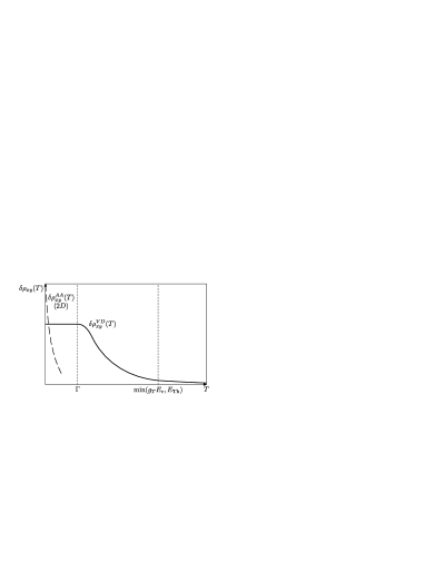
Figure 2: Temperature dependence of the Coulomb interaction corrections $\delta\rho_{xy}^{VD}(T)$ [Eq. (18)] and $\delta\rho_{xy}^{AA}(T)$ [Eq. (19)] to the Hall resistivity [second and third terms in Eq. (22), respectively]. The most significant contribution in a wide range of temperatures [$T\lesssim\min(g_{T}E_{c},E_{\text{Th}})$] both for two- and three-dimensional samples comes from the correction $\delta\rho_{xy}^{VD}(T)$ (thick solid line), which is due to the process of “virtual diffusion” of electrons through a single grain. The contribution $\delta\rho_{xy}^{VD}(T)$ is of local origin and absent in homogeneously disordered metals. It depends logarithmically on temperature $T$ in the range $\Gamma\lesssim T\lesssim\min(g_{T}E_{c},E_{\text{Th}})$, saturating at $T\sim\Gamma$ and remaining constant for $T\lesssim\Gamma$. The correction $\delta\rho_{xy}^{AA}(T)$ is analogous to the “Altshuler-Aronov” correction in ordinary disordered metals, it can be significant [Eq. (15)] for sufficiently thin granular films and low enough temperatures [$T\ll\Gamma(a/d_{z})^{2}$] only, the latter 2D case shown in figure (dashed line).

Summarizing our findings for the classical result (7), Coulomb interaction [Eqs. (9)-(11) (16)-(20)] and weak localization (21) corrections, we predict the following behavior of the Hall resistivity of a granular metal:

$$\rho_{xy}(T)=\rho_{xy}^{(0)}+\delta\rho_{xy}^{TA}+\delta\rho_{xy}^{VD}+\delta\rho_{xy}^{AA}+\delta\rho_{xy}^{WL}=$$

$$=\frac{H}{n^{*}ec}\left(1+\frac{c_{d}}{4\pi g_{T}}\ln\left[\frac{\min(g_{T}E_{c},E_{\text{Th}})}{\max(T,\Gamma)}\right]-2\frac{\delta\sigma_{xx}^{AA}(T)}{\sigma_{xx}^{(0)}}\right).$$ (22)

(i) At high enough temperatures $T\gtrsim\min(g_{T}E_{c},E_{\text{Th}})$ the Hall resistivity $\rho_{xy}(T)=\rho_{xy}^{(0)}$ is given by the Drude-like expression (7) [first term in Eq. (22)] and is independent of both the intragrain and tunnel contact disorder. Measuring $\rho_{xy}$ at such $T$ and using Eq. (7) one can extract an important characteristic of the granular system: its effective carrier density $n^{*}=An$, which is related to the actual carrier density $n$ of the grain material through a geometry-dependent factor $A\leq 1$.

(ii) In a wide temperature range $\Gamma\lesssim T\lesssim\min(g_{T}E_{c},E_{\text{Th}})$ both for 2D and 3D samples, local effects of Coulomb interaction lead to the logarithmic in $T$ correction to the Hall resistivity [$\delta\rho_{xy}^{VD}(T)$, second term in Eq. (22), see Eqs. (10),(18)]. This $\ln T$-dependence saturates at $T\sim\Gamma$ and $\delta\rho_{xy}^{VD}(T)$ remains constant for $T\lesssim\Gamma$. We emphasize that this correction is absent in homogeneously disordered metals, but it appears to be the major quantum correction to the Hall resistivity of a granular metal that governs the $T$-dependence of $\rho_{xy}(T)$ in a wide temperature range both for 2D and 3D samples.

(iii) An additional $T$-dependence of $\rho_{xy}(T)$ may arise due to the “Altshuler-Aronov” correction $\delta\sigma_{xx}^{AA}(T)$ to the longitudinal conductivity [$\delta\rho_{xy}^{AA}(T)$, third term in Eq. (22), see Eqs.  (11),(15),(19)] at much lower temperatures $T\ll\Gamma$, the most significant logarithmic contribution expected for sufficiently thin granular films [one or a few grain monolayers, Eq. (15)].

The temperature behavior of the contributions $\delta\rho_{xy}^{VD}(T)$ and $\delta\rho_{xy}^{AA}(T)$ is shown in Fig. 2.

We expect our result Eq. (22) to hold for realistic arrays with moderate structural disorder and, most importantly, with randomly distributed tunneling conductances, which is inevitable in real systems: (i) $n^{*}$ simply does not depend on the distribution of $G_{T}$; (ii) the logarithmic form of the major quantum correction [$\delta\rho_{xy}^{VD}(T)$, second term in Eq. (22)] persists in this case, although the structure factor $c_{d}\sim 1$ does depend on the distribution of conductances and $g_{T}$ should be substituted by some averaged quantity.

Comparison of our findings with experimental data may serve as a good check of the theory developed here. The experimental situation related to our theory is mentioned in the Conclusion.

III Model and Hamiltonian

We consider a quadratic ($d=2$, 2D) or cubic ($d=3$, 3D) lattice of metallic grains coupled to each other by tunnel contacts (Fig. 1).

Aiming to concentrate on the Hall effect, we assume the simplest case of translationally invariant lattice, i.e., equal tunneling conductances $G_{T}$ of all contacts, translationally invariant capacitance matrix, and identical properties of all grains (the same form and size, mean free path, electron density, density of states, etc.). After the main properties of the Hall effect in such system have been established, we argue that they also hold for realistic arrays. In real systems in the metallic regime, the major type of irregularities that (could) affect electron transport even for structurally quite regular arrays seems to be the randomness of tunneling conductances $G_{T}$, while other assumptions can be well met or are inessential.

To provide more explicit analysis we further simplify the calculations assuming the intragrain electron dynamics diffusive, i.e., that the bulk mean free path $l$ in the grain is much smaller than the size $a$ of the grain, $l\ll a$. In this case details of electron scattering off the grain boundary are irrelevant. However, our approach is also entirely applicable to the case of ballistic ($l\gtrsim a$) intragrain disorder, when surface scattering becomes important. The main results, listed in Sec. II, are valid for both diffusive and ballistic grains.

In the metallic regime ($g_{T}\gg 1$) quantum effects of Coulomb interaction can be considered perturbatively with an expansion parameter $1/g_{T}$ as long as the relative corrections remain small.

We write the Hamiltonian describing the system as

$$\hat{H}=\hat{H}_{0}+\hat{H}_{t}+\hat{H}_{c}.$$ (23)

In Eq. (23) the first term

$$\hat{H}_{0}=\sum_{\bf i}\int d{\bf r}_{\bf i}\psi^{\dagger}({\bf r}_{\bf i})\left[\xi\left({\bf p}_{\bf i}-\frac{e}{c}{\bf A}({\bf r}_{\bf i})\right)+U({\bf r}_{\bf i})\right]\psi({\bf r}_{\bf i})$$ (24)

is the Hamiltonian of isolated grains, $\xi({\bf p})={\bf p}^{2}/(2m)-\epsilon_{F}$, ${\bf A}({\bf r}_{\bf i})$ is the vector potential describing the uniform magnetic field ${\bf H}=H{\bf e}_{z}$ directed along the $z$ axis, $U({\bf r}_{\bf i})$ is the random disorder potential of the grains, ${\bf i}=(i_{1},\ldots,i_{d})~{}\in~{}\mathbb{Z}^{d}$ is an integer vector numerating the grains. The integration with respect to ${\bf r}_{\bf i}$ is done over the volume of the grain ${\bf i}$. Since we do not deal with spin-related phenomena in this paper, we omit the spin indices of the operators $\psi({\bf r}_{\bf i})$. Accounting for spin degeneracy in the course of calculations is simple: each electron loop comes with the factor 2. We consider white-noise disorder and perform averaging using the Gaussian distribution with the variance

$$\langle U({\bf r}_{\bf i})U({\bf r}^{\prime}_{\bf i})\rangle_{U}=\frac{1}{2\pi\nu\tau_{0}}\delta({\bf r}_{\bf i}-{\bf r}^{\prime}_{\bf i}),$$ (25)

where $\nu$ is the density of states in the grain at the Fermi level per one spin projection and $\tau_{0}$ is the scattering time.

The tunneling Hamiltonian $\hat{H}_{t}$ in Eq. (23) is given by

$$\hat{H}_{t}=\sum_{\langle{\bf i},{\bf j}\rangle}(X_{{\bf i},{\bf j}}+X_{{\bf j},{\bf i}}),$$ (26)

where the operator $X_{{\bf i},{\bf j}}$ describes tunneling from the grain ${\bf j}$ to the grain ${\bf i}$, the summation is taken over the neighboring grains connected by a tunnel contact, such that each contact is counted only once. For studying Hall effect the geometry of the grains and contacts is essential, therefore we write the tunneling operators $X_{{\bf i},{\bf j}}$ in the coordinate representation:

$$X_{{\bf i},{\bf j}}=\int d{\bf s}_{\bf i}d{\bf s}_{\bf j}\,t({\bf s}_{\bf i},{\bf s}_{\bf j})\psi^{\dagger}({\bf s}_{\bf i})\psi({\bf s}_{\bf j}),$$ (27)

where the integration is carried out over two surfaces of the contact: one of them (${\bf s}_{\bf i}$) belonging to the ${\bf i}$-th grain, whereas the other (${\bf s}_{\bf j}$) to the ${\bf j}$-th grain. Such form implies that tunneling occurs from a close vicinity of the contact of atomic size, but not from the bulk of the grain. This is a natural assumption, since we consider a good metallic limit for the grains, i.e., the size $a$ of the grains is much greater than the Fermi length, $p_{F}a\gg 1$ ($p_{F}$ is the Fermi momentum). Fast oscillations of the wave functions in the grains result in a fast decay of the overlap of the wave functions in different grains. Since $\hat{H}_{t}^{\dagger}=\hat{H}_{t}$, we have $X_{{\bf i},{\bf j}}^{\dagger}=X_{{\bf j},{\bf i}}$ and $t^{*}({\bf s}_{\bf i},{\bf s}_{\bf j})=t({\bf s}_{\bf j},{\bf s}_{\bf i})$.

Without further assumptions about the tunneling amplitudes $t({\bf s}_{\bf i},{\bf s}_{\bf j})$ in Eq. (27), electrons can tunnel from a given point ${\bf s}_{\bf j}$ to an arbitrary point ${\bf s}_{\bf i}$ on the other side of the contact. However, it is physically clear that (i) electrons effectively tunnel from the point ${\bf s}_{\bf j}$ to the points ${\bf s}_{\bf i}$ in the vicinity of ${\bf s}_{\bf j}$ of atomic size only, therefore $t({\bf s}_{\bf i},{\bf s}_{\bf j})$ should decay rapidly on atomic scale as a function of ${\bf s}_{\bf i}-{\bf s}_{\bf j}$; (ii) the amplitude $t({\bf s}_{\bf i},{\bf s}_{\bf j})$ can also fluctuate as a function of ${\bf s}_{\bf i}$ for fixed ${\bf s}_{\bf i}-{\bf s}_{\bf j}$ due to irregularities of the contact on atomic scale.

To effectively model this behavior of the tunneling amplitudes we consider $t({\bf s}_{\bf i},{\bf s}_{\bf j})$ as Gaussian random variables and average over them with the variance

$$\langle t({\bf s}_{\bf i},{\bf s}_{\bf j})t({\bf s}_{\bf j},{\bf s}_{\bf i})\rangle_{t}=t_{0}^{2}\delta({\bf s}_{\bf i}-{\bf s}_{\bf j}),$$ (28)

where $\delta({\bf s}_{\bf i}-{\bf s}_{\bf j})$ is an atomic scale $\delta$-function on the contact surface and $t_{0}^{2}$ has a meaning of tunneling probability per unit area of the contact. As we will see, the assumption $p_{F}a\gg 1$ will enable us to neglect the contributions containing the regular parts $\langle t({\bf s}_{\bf i},{\bf s}_{\bf j})\rangle_{t}$ of the tunneling amplitudes.

The third term in Eq. (23) stands for the Coulomb interaction between the electrons. In principle, one has to start with its the bare form

$$\hat{H}_{c}=\frac{1}{2}\sum_{{\bf i},{\bf j}}\int d{\bf r}_{\bf i}d{\bf r}_{\bf j}\,\psi^{\dagger}({\bf r}_{\bf i})\psi^{\dagger}({\bf r}_{\bf j})\frac{e^{2}}{|{\bf r}_{\bf i}-{\bf r}_{\bf j}|}\psi({\bf r}_{\bf j})\psi({\bf r}_{\bf i}).$$ (29)

Proceeding with the calculations we will have to take the screening of Coulomb potential by electron motion into account. One should distinguish between the intragrain and intergrain electron motion. In the static limit (classical electrostatics) for the intragrain motion the Coulomb interaction is reduced to the effective charging energy $E_{{\bf i}{\bf j}}$ interaction between the total excess charges of the grains. Accounting for tunneling yields the screened form of the charging energy interactionBEAH , which is sufficient for studying the intergrain transport. We will see, however, that coordinate-dependent interaction modes inside each grain arising from the intragrain motion will be necessary to get a correct frequency dependence of the classical Hall resistance $R_{H}$ of a single grain.

III.1 Kubo formula

The conductivity in a homogeneous external electric field is calculated using the Kubo formulaET in Matsubara techniqueAGD :

$$\sigma_{{\bf a}{\bf b}}(\omega)=2e^{2}a^{2-d}\frac{1}{|\omega|}\left[\Pi_{{\bf a}{\bf b}}(\omega)-\Pi_{{\bf a}{\bf b}}(0)\right]$$ (30)

$$\Pi_{{\bf a}{\bf b}}(\omega)=\sum_{\bf j}\Pi_{{\bf a}{\bf b}}(\omega,{\bf i}-{\bf j}),$$ (31)

where

$$\Pi_{{\bf a}{\bf b}}(\omega,{\bf i}-{\bf j})=\int_{0}^{1/T}d\tau\,e^{i\omega\tau}\langle T_{\tau}I_{{\bf i},{\bf a}}(\tau)I_{{\bf j},{\bf b}}(0)\rangle$$ (32)

is the current-current correlation function,

$$I_{{\bf i},{\bf a}}(\tau)=X_{{\bf i}+{\bf a},{\bf i}}(\tau)-X_{{\bf i},{\bf i}+{\bf a}}(\tau).$$ (33)

Here $\omega\in 2\pi T\mathbb{Z}$ is an external bosonic Matsubara frequency ($\mathbb{Z}$ is the set of integers), ${\bf a}$ and ${\bf b}$ are the lattice unit vectors. The factor $2$ in Eq. (30) stands for the spin degeneracy coming from one electron loop. The vector ${\bf a}$ denotes the direction of the current component and ${\bf b}$ points along the external electric field that causes the current. For example, if ${\bf b}={\bf e}_{y}$, then ${\bf a}={\bf e}_{x}$ for Hall conductivity $\sigma_{xy}=\sigma_{{\bf e}_{x}{\bf e}_{y}}$ and ${\bf a}={\bf e}_{y}$ for longitudinal conductivity $\sigma_{yy}=\sigma_{{\bf e}_{y}{\bf e}_{y}}$. Further, $A(\tau)=e^{\hat{H}\tau}Ae^{-\hat{H}\tau}$ is the Heisenberg operator in Matsubara technique. The operator of the tunneling current through the contact connecting the grains ${\bf i}$ and ${\bf i}+{\bf a}$ actually equals $-ieI_{{\bf i},{\bf a}}(\tau)$, we extracted $(-ie)^{2}$ from $\Pi_{{\bf a}{\bf b}}(\omega,{\bf i}-{\bf j})$ for further convenience. The average $\langle\ldots\rangle$ in Eq. (32) implies both the quantum mechanical thermodynamic averaging with respect to $\hat{H}$ and averaging over the intragrain and contact disorder according to Eqs. (25) and (28). The contact between the neighboring grains ${\bf i}+{\bf a}$ and ${\bf i}$ will be further identified by the pair $({\bf i}+{\bf a},{\bf i})$.

The correlation function $\Pi_{{\bf a}{\bf b}}(\omega,{\bf i}-{\bf j})$ represents the current running through the contact $({\bf i}+{\bf a},{\bf i})$ in response to the voltage applied to the contact $({\bf j}+{\bf b},{\bf j})$ only. The sum over ${\bf j}$ in Eq. (31) means that the contributions from all contacts have to be considered.

IV Technique

The current-current correlation function $\Pi_{{\bf a}{\bf b}}(\omega,{\bf i}-{\bf j})$ is calculated using diagrammatic technique. Let us first discuss its details neglecting the Coulomb interaction $\hat{H}_{c}$ [Eq. (29)] in $\hat{H}$ [Eq. (23)] completely. Technically, for a given pair $({\bf i}+{\bf a},{\bf i})$ and $({\bf j}+{\bf b},{\bf j})$ of contacts one expands Eq. (32) both in the disorder potential $U({\bf r}_{\bf i})$ [Eq. (24)] and tunnelling Hamiltonian $\hat{H}_{t}$ [Eqs. (26) and (27)]. Each diagrammatic contribution to $\Pi_{{\bf a}{\bf b}}(\omega,{\bf i}-{\bf j})$ is a loop of two Green functions connecting the contacts $({\bf i}+{\bf a},{\bf i})$ and $({\bf j}+{\bf b},{\bf j})$. Then one averages this loop over the intragrain and contact disorder according to Eqs. (25) and (28).

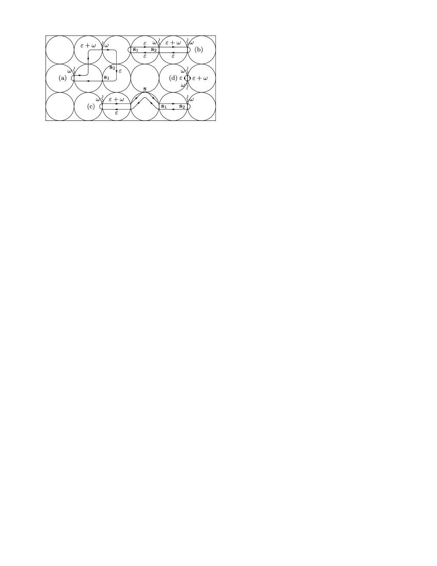
Figure 3: Different types of diagrams for the current-current correlation function $\Pi_{{\bf a}{\bf b}}(\omega,{\bf i}-{\bf j})$ [Eq. (32)] neglecting Coulomb interaction [Eq. (29)]. Diagrams of types (a) and (b) that contain oscillating at Fermi wavelength $\lambda_{F}=p_{F}^{-1}$ functions in coordinate representation vanish after the integration of the contacts surfaces give 0. In diagram (a) two different contacts are connected by a single Green function $\mathcal{G}(\varepsilon,{\bf s}_{1},{\bf s}_{2})$; in diagram (b) two different contacts are connected by two Green functions $\mathcal{G}(\varepsilon,{\bf s}_{1},{\bf s}_{2})$ and $\mathcal{G}(\varepsilon,{\bf s}_{2},{\bf s}_{1})$ having the same (sign of) energies. (c) The only type of “allowed” diagrams that do not contain oscillating functions and give nonvanishing contributions: the two contacts $({\bf i}+{\bf a},{\bf i})$ and $({\bf j}+{\bf b},{\bf j})$ with external tunneling vertices (wavy lines) are “capped” by the Green functions $G(\varepsilon,{\bf s},{\bf s})$ from one of their sides and connected by two Green functions $\mathcal{G}(\varepsilon+\omega,{\bf s}_{{\bf i}+{\bf a}},{\bf s}_{\bf j})$ and $\mathcal{G}(\varepsilon,{\bf s}_{\bf j},{\bf s}_{{\bf i}+{\bf a}})$, the “paths” of which through other contacts coincide. For energies, such that $(\varepsilon+\omega)\varepsilon<0$, the diffuson $D$ [Eq. (34)] in each grain along this path arises. (d) Diagram for the longitudinal conductivity $\sigma_{xx}^{(0)}=a^{2-d}G_{T}$ [Eq. (4)] in the leading order in $g_{T}/g_{0}\ll 1$.

Of course, many different possibilities of drawing such loop can be considered (see Fig. 3). However due to the general properties of the Green functions in the coordinate representation and the assumption employed in Eq. (27) that tunneling occurs from the vicinity of the contacts, but not from the bulk of the grain, a lot of them can be ruled out even before averaging over $U({\bf r})$.

Consider a Matsubara Green function $\mathcal{G}(\varepsilon,{\bf r},{\bf r}^{\prime})$ of an arbitrary grain for a given realization of the disorder potential $U({\bf r})$. The Green function $\mathcal{G}(\varepsilon,{\bf r},{\bf r}^{\prime})\propto e^{ip_{F}|{\bf r}-{\bf r}^{\prime}|\text{sgn}\,\varepsilon}$ oscillates at the Fermi wavelength $\lambda_{F}=p_{F}^{-1}$ as a function of the difference ${\bf r}-{\bf r}^{\prime}$. Since we assume the grain size $a$ and the size of the area of the contact much greater than $\lambda_{F}$, this fact excludes the following possibilities.

(i) If two different contacts ${\bf s}_{1}$ and ${\bf s}_{2}$ are connected by a single Green function $\mathcal{G}(\varepsilon,{\bf s}_{1},{\bf s}_{2})$ in a given grain (Fig. 3a), then integration over the contacts surfaces $\int d{\bf s}_{1}d{\bf s}_{2}\mathcal{G}(\varepsilon,{\bf s}_{1},{\bf s}_{2})$ gives zero due to the rapid oscillations of the integrand.

(ii) If two different contacts ${\bf s}_{1}$ and ${\bf s}_{2}$ are connected by two Green functions $\mathcal{G}(\varepsilon,{\bf s}_{1},{\bf s}_{2})$ and $\mathcal{G}(\varepsilon^{\prime},{\bf s}_{2},{\bf s}_{1})$ (or $\mathcal{G}(\varepsilon^{\prime},{\bf s}_{1},{\bf s}_{2})$) in a given grain having the same signs of energies, $\varepsilon\varepsilon^{\prime}>0$, (Fig. 3b) then, again, their product is an oscillating function and $\int d{\bf s}_{1}d{\bf s}_{2}\mathcal{G}(\varepsilon,{\bf s}_{1},{\bf s}_{2})\mathcal{G}(\varepsilon^{\prime},{\bf s}_{2},{\bf s}_{1})$ also gives zero.

So, the only objects of the diagrammatic technique that “survive” inside the grains are those that do not contain oscillations at the Fermi wavelength $\lambda_{F}$ in their coordinate dependence (Fig.3c). These are: (1) the single Green function $\mathcal{G}(\varepsilon,{\bf s},{\bf s})$ with coinciding coordinates ${\bf s}$ on the contact surface; (2) the product of two Green functions with pairwise coinciding coordinates and opposite signs of energies: $\mathcal{G}(\varepsilon,{\bf s}_{1},{\bf s}_{2})\mathcal{G}(\varepsilon^{\prime},{\bf s}_{2},{\bf s}_{1})$ or $\mathcal{G}(\varepsilon,{\bf s}_{1},{\bf s}_{2})\mathcal{G}(\varepsilon^{\prime},{\bf s}_{1},{\bf s}_{2})$ with $\varepsilon\varepsilon^{\prime}<0$. After disorder averaging such products of two Green function give well-known electron propagators for a single isolated grain: the “diffuson”

$$D(\omega,{\bf r},{\bf r}^{\prime})\equiv\frac{1}{2\pi\nu}\langle\mathcal{G}(\varepsilon+\omega,{\bf r},{\bf r}^{\prime})\mathcal{G}(\varepsilon,{\bf r}^{\prime},{\bf r})\rangle_{U},\mbox{ }(\varepsilon+\omega)\varepsilon<0.$$ (34)

and the “Cooperon”

$$C(\omega,{\bf r},{\bf r}^{\prime})\equiv\frac{1}{2\pi\nu}\langle\mathcal{G}(\varepsilon+\omega,{\bf r},{\bf r}^{\prime})\mathcal{G}(\varepsilon,{\bf r},{\bf r}^{\prime})\rangle_{U},\mbox{ }(\varepsilon+\omega)\varepsilon<0.$$

Cooperons will be important for weak localization effects KEprepWL , while in this paper we only consider the diffuson (34) in detail.

We are left with the following general type of diagram (in the absence of Coulomb interaction and weak localization effects) for $\Pi_{{\bf a}{\bf b}}(\omega,{\bf i}-{\bf j})$ shown in Fig.3c: (1) each contact $({\bf i}+{\bf a},{\bf i})$ and $({\bf j}+{\bf b},{\bf j})$ with external tunneling vertices must be “capped” by the Green function $G(\varepsilon,{\bf s},{\bf s})$ from one of its sides (one cannot “construct” a diffuson from $G(\varepsilon,{\bf s},{\bf s})$, since only one energy $\varepsilon$ is available, see Fig. 3b); (2) two Green functions $\mathcal{G}(\varepsilon+\omega,{\bf s}_{{\bf i}+{\bf a}},{\bf s}_{\bf j})$ and $\mathcal{G}(\varepsilon,{\bf s}_{\bf j},{\bf s}_{{\bf i}+{\bf a}})$ connect the contacts $({\bf i}+{\bf a},{\bf i})$ and $({\bf j}+{\bf b},{\bf j})$ from the opposite sides and their “paths” through different contacts must coincide. Therefore, in each grain along this path the diffuson $D$ [Eq. (34)] of this particular grain arises. The arising product of two Green functions with pairwise coinciding coordinates defines the diffuson of the whole granular system

$$\mathcal{D}(\omega,{\bf r}_{\bf i},{\bf r}^{\prime}_{\bf j})\equiv\frac{1}{2\pi\nu}\langle\mathcal{G}(\varepsilon+\omega,{\bf r}_{\bf i},{\bf r}^{\prime}_{\bf j})\mathcal{G}(\varepsilon,{\bf r}^{\prime}_{\bf j},{\bf r}_{\bf i})\rangle_{U,t},\mbox{ }(\varepsilon+\omega)\varepsilon<0.$$ (35)

Contrary to Eq. (34), the points ${\bf r}_{\bf i}$ ${\bf r}^{\prime}_{\bf j}$ may belong to different distant grains ${\bf i}$ and ${\bf j}$ now. Each diagrammatic contribution to $\mathcal{D}$ [Eq. (35)] is factorized into the product of intragrain diffusons $D$ [Eq. (34)] connecting different contacts inside the grain and tunneling probabilities expressed via the tunneling escape rate $\Gamma$.

To get the conductivity $\sigma_{{\bf a}{\bf b}}(\omega)$ one should sum $\Pi_{{\bf a}{\bf b}}(\omega,{\bf i}-{\bf j})$ over all ${\bf j}$ according to Eq. (31). An important observation is that due to this summation the intragrain diffusons always enter the expression for $\sigma_{{\bf a}{\bf b}}(\omega)$ as a difference $D(\omega,{\bf s}_{1},{\bf s}_{2})-D(\omega,{\bf s}_{3},{\bf s}_{4})$ of the diffusons connecting different contacts Therefore the zero mode $1/(|\omega|\mathcal{V})$ (see Sec. IV.1 below) drops out and the contribution to $\sigma_{{\bf a}{\bf b}}(\omega)$ comes from nonzero modes with “excitation energies” of the order of the Thouless energy $E_{\text{Th}}$. Each pair “grain + contact” brings a factor $\Gamma/E_{\text{Th}}\propto g_{T}/g_{0}$, given by the ratio of the tunneling conductance $g_{T}$ to the conductance of the grain $g_{0}$.

What does the above procedure amount to? It appears, that this procedure reproduces exactly the solution of the classical electrodynamics problem for the conductivity of a granular medium, provided each tunnel contact is viewed as a surface resistor with conductance $G_{T}$ . In principle, this approach allows one to study both LC and HC of the granular system for arbitrary ratio $g_{T}/g_{0}$. For example, the classical formula

$$\sigma^{(0)}_{xx}=a^{2-d}\frac{G_{T}G_{0}}{G_{T}+G_{0}}$$

for LC can be obtained (the contact $G_{T}^{-1}$ and grain $G_{0}^{-1}$ resistances connected in series). Its expansion

$$\sigma^{(0)}_{xx}=a^{2-d}(G_{T}-G_{T}^{2}/G_{0}+G_{T}^{3}/G_{0}^{2}-\ldots)$$ (36)

in $g_{T}/g_{0}$ corresponds to the expansion of the diffuson $\mathcal{D}$ in the intragrain diffusons $D$. Each subsequent term in Eq. (36) corresponds to including contacts $({\bf j}+{\bf e}_{x},{\bf j})$ more and more remote from $({\bf i}+{\bf e}_{x},{\bf i})$ in Eq. (31).

However, for the system with well-pronounced granularity [$g_{T}\ll g_{0}$, Eqs. (2) and (3)] one does not need to sum the contributions from all distant contacts $({\bf j}+{\bf b},{\bf j})$ in Eq. (31).

It is sufficient to consider the lowest nonvanishing order in $g_{T}/g_{0}\ll 1$, given by the closest contacts. In fact, for LC $\sigma_{xx}^{(0)}$ (${\bf a}={\bf b}={\bf e}_{x}$) considering non-zero-mode intragrain diffusons is not necessary at all, since the first term $G_{T}$ [Eq. (4)] of the expansion (36) is obtained from a single contact (${\bf j}={\bf i}$) without expanding Eq. (32) in $\hat{H}_{t}$ (see Fig. 3d). Including the closest contacts (${\bf j}={\bf i},{\bf i}\pm{\bf e}_{x}$ in Eq. (31)) via the intragrain diffusons $D$ will give the next term $-G_{T}^{2}/G_{0}$ in Eq. (36), which is a small correction to $G_{T}$.

On the contrary, for the Hall conductivity $\sigma_{xy}$ (${\bf a}={\bf e}_{x},{\bf b}={\bf e}_{y}$) the expansion in $g_{T}/g_{0}$ starts from the term $G_{T}^{2}R_{H}$ [Eq. (5)] analogous to $-G_{T}^{2}/G_{0}$ in Eq. (36). To get this term one must connect the contacts $({\bf j}+{\bf e}_{y},{\bf j})$ in the $y$ direction closest to the contact $({\bf i}+{\bf e}_{x},{\bf i})$ in the $x$ direction via the intagrain diffusons $D$ [i.e., take into account the terms with ${\bf j}={\bf i}-{\bf e}_{y},{\bf i},{\bf i}+{\bf e}_{x},{\bf i}+{\bf e}_{x}-{\bf e}_{y}$ in Eq. (31)]. Thus, considering nonzero diffusion modes for Hall transport is inevitable.

The above considerations also explain why expanding in the tunneling Hamitonian $\hat{H}_{t}$ is a “legal” procedure in the metallic regime, even though the dimensionless tunneling coupling constant $g_{T}\gg 1$ is large. The answer is that the actual expansion parameter is the ratio $g_{T}/g_{0}$.

Before we proceed with the Hall conductivity, we consider important building blocks of our diagrammatic technique: the intragrain diffuson in the presence of magnetic field and the screened Coulomb interaction.

IV.1 Intragrain diffuson

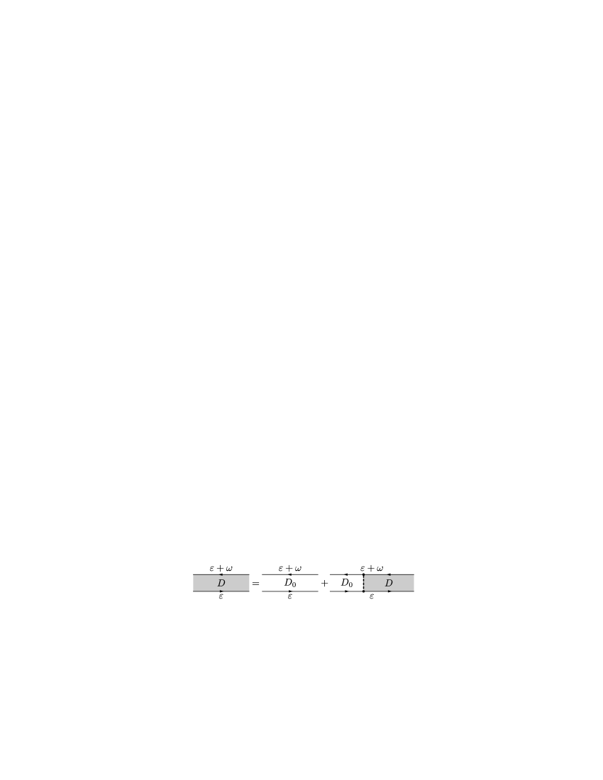
Figure 4: Diagrammatic representation of the integral equation (37) for the diffuson $D(\omega,{\bf r},{\bf r}^{\prime})$ (gray block), defined by Eq. (34). Fermionic lines stand for the disorder-averaged Green function $G(\varepsilon,{\bf r},{\bf r}^{\prime})$, dashed line denotes the correlation function (25) of the random potential.

The diffuson $D(\omega,{\bf r},{\bf r}^{\prime})$ of a single isolated grain is defined by Eq. (34). The averaging over the disorder potential $U({\bf r})$ in Eq. (34) is done using the conventional diagrammatic technique AGD . In the “noncrossing” approximation valid for weak disorder ($p_{F}l\gg 1$, where $l=v_{F}\tau_{0}$ is the electron mean free path and $v_{F}$ is the Fermi velocity) the diffuson is given by the sum of ladder-type diagrams. This standard series can be expressed in terms of the solution of the integral equation (Fig. 4)

$$D(\omega,{\bf r},{\bf r}^{\prime})=D_{0}(\omega,{\bf r},{\bf r}^{\prime})+\frac{1}{\tau_{0}}\int d{\bf x}D_{0}(\omega,{\bf r},{\bf x})D(\omega,{\bf x},{\bf r}^{\prime}),$$ (37)

where

$$D_{0}(\omega,{\bf r},{\bf r}^{\prime})=\frac{1}{2\pi\nu}G(\varepsilon+\omega,{\bf r},{\bf r}^{\prime})G(\varepsilon,{\bf r}^{\prime},{\bf r})$$

is the “ladder step” and $G(\varepsilon+\omega,{\bf r},{\bf r}^{\prime})=\langle\mathcal{G}(\varepsilon+\omega,{\bf r},{\bf r}^{\prime})\rangle_{U}$ is the disorder-averaged Green function of the grain.

In the diffusive limit ($l\ll a$, $\omega\tau_{0}\ll 1$) the integral equation (37) can be reduced to the differential diffusion equation (we assume $\omega\geq 0$ from now on)

$$(\omega-D_{0}\nabla_{\bf r}^{2})D(\omega,{\bf r},{\bf r}^{\prime})=\delta({\bf r}-{\bf r}^{\prime})$$ (38)

where $D_{0}=v_{F}l/3$ is the classical diffusion coefficient in the grain ($D_{0}$ is not affected by magnetic field, such that $\omega_{H}\tau_{0}\ll 1$). Equation (38) must be supplied by a proper boundary condition at the grain surface, which we derive in Appendix A in the presence of magnetic field:

$$({\bf n},\nabla_{\bf r}D)|_{{\bf r}\in S}=\omega_{H}\tau_{0}({\bf t},\nabla_{\bf r}D)|_{{\bf r}\in S}.$$ (39)

Here ${\bf n}$ is the normal unit vector pointing outside the grain, ${\bf t}=[{\bf n},{\bf H}]/H$ is the tangent vector pointing in the direction opposite to the edge drift. Equation (39) is due to the fact that the current component normal to the grain surface vanishes, its RHS describes the edge drift caused by the magnetic part of the Lorentz force. Note that only due to the boundary condition (39) the diffuson $D$ “knows” about the magnetic field. All information about the magnetic field in the system is now contained in this boundary condition and the nonzero HC we will obtain is due to the nonzero RHS of Eq. (39) only. The main consequence of Eq. (39), crucial for the Hall effect, is the directional asymmetry

$$D(\omega,{\bf r},{\bf r}^{\prime})\neq D(\omega,{\bf r}^{\prime},{\bf r})$$

of the diffuson for $H\neq 0$. For $H=0$, Eq. (39) reduces to the well-known Neumann boundary condition.

The solution to Eqs. (38) and (39) can be presented in the form

$$D(\omega,{\bf r},{\bf r}^{\prime})=\frac{1}{\omega\mathcal{V}}+\sum_{n>0}\frac{\phi_{n}({\bf r})\phi^{*}_{n}({\bf r}^{\prime})}{\omega+\gamma_{n}},$$ (40)

where $\phi_{n}$ are the eigenfunctions of the problem

$$-\nabla_{\bf r}^{2}\phi_{n}=q^{2}_{n}\phi_{n},\mbox{ }({\bf n},\nabla_{\bf r}\phi_{n})|_{S}=\omega_{H}\tau_{0}({\bf t},\nabla_{\bf r}\phi_{n})|_{S},$$

$\gamma_{n}=D_{0}q_{n}^{2}$ is the “diffusion spectrum”, and $\mathcal{V}$ is the grain volume. The functions $\phi_{n}$ satisfy the orthonormality condition

$$\int d{\bf r}\phi_{n}^{*}({\bf r})\phi_{n^{\prime}}({\bf r})=\delta_{nn^{\prime}}.$$ (41)

There always exists a uniform solution $\phi_{0}({\bf r})=1/\sqrt{\mathcal{V}}$ with the zero eigenvalue $\gamma_{0}=0$ giving the zero mode $1/(\omega\mathcal{V})$ in Eq. (40). The lowest excited mode $\gamma_{1}\sim E_{\text{Th}}\equiv D_{0}/a^{2}$ defines the Thouless energy scale $E_{\text{Th}}$. The zero mode $1/(\omega\mathcal{V})$ describes the fact that at time scales much greater than the traversal time $1/E_{\text{Th}}$ the probability density to find an electron is distributed uniformly over the grain volume. Information about nontrivial intragrain dynamics is contained in nonzero modes:

$$\bar{D}(\omega,{\bf r},{\bf r}^{\prime})=\sum_{n>0}\frac{\phi_{n}({\bf r})\phi^{*}_{n}({\bf r}^{\prime})}{\omega+\gamma_{n}}.$$ (42)

We will see that for Hall effect, for which the intragrain dynamics is essential, only the non-zero mode part $\bar{D}(\omega,{\bf r},{\bf r}^{\prime})$ of the diffuson $D(\omega,{\bf r},{\bf r}^{\prime})$ enters the expressions for HC and HR, whereas the zero mode $1/(\omega\mathcal{V})$ simply drops out.

IV.2 Screened Coulomb interaction

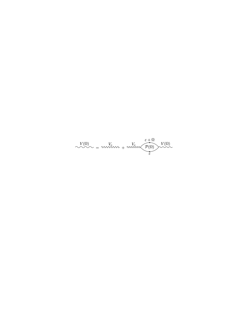
Figure 5: Diagrammatic representation of the integral equation (43) for the screened Coulomb interaction $V(\Omega,{\bf r}_{\bf i},{\bf r}^{\prime}_{\bf j})$ [wavy line, see Eqs. (52),(53),(49) below]. Zigzag line represents the bare Coulomb potential $V_{c}({\bf r}-{\bf r}^{\prime})=e^{2}/|{\bf r}-{\bf r}^{\prime}|$ and electron loop the polarization operator $\mathcal{P}(\Omega,{\bf r}_{\bf i},{\bf r}^{\prime}_{\bf j})$ [Eq. (44)].

Within the random phase approximation the screened Coulomb interaction is given by a diagrammatic series, that can be obtained as a solution of the integral equation (Fig. 5)

$$V(\Omega,{\bf r}_{\bf i},{\bf r}^{\prime}_{\bf j})=V_{c}({\bf r}_{\bf i}-{\bf r}^{\prime}_{\bf j})-\sum_{{\bf k},{\bf l}}\int d{\bf x}_{\bf k}d{\bf x}^{\prime}_{\bf l}\times$$

$$\times V_{c}({\bf r}_{\bf i}-{\bf x}_{\bf k})\,\nu\mathcal{P}(\Omega,{\bf x}_{\bf k},{\bf x}^{\prime}_{\bf l})\,V(\Omega,{\bf x}^{\prime}_{\bf l},{\bf r}^{\prime}_{\bf j}),$$ (43)

where $\Omega\in 2\pi T\mathbb{Z}$ is a bosonic Matsubara frequency and $V_{c}({\bf r}-{\bf r}^{\prime})=e^{2}/|{\bf r}-{\bf r}^{\prime}|$ is the bare Coulomb interaction Eq. (29). Just like for ordinary disordered metals the polarization operator of the granular system is defined as an electron-hole loop

$$\mathcal{P}(\Omega,{\bf r}_{\bf i},{\bf r}^{\prime}_{\bf j})=-\frac{2}{\nu}T\sum_{\varepsilon}\langle\mathcal{G}(\varepsilon+\Omega,{\bf r}_{\bf i},{\bf r}^{\prime}_{\bf j})\mathcal{G}(\varepsilon,{\bf r}^{\prime}_{\bf j},{\bf r}_{\bf i})\rangle_{U,t}$$ (44)

(2 comes from the spin degeneracy) and can be expressed in terms of the diffuson (35) of the system (we assume $\Omega\geq 0$):

$$\mathcal{P}(\Omega,{\bf r}_{\bf i},{\bf r}^{\prime}_{\bf j})=2\left[\delta_{{\bf i}{\bf j}}\delta({\bf r}_{\bf i}-{\bf r}^{\prime}_{\bf j})-\Omega\mathcal{D}(\Omega,{\bf r}_{\bf i},{\bf r}^{\prime}_{\bf j})\right]$$ (45)

Since the Coulomb potential $V_{c}({\bf r}-{\bf r}^{\prime})$ satisfies the Poisson equation

$$-\nabla_{\bf r}^{2}V_{c}({\bf r}-{\bf r}^{\prime})=4\pi e^{2}\delta({\bf r}-{\bf r}^{\prime})$$

Eq. (43) can be rewritten in a differential form

$$-r_{D}^{2}\nabla_{\bf r}^{2}V(\Omega,{\bf r}_{\bf i},{\bf r}^{\prime}_{\bf j})=\frac{1}{\nu}\delta_{{\bf i}{\bf j}}\delta({\bf r}_{\bf i}-{\bf r}^{\prime}_{\bf j})-$$

$$-\sum_{{\bf k}}\int d{\bf x}_{\bf k}\mathcal{P}(\Omega,{\bf r}_{\bf i},{\bf x}_{\bf k})V(\Omega,{\bf x}_{\bf k},{\bf r}^{\prime}_{\bf j}),$$ (46)

where $r_{D}$ is the Debye screening radius, $1/r_{D}^{2}=4\pi e^{2}\nu$.

Depending on the approximations used for $\mathcal{D}$, one obtains different forms of the screened potential $V(\Omega,{\bf r}_{\bf i},{\bf r}^{\prime}_{\bf j})$.

IV.2.1 Coulomb interaction $V(\Omega,{\bf r}_{\bf i},{\bf r}^{\prime}_{\bf j})$ for isolated grains

First we obtain the screened potential $V(\Omega,{\bf r}_{\bf i},{\bf r}^{\prime}_{\bf j})$ neglecting tunneling between the grains. In this case the polarization operator (45) takes the form

$$\mathcal{P}(\Omega,{\bf r}_{\bf i},{\bf r}^{\prime}_{\bf j})=\delta_{{\bf i}{\bf j}}P(\Omega,{\bf r}_{\bf i},{\bf r}^{\prime}_{\bf j}),$$

where

$$P(\Omega,{\bf r},{\bf r}^{\prime})=2\left[\delta({\bf r}-{\bf r}^{\prime})-\Omega D(\Omega,{\bf r},{\bf r}^{\prime})\right]$$

is the polarization operator of a single isolated grain:

$$P(\Omega,{\bf r},{\bf r}^{\prime})=\sum_{n>0}P_{n}(\Omega)\phi_{n}({\bf r})\phi^{*}_{n}({\bf r}^{\prime}),\mbox{ }P_{n}(\Omega)=2\frac{\gamma_{n}}{\Omega+\gamma_{n}},$$ (47)

[see Eq. (40)]. Considering the limit when (i) the spatial scales $q_{n}^{-1}\sim a\gg r_{D}$ are much greater than the Debye screening radius $r_{D}$, (ii) the frequencies $\Omega\ll\sigma_{xx}^{\text{gr}}$ are much smaller than the grain conductivity $\sigma_{xx}^{\text{gr}}$ ($\sigma_{xx}^{\text{gr}}\propto D_{0}/r_{D}^{2}$), we can neglect the LHS of Eq. (46) altogether. Following the lines of Ref. ABG, , we get

$$V(\Omega,{\bf r}_{\bf i},{\bf r}^{\prime}_{\bf j})=E_{{\bf i}{\bf j}}+\delta_{{\bf i}{\bf j}}\,v(\Omega,{\bf r}_{\bf i},{\bf r}^{\prime}_{\bf j}).$$ (48)

Here $E_{{\bf i}{\bf j}}=e^{2}(C^{-1})_{{\bf i}{\bf j}}$ is the charging energy matrix of the granular array ($C_{{\bf i}{\bf j}}$ is the capacitance matrix, see e.g. Ref. LLECM, ). The characteristic scale of $E_{{\bf i}{\bf j}}$ is $E_{c}=e^{2}/(\kappa a)$, where $\kappa$ is the dielectric constant of the array. The charging energy $E_{{\bf i}{\bf j}}$ appears from the zero mode $1/(\Omega\mathcal{V})$ of the diffuson $D(\Omega,{\bf r},{\bf r}^{\prime})$. On the contrary, the coordinate-dependent part of the interaction inside the grain is due to the nonzero diffusion modes of $D(\Omega,{\bf r},{\bf r}^{\prime})$ and equals

$$v(\Omega,{\bf r},{\bf r}^{\prime})=\frac{1}{\nu}\sum_{n>0}v_{n}(\Omega)\phi_{n}({\bf r})\phi^{*}_{n}({\bf r}^{\prime}),\mbox{ }v_{n}(\Omega)=\frac{1}{2}\frac{\Omega+\gamma_{n}}{\gamma_{n}}.$$ (49)

For $q_{n}r_{D}\ll 1$ and $\Omega\ll\sigma_{xx}^{\text{gr}}$ this part is completely screened and equal to the inverse intragrain polarization operator (47), $v_{n}(\Omega)=1/[P_{n}(\Omega)]$.

IV.2.2 Coulomb interaction $V(\Omega,{\bf r}_{\bf i},{\bf r}^{\prime}_{\bf j})$ taking tunneling into account

Now we take tunneling into account. This modifies the expression for the diffuson $\mathcal{D}(\Omega,{\bf r}_{\bf i},{\bf r}^{\prime}_{\bf j})$ in Eq. (44), which now becomes nondiagonal in the grain indices ${\bf i},{\bf j}$. Let us rewrite the diffuson $\mathcal{D}$ in the following form:

$$\mathcal{D}(\Omega,{\bf r}_{\bf i},{\bf r}^{\prime}_{\bf j})=\delta_{{\bf i}{\bf j}}D(\Omega,{\bf r}_{\bf i},{\bf r}^{\prime}_{\bf j})+\delta D(\Omega,{\bf r}_{\bf i},{\bf r}^{\prime}_{\bf j}).$$

The part $\delta D(\Omega,{\bf r}_{\bf i},{\bf r}^{\prime}_{\bf j})$ is responsible for tunneling and vanishes, if tunneling is absent. If we leave only the zero intragrain modes (0D limit) in $\delta D(\Omega,{\bf r}_{\bf i},{\bf r}^{\prime}_{\bf j})$, the diffuson equals

$$\mathcal{D}(\Omega,{\bf r}_{\bf i},{\bf r}^{\prime}_{\bf j})=\delta_{{\bf i}{\bf j}}\bar{D}(\Omega,{\bf r}_{\bf i},{\bf r}^{\prime}_{\bf j})+\frac{1}{\mathcal{V}}\mathcal{D}_{0}(\Omega,{\bf i},{\bf j}),$$ (50)

where $\bar{D}(\Omega,{\bf r},{\bf r}^{\prime})$ [Eq. (42)] is the non-zero-mode part of the intragrain diffuson and

$$\mathcal{D}_{0}(\Omega,{\bf i},{\bf j})=\sum_{\bf q}e^{ia{\bf q}({\bf i}-{\bf j})}\mathcal{D}_{0}(\Omega,{\bf q}),$$

$$\mathcal{D}_{0}(\Omega,{\bf q})=1/(\Omega+\Gamma_{\bf q}),$$ (51)

is the diffuson for the whole granular system with 0D limit in each grain. The “kinetic term” $\Gamma_{\bf q}$ in Eq. (51) equals

$$\Gamma_{\bf q}=2\Gamma\sum_{\beta}(1-\cos q_{\beta}a),$$

where $\Gamma=2\pi\nu t_{0}^{2}S_{0}/\mathcal{V}$ is the tunneling escape rate ($S_{0}$ is the area of the contact), $\beta=x,y$ for $d=2$ and $\beta=x,y,z$ for $d=3$, ${\bf q}\in[-\pi/a,\pi/a]^{d}$ is the quasimomentum of the granular lattice, and the sum $\sum_{\bf q}\ldots=\int\frac{a^{d}d^{d}{\bf q}}{(2\pi)^{d}}\ldots$ denotes the integration over the first Brillouin zone $[-\pi/a,\pi/a]^{d}$ .

According to Eq. (50) the polarization operator (45) takes the form

$$\mathcal{P}(\Omega,{\bf r}_{\bf i},{\bf r}^{\prime}_{\bf j})=\delta_{{\bf i}{\bf j}}P(\Omega,{\bf r}_{\bf i},{\bf r}^{\prime}_{\bf j})+\frac{1}{\mathcal{V}}\mathcal{P}_{0}(\Omega,{\bf i},{\bf j}),$$

where

$$\mathcal{P}_{0}(\Omega,{\bf i},{\bf j})=2\left[\delta_{{\bf i}{\bf j}}-\Omega\mathcal{D}_{0}(\Omega,{\bf i},{\bf j})\right],\mbox{ }\mathcal{P}_{0}(\Omega,{\bf q})=2\frac{\Gamma_{\bf q}}{\Omega+\Gamma_{\bf q}}$$

is the zero-mode polarization operator of a granular systemBEAH .

Accounting for tunneling according to Eq. (50) results in the screening of the charging energy $E_{{\bf i}{\bf j}}$ in Eq. (48) only, whereas $v(\Omega,{\bf r}_{\bf i},{\bf r}^{\prime}_{\bf j})$ remains unchanged. As a result, we get for the screened Coulomb interaction of the granular system:

$$V(\Omega,{\bf r}_{\bf i},{\bf r}^{\prime}_{\bf j})=V(\Omega,{\bf i},{\bf j})+\delta_{{\bf i}{\bf j}}\,v(\Omega,{\bf r}_{\bf i},{\bf r}^{\prime}_{\bf j}),$$ (52)

where

$$V(\Omega,{\bf i},{\bf j})=\sum_{\bf q}e^{ia{\bf q}({\bf i}-{\bf j})}V(\Omega,{\bf q})$$

is the screened form of the zero-mode interaction BEAH ,

$$V(\Omega,{\bf q})=\frac{E_{c}({\bf q})}{1+[E_{c}({\bf q})/\delta]\mathcal{P}_{0}(\Omega,{\bf q})},$$ (53)

$$E_{c}({\bf q})=\sum_{\bf i}e^{-ia{\bf q}({\bf i}-{\bf j})}E_{{\bf i}-{\bf j}},$$

and $v(\Omega,{\bf r},{\bf r}^{\prime})$ is given by Eq. (49).

The form (52) of the screened interaction will be sufficient for us. We will see that the nonzero interaction modes $v(\Omega,{\bf r},{\bf r}^{\prime})$ inside the grain will be necessary to get a correct classical expression for the Hall resistance $R_{H}$ of the grain and the screened zero-mode interaction $V(\Omega,{\bf i},{\bf j})$ will be sufficient for calculating quantum corrections to the classical result. Significant quantum corrections to HC and HR arise from the frequency range $\Omega\ll g_{T}E_{c}$ ($g_{T}E_{c}$ is the inverse $RC$-time of the pair “contact+grain”), when $V(\Omega,{\bf i},{\bf j})$ is completely screened by the intergrain motion:

$$V(\Omega,{\bf q})=\frac{\delta}{\mathcal{P}_{0}(\Omega,{\bf q})}=\frac{\delta}{2}\frac{\Omega+\Gamma_{\bf q}}{\Gamma_{\bf q}},\mbox{ }\Omega\ll g_{T}E_{c}.$$

V Hall conductivity

Having obtained important building blocks of the diagrammatic technique, the intragrain diffuson and screened Coulomb interaction, we can proceed with our main goal: calculating Hall conductivity.

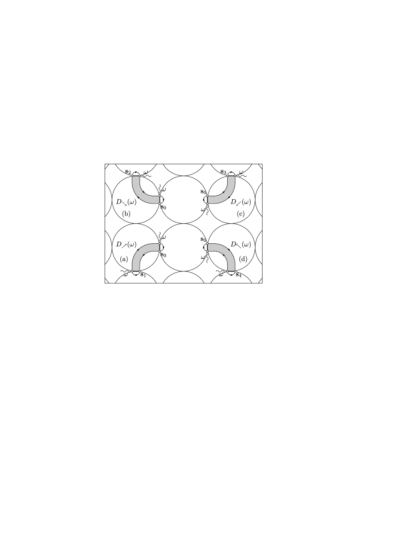
Figure 6: Diagrams giving the contribution $\sigma_{xy}^{(0,1)}(\omega)$ [Eq. (62)] to the bare (without quantum effects) Hall conductivity $\sigma_{xy}^{(0)}(\omega)$ [Eq. (68)] of the granular metal. The contacts ${\bf s}_{a}$, $a=1,2,3,4$, must be connected to the contact ${\bf s}_{0}$ by the intragrain diffusons, as shown in diagrams (a), (b), (c), and (d). The diagrams are offset for clarity, the contact ${\bf s}_{0}$ in each diagrams denotes the same contact. For each diagram four possibilities of attaching external tunneling vertices (wavy lines) must be considered, as shown in Fig. 7, only one choice is shown here.

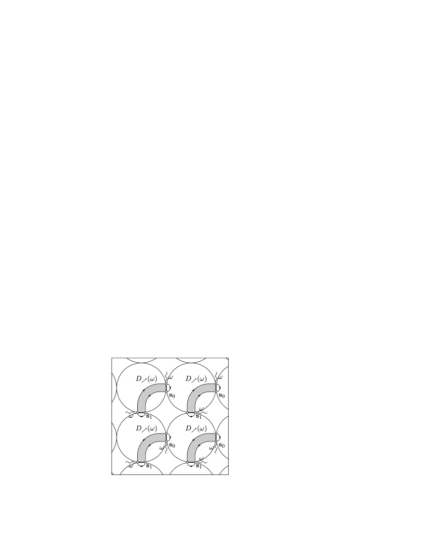
Figure 7: For each diagram in Fig. 6 four possibilities [two for each contact according to Eq. (33)] of attaching external tunneling vertices (wavy lines) must be considered.

We start by neglecting Coulomb interaction $\hat{H}_{c}$ [Eq. (29)] in $\hat{H}$ [Eq. (23)] completely. As explained in Sec. IV, in order to compute Hall conductivity $\sigma_{xy}$ (${\bf a}={\bf e}_{x},{\bf b}={\bf e}_{y}$) in the lowest nonvanishing order in $g_{T}/g_{0}\ll 1$ one has to consider the contacts $({\bf j}+{\bf e}_{y},{\bf j})$ in the $y$ direction closest to the contact $({\bf i}+{\bf e}_{x},{\bf i})$ in the $x$ direction. Calculating the current through the contact $({\bf i}+{\bf e}_{x},{\bf i})$ (denoted further ${\bf s}_{0}$) one has to connect the contacts ${\bf s}_{1},{\bf s}_{2},{\bf s}_{3},{\bf s}_{4}$ to ${\bf s}_{0}$, corresponding to ${\bf j}={\bf i}-{\bf e}_{y},{\bf i},{\bf i}+{\bf e}_{x},{\bf i}+{\bf e}_{x}-{\bf e}_{y}$ in Eqs. (31) and (32), respectively, by the diffusons $D(\omega,{\bf s}_{0},{\bf s}_{a})$, $a=1,2,3,4$, of a single grain, as shown in Fig. 6.

Let us consider the contribution $\Pi_{\nearrow}^{(0,1)}(\omega)$ to the correlation function $\Pi_{xy}[\omega,{\bf i}-({\bf i}-{\bf e}_{y})]$ [Eq. (32)] from the contact ${\bf s}_{1}$. From now on we assume $\omega\geq 0$, the arrow subscript $\nearrow$ denotes the direction of the diffuson according to Fig. 6, the superscript “0” stands for the “bare value” without quantum effects of Coulomb interaction, the superscript “1” is introduced, since there will be another contribution “2” to HC, see Sec. V.1. According to the diagram in Fig. 6, we get:

$$\Pi_{\nearrow}^{(0,1)}(\omega) = -2\pi\nu t_{0}^{4}T\sum_{-\omega<\varepsilon<0}\int d{\bf s}_{0}d{\bf s}_{1}D_{\bf i}(\omega,{\bf s}_{0},{\bf s}_{1})$$

$$\times [G_{{\bf i}+{\bf e}_{x}}(\varepsilon+\omega,{\bf s}_{0},{\bf s}_{0})-G_{{\bf i}+{\bf e}_{x}}(\varepsilon,{\bf s}_{0},{\bf s}_{0})]$$

$$\times [G_{{\bf i}-{\bf e}_{y}}(\varepsilon+\omega,{\bf s}_{1},{\bf s}_{1})-G_{{\bf i}-{\bf e}_{y}}(\varepsilon,{\bf s}_{1},{\bf s}_{1})].$$

Each end of the diffuson $D_{\bf i}$ of the grain ${\bf i}$ is “capped” by the Green functions $G_{{\bf i}+{\bf e}_{x}}$ and $G_{{\bf i}-{\bf e}_{y}}$ of the adjacent grains ${\bf i}+{\bf e}_{x}$ and ${\bf i}-{\bf e}_{y}$. We do not write the grain subscripts further. The difference $G(\varepsilon+\omega)-G(\varepsilon)$ for each contact arises due to two possibilities of choosing the external tunneling vertex in $I_{{\bf i},{\bf a}}$: $X_{{\bf i}+{\bf a},{\bf i}}$ or $-X_{{\bf i},{\bf i}+{\bf a}}$, see Eq. (33) and Fig. 7. For the Green functions at coinciding points one can use their bulk expression (with $H=0$) $G^{-1}(\varepsilon,{\bf p})=i\varepsilon-\xi({\bf p})+\frac{i}{2\tau_{0}}\text{sgn}\,\varepsilon$:

$$G(\varepsilon+\omega,{\bf s}_{0},{\bf s}_{0})-G(\varepsilon,{\bf s}_{0},{\bf s}_{0})=$$

$$=\nu\int d\xi[G(\varepsilon+\omega,{\bf p})-G(\varepsilon,{\bf p})]=\left\{\begin{array}[]{ll}-2\pi i\nu,&\mbox{ }(\varepsilon+\omega)\varepsilon<0,\\ 0,&\mbox{ }(\varepsilon+\omega)\varepsilon>0.\\ \end{array}\right.$$

Therefore, we get

$$\Pi_{\nearrow}^{(0,1)}(\omega)=\omega\frac{g_{T}^{2}}{\nu}\frac{1}{S_{0}^{2}}\int d{\bf s}_{0}d{\bf s}_{1}D(\omega,{\bf s}_{0},{\bf s}_{1}),$$ (55)

where $g_{T}=2\pi(\nu t_{0})^{2}S_{0}$ is the conductance of a tunnel contact, $S_{0}$ is the area of the contact, and $\omega$ arises as $2\pi T\sum_{-\omega<\varepsilon<0}1=\omega$.

Carrying out the same procedure for the remaining contacts ${\bf s}_{2},{\bf s}_{3},{\bf s}_{4}$ and paying special attention to the signs of the contributions, for the total contribution

$$\Pi_{xy}^{(0,1)}(\omega)=\Pi_{\nearrow}^{(0,1)}(\omega)+\Pi_{\searrow}^{(0,1)}(\omega)+\Pi_{\swarrow}^{(0,1)}(\omega)+\Pi_{\nwarrow}^{(0,1)}(\omega)$$ (56)

to $\Pi_{xy}(\omega)$ [Eq. (31)] from the diagrams in Fig. 6, we obtain

$$\Pi^{(0,1)}_{xy}(\omega)=\omega\frac{g_{T}^{2}}{\nu}\left[D_{\nearrow}(\omega)-D_{\searrow}(\omega)+D_{\swarrow}(\omega)-D_{\nwarrow}(\omega)\right].$$ (57)

Here

$$D_{\alpha}(\omega)=\frac{1}{S_{0}^{2}}\int d{\bf s}_{0}d{\bf s}_{a}D(\omega,{\bf s}_{0},{\bf s}_{a})$$ (58)

with $a=1,2,3,4$ for $\alpha=\nearrow,\searrow,\swarrow,\nwarrow$, respectively (Fig. 6).

Using the expansion (40) for the diffuson, we see that due to the sign structure of Eq. (57) the zero mode $1/(\omega\mathcal{V})$ drops out of it. Therefore, retaining only the zero mode in Eq. (40) would give just $0$ in Eq. (57), and we are forced to take all nonzero modes into account.

According to the structure of Eq. (57) we introduce the following auxiliary quantity:

$$f_{n}=f_{n,\nearrow}-f_{n,\searrow}+f_{n,\swarrow}-f_{n,\nwarrow}$$ (59)

where

$$f_{n,\alpha}=\frac{1}{S_{0}^{2}}\int d{\bf s}_{0}d{\bf s}_{a}\phi_{n}({\bf s}_{0})\phi_{n}^{*}({\bf s}_{a})$$ (60)

with $a=1,2,3,4$ for $\alpha=\nearrow,\searrow,\swarrow,\nwarrow$, respectively (Fig. 6). The factor $f_{n}$ takes care about the geometry and gives a convenient compact form of the contributions. It will be especially helpful for studying interaction corrections to HC. We can rewrite Eq. (57) as

$$\Pi^{(0,1)}_{xy}(\omega)=\omega\frac{g_{T}^{2}}{\nu}\sum_{n>0}\frac{f_{n}}{\omega+\gamma_{n}}$$ (61)

and the contribution to Hall conductivity (30) corresponding to $\Pi^{(0,1)}_{xy}(\omega)$ takes the form

$$\sigma^{(0,1)}_{xy}(\omega)=2e^{2}a^{2-d}\frac{g_{T}^{2}}{\nu}\sum_{n>0}\frac{f_{n}}{\omega+\gamma_{n}}.$$ (62)

V.1 Correct $\omega$-dependence

As we show further in Sec. V.2, the expression (62) for $\sigma^{(0,1)}_{xy}(\omega)$ at zero frequency $\omega=0$ reproduces exactly the result (5) for HC of a granular medium obtained from the solution of the classical electrodynamics problem. Therefore, it would be natural to expect such correspondence with classics for all $\omega$.

However, the obtained result (62) does not agree with the classical formula (5) at finite frequency $\omega>0$. Indeed, in classical electrodynamics the resistance of a metallic sample itself is frequency-independent up to very high frequencies $\omega\sim\sigma^{\text{gr}}_{xx}$ of the order of the grain conductivity $\sigma^{\text{gr}}_{xx}$ ($\sigma^{\text{gr}}_{xx}\propto g_{0}E_{c}$ is the inverse $RC$-time of the grain). So the HC we are looking for should be given by the zero-frequency expression $\sigma^{(0,1)}_{xy}(\omega=0)$ for all $\omega\ll\sigma^{\text{gr}}_{xx}$. We see, however, from Eq. (62) that $\sigma^{(0,1)}_{xy}(\omega)$ has a diffusion-like dispersion at Thouless energy (when $\omega\sim E_{\text{Th}}$) which contradicts the classical picture.

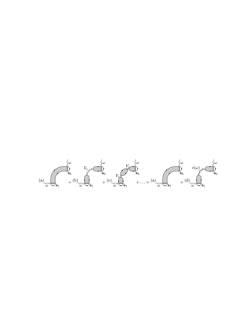
Figure 8: Complete set of diagrams for the bare (without quantum effects) Hall conductivity $\sigma_{xy}^{(0)}(\omega)$ [Eqs. (68)] of the granular system. (a) One starts by connecting the relevant contacts by the intragrain diffusons (see Fig. 6). (b) To get a correct $\omega$-dependence one should take the Coulomb interaction into account by inserting the interaction line into the diffuson. (c) Coulomb interaction, in its turn, is screened by the intragrain motion and one should consider insertions of the polarization bubbles into the interaction line. (d) The summation of the resulting series yields an additional to $\Pi_{xy}^{(0,1)}(\omega)$ [(a), Eq. (61)] contribution $\Pi_{xy}^{(0,2)}(\omega)$ [(d), Eq. (64)] to the current-current correlation function. The sum $\Pi_{xy}^{(0)}(\omega)=\Pi_{xy}^{(0,1)}(\omega)+\Pi_{xy}^{(0,2)}(\omega)$ [Eq. (65)] gives a correct classical expression (68) for the Hall conductivity $\sigma_{xy}^{(0)}(\omega)$.

What is yet missing in our approach? Apparently, one must consider the Coulomb interaction inside the grain. Indeed, the diffuson $D(\omega,{\bf r},{\bf r}^{\prime})$, appearing in Eqs. (57),(61),(62), describes the propagation of electron density, but it does not take into account that electrons are charged and can interact. The correct way to include the classical effect of Coulomb interaction is to insert the interaction line into the diffuson as shown in Fig. 8b. In its turn, this interaction is screened by electron motion, and this can be accounted for by inserting polarization operators into the interaction lines, as shown in Fig. 8c. The summation of the resulting series in Fig. 8 yields the screened form of the Coulomb interaction in a grain $V(\omega,{\bf r},{\bf r}^{\prime})=V(\omega,{\bf i},{\bf i})+v(\omega,{\bf r},{\bf r}^{\prime})$ [Eq. (52)], and we obtain an additional to $\Pi_{\nearrow}^{(0,1)}(\omega)$ [Eq. (55)] contribution

$$\Pi_{\nearrow}^{(0,2)}(\omega)=2g_{T}^{2}\frac{1}{S_{0}^{2}}\int d{\bf s}_{0}d{\bf s}_{1}\int d{\bf r}d{\bf r}^{\prime}\times$$

$$\omega D(\omega,{\bf s}_{0},{\bf r})V(\omega,{\bf r},{\bf r}^{\prime})\omega D(\omega,{\bf r}^{\prime},{\bf s}_{1}).$$

Here the integration with respect to ${\bf r}$ and ${\bf r}^{\prime}$ is done over the grain volume, the spin degeneracy factor 2 comes from an additional electron loop. Due to the orthogonality of the eigenfunctions $\phi_{n}$ [Eq. (41)] the zero modes of $D$ and $V$ drop out of the needed combination

$$\Pi_{xy}^{(0,2)}(\omega)=\Pi_{\nearrow}^{(0,2)}(\omega)+\Pi_{\searrow}^{(0,2)}(\omega)+\Pi_{\swarrow}^{(0,2)}(\omega)+\Pi_{\nwarrow}^{(0,2)}(\omega),$$ (63)

and we get an additional to $\Pi_{xy}^{(0,1)}(\omega)$ [Eq. (61)] contribution (Fig. 8d):

$$\Pi_{xy}^{(0,2)}(\omega)=2\frac{g_{T}^{2}}{\nu}\sum_{n>0}f_{n}\frac{\omega}{\omega+\gamma_{n}}v_{n}(\omega)\frac{\omega}{\omega+\gamma_{n}}$$ (64)

Summing the contributions (61) and (64) we obtain

$$\Pi_{xy}^{(0)}(\omega)\equiv\Pi_{xy}^{(0,1)}(\omega)+\Pi_{xy}^{(0,2)}(\omega)=\frac{g_{T}^{2}}{\nu}\sum_{n>0}\omega f_{n}r_{n},$$ (65)

where

$$r_{n}\equiv\frac{1}{\omega+\gamma_{n}}\left(1+v_{n}(\omega)\frac{2\omega}{\omega+\gamma_{n}}\right)=\frac{1}{\gamma_{n}}$$ (66)

for $\omega\ll\sigma^{\text{gr}}_{xx}$ [see Eq. (49)]. Equations (65) and (66) lead to the final classical expression for the Hall conductivity [Eq. (30)]:

$$\sigma^{(0)}_{xy}(\omega)=2e^{2}a^{2-d}\frac{g_{T}^{2}}{\nu}\sum_{n>0}\frac{f_{n}}{\gamma_{n}},$$ (67)

or, going back to diffusion propagators,

$$\sigma^{(0)}_{xy}(\omega)=2e^{2}a^{2-d}\frac{g_{T}^{2}}{\nu}(\bar{D}_{\nearrow}-\bar{D}_{\searrow}+\bar{D}_{\swarrow}-\bar{D}_{\nwarrow}),$$ (68)

where $\bar{D}_{\alpha}=\frac{1}{S_{0}^{2}}\int d{\bf s}_{0}d{\bf s}_{a}\bar{D}({\bf s}_{0},{\bf s}_{a})$, with $a=1,2,3,4$ for $\alpha=\nearrow,\searrow,\swarrow,\nwarrow$, respectively, and

$$\bar{D}({\bf r},{\bf r}^{\prime})=\sum_{n>0}\frac{\phi_{n}({\bf r})\phi^{*}_{n}({\bf r}^{\prime})}{\gamma_{n}}$$

is the diffuson without the zero mode at $\omega=0$ satisfying Eqs. (38) and (39) with $\omega=0$:

$$-D_{0}\nabla_{\bf r}^{2}\bar{D}({\bf r},{\bf r}^{\prime})=\delta({\bf r}-{\bf r}^{\prime}),$$

$$({\bf n},\nabla_{\bf r}\bar{D})|_{S}=\omega_{H}\tau_{0}({\bf t},\nabla_{\bf r}\bar{D})|_{S}.$$ (69)

It follows from Eqs. (69) that $\bar{D}({\bf r},{\bf r}^{\prime})$ is a Green function for the Poisson equation. Actually the propagator $\bar{D}({\bf r},{\bf r}^{\prime})$ should not be termed “diffuson” anymore, since it describes the propagation of electron density with Coulomb interaction taken into account, i.e. the real conduction process.

Equation (68) constitutes our main result for HC in the absence of quantum effects. We stress that the diagrammatic series in Fig. 8 leading to Eq. (68) describes the classical effect: propagation of electron density in a disordered metallic sample. The temperature-independent result (68) is valid for arbitrary temperature $T$ and arbitrary size $a$ of the grains (not necessarily small grains and $T\ll E_{\text{Th}}$). Temperature will be relevant for quantum effects of Coulomb interaction, which we consider in Sec. VI.

V.1.1 Properties of Eq. (68) for Hall conductivity $\sigma^{(0)}_{xy}$.

Let us discuss the basic properties of Eq. (68). For simplicity, we assume that grains have reflectional symmetry in all three dimensions. Then $\bar{D}_{\nearrow}=\bar{D}_{\swarrow}$ and $\bar{D}_{\searrow}=\bar{D}_{\nwarrow}$ due to this symmetry (for $H\neq 0$, too). At zero magnetic field ($H=0$) we have $\bar{D}_{\nearrow}=\bar{D}_{\searrow}$ and $\bar{D}_{\swarrow}=\bar{D}_{\nwarrow}$ due to the time-reversal symmetry $D(\omega,{\bf r},{\bf r}^{\prime})=D(\omega,{\bf r}^{\prime},{\bf r})$, and therefore $\sigma^{(0)}_{xy}(\omega,H=0)=0$. The nonzero differences $\bar{D}_{\nearrow}-\bar{D}_{\searrow}=\bar{D}_{\swarrow}-\bar{D}_{\nwarrow}$ arise only due to nonzero RHS of the boundary condition Eq. (39), which represents the edge drift. To understand the sign of $\bar{D}_{\nearrow}-\bar{D}_{\searrow}$ and $\bar{D}_{\swarrow}-\bar{D}_{\nwarrow}$ we recall that the diffuson $D(\omega,{\bf r},{\bf r}^{\prime})$ describes the probability of getting from point ${\bf r}^{\prime}$ to point ${\bf r}$. In nonzero field ($H\neq 0$) the edge trajectories for $\bar{D}_{\nearrow}=\bar{D}_{\swarrow}$ are shorter (if $e>0$ is assumed) than those for $\bar{D}_{\searrow}=\bar{D}_{\nwarrow}$, and therefore $\bar{D}_{\nearrow}-\bar{D}_{\searrow}=\bar{D}_{\swarrow}-\bar{D}_{\nwarrow}>0$.

Since $\bar{D}_{\alpha}\propto\frac{1}{a^{3}}\frac{1}{D_{0}a^{-2}}$ and the difference $\bar{D}_{\nearrow}-\bar{D}_{\searrow}$ is linear in $\omega_{H}\tau_{0}$, one can estimate

$$\bar{D}_{\nearrow}-\bar{D}_{\searrow}\propto\frac{1}{a^{3}}\frac{\omega_{H}\tau_{0}}{D_{0}a^{-2}}\propto e^{2}\nu\frac{\rho_{xy}^{\text{gr}}}{a},$$ (70)

where

$$\rho_{xy}^{\text{gr}}=\frac{\sigma_{xy}^{\text{gr}}}{(\sigma_{xx}^{\text{gr}})^{2}}=\frac{\omega_{H}\tau_{0}}{\sigma_{xx}^{\text{gr}}}=\frac{H}{nec}$$

is the specific HR of the grain material expressed in terms of the carrier density $n$ in the grains [Einstein relation $\sigma_{xx}^{\text{gr}}=2e^{2}\nu D_{0}$ was used in Eq. (70)]. We see that $\bar{D}_{\nearrow}-\bar{D}_{\searrow}$ does not depend on the intragrain disorder, described by the scattering time $\tau_{0}$. The proportionality coefficient in Eq. (70) is determined by the shape of the grains only. Thus, for HC [Eq. (68) ] of the system we get

$$\sigma_{xy}^{(0)}\propto a^{2-d}G_{T}^{2}\frac{\rho_{xy}^{\text{gr}}}{a}$$

and for HR [see also Eq. (4)]

$$\rho_{xy}^{(0)}=\frac{\sigma_{xy}^{(0)}}{(\sigma_{xx}^{(0)})^{2}}\propto a^{d-3}\rho_{xy}^{\text{gr}}=a^{d-3}\frac{H}{nec}$$

We come to an important conclusion. The Hall resistivity of the granular system is independent of the intragrain disorder and tunneling conductance. It is expressed solely via the carrier density $n$ of the grain material up to a numerical coefficient determined by the shape of the grains and the type of granular lattice.

V.2 Classical picture

Let us now prove that Eq. (68) for the Hall conductivity indeed reproduces the solution of the classical electrodynamics problem, provided one treats the tunnel contact as a surface resistor with the conductance $G_{T}$.

The classical HC of the granular medium in the limit $G_{T}\ll G_{0}$ [Eq. (3)] can be easily presented in the form of Eq. (5) (see Fig. 1). The current $I_{y}=G_{T}V_{y}$ running through the grain in the $y$ direction causes the Hall voltage drop $V_{H}=R_{H}I_{y}$ between its opposite banks in the $x$ direction, where $R_{H}$ is the Hall resistance of the grain. Since for calculating $\sigma_{xy}$ the total voltage drop per lattice period in the $x$ direction is assumed zero, the same voltage $V_{H}$ (but with the opposite sign) is applied to the contacts in the $x$ direction. Thus, the Hall current equals $I_{x}=G_{T}V_{H}=G_{T}^{2}R_{H}V_{y}$ which leads to the expression (5) for HC.

The Hall resistance $R_{H}$ of the grain is defined via the difference (Hall voltage) of the electric potential $\varphi({\bf r})$ between the opposite banks of the grain in the $x$ direction,

$$V_{H}=\varphi({\bf s}_{r})-\varphi({\bf s}_{l})=R_{H}I_{y},$$ (71)

when the current $I_{y}=I$ passes through the grain in the $y$ direction. The current density

$${\bf j}({\bf r})=-\hat{\sigma}_{0}\nabla_{\bf r}\varphi({\bf r})\equiv-\begin{pmatrix}\sigma_{xx}^{\text{gr}}&\sigma_{xy}^{\text{gr}}&0\\ -\sigma_{xy}^{\text{gr}}&\sigma_{xx}^{\text{gr}}&0\\ 0&0&\sigma_{xx}^{\text{gr}}\\ \end{pmatrix}\nabla_{\bf r}\varphi({\bf r})$$ (72)

($\hat{\sigma}_{0}$ is the conductivity tensor) satisfies the continuity equation

$$\text{div}{\bf j}=q({\bf r})$$ (73)

and the boundary condition

$$({\bf n},{\bf j})|_{S}=0.$$ (74)

The charge source function $q({\bf r})$ is nonzero on the contacts surface only, $\int d{\bf s}_{d}q({\bf s}_{d})=I$ corresponding to the current $I$ flowing into the grain through the contact ${\bf s}_{d}$ and $\int d{\bf s}_{u}q({\bf s}_{u})=-I$ corresponding to the current flowing out of the grain through the contact ${\bf s}_{u}$. The stationary form of Eq. (73) is valid up to the frequencies $\omega\sim\sigma_{xx}^{\text{gr}}$, even if $I=I(t)$ is time-dependent, compare with discussion of Eq. (49) in Sec. IV.2.

Inserting Eq. (72) into Eqs. (73) and (74), we find that $\varphi({\bf r})$ is a solution of the following boundary value problem:

$$-\nabla_{\bf r}^{2}\varphi=q({\bf r})/\sigma_{xx}^{\text{gr}},\mbox{ }({\bf n},\nabla\varphi)|_{S}=\omega_{H}\tau_{0}({\bf t},\nabla\varphi)|_{S}.$$ (75)

Comparing Eq. (75) with Eqs. (69), we see that $\bar{D}({\bf r},{\bf r}^{\prime})$ is a Green function for the problem (75). Thus the solution to Eq. (75) can be written as

$$\varphi({\bf r})=\frac{1}{2e^{2}\nu}\frac{I}{S_{0}}\left(\int d{\bf s}_{d}\bar{D}({\bf r},{\bf s}_{d})-\int d{\bf s}_{u}\bar{D}({\bf r},{\bf s}_{u})\right)$$

(Einstein relation $\sigma_{xx}^{\text{gr}}=2e^{2}\nu D_{0}$ was used). Inserting $\varphi({\bf r})$ in such form into Eq. (71), we obtain for the Hall resistance of the grain:

$$R_{H}=\frac{1}{2e^{2}\nu}(\bar{D}_{\nearrow}-\bar{D}_{\searrow}+\bar{D}_{\swarrow}-\bar{D}_{\nwarrow}),$$ (76)

Comparing Eq. (68) with Eqs. (5) and (76) we see that Eq. (68) indeed reproduces the classical result.

This establishes the correspondence between our diagrammatic approach of considering nonzero diffusion modes and the solution of the classical electrodynamics problem for the granular system.

Luckily, for simple geometries of the grain (cubic, spherical) the Hall resistance $R_{H}$ can be obtained from symmetry arguments without solving the problem Eq. (75). Suppose the grain has reflectional symmetry in all three dimensions. Then it is clear that (1) the largest cross section of the grain lies in the plane of reflection, (2) the current density ${\bf j}({\bf r})$ is perpendicular to the plain of reflection at each point ${\bf r}$ of the cross section, (3) the absolute value of ${\bf j}({\bf r})$ is constant on the cross section and therefore equal to $|{\bf j}({\bf r})|=I/S$, where $S$ is the area of the cross section. So, the Hall voltage Eq. (71) equals $V_{H}=\rho_{xy}^{\text{gr}}|{\bf j}({\bf r})|a=aI/S$. Therefore, the Hall resistance is

$$R_{H}=\rho_{xy}^{\text{gr}}a/S$$ (77)

and the Hall resistivity of the granular medium can be expressed in the form

$$\rho^{(0)}_{xy}=\frac{\sigma^{(0)}_{xy}}{(\sigma^{(0)}_{xx})^{2}}=R_{H}a^{d-2}=\frac{H}{n^{*}ec},$$ (78)

where

$$n^{*}=a^{3-d}An,\mbox{ }A=S/a^{2}\leq 1.$$

The quantity $n^{*}$ defines the effective carrier density of the granular system. For a 3D sample (many grain monolayers), $n^{*}=An$ differs from the actual carrier density $n$ of the grain material only by a numerical factor $A$ determined by the shape of the grains and type of the granular lattice. For a 2D sample $n^{*}=aAn$ for a single grain monolayer or $n^{*}=d_{z}An$ in case of several monolayers, where $d_{z}$ is the thickness of the sample ($d_{z}/a$ is the number of monolayers).

We remind the reader, that Eq. (78) was obtain under the following assumptions: (a) diffusive limit inside the grains, $l\ll a$; (b) the mean free path $l$ is the same for all grains; (c) the tunneling conductance $G_{T}$ is the same for all contacts. Having established the correspondence between our diagrammatic approach and the classical solution of the problem, we can now show that the result (78) is actually valid in a much more general case, when (i) the intragrain disorder is ballistic, $l\gtrsim a$; (ii) the mean free path $l_{\bf i}$ varies from grain to grain (iii) the tunneling conductance $G_{T{\bf i}+{\bf a},{\bf i}}$ varies from contact to contact. The statement (i) follows from the fact that the above classical consideration leading to Eq. (77) involve only the symmetry properties of the current distribution ${\bf j}({\bf r})$ and therefore hold for the grains with ballistic disorder ($l\gtrsim a$) as well. The statement (ii) is true, since the Hall resistance $R_{H}$ [Eq. (77)] of the grain is independent of the mean free path $l_{\bf i}$, and, hence, is the same for all grains ${\bf i}$ provided only their shape is the same. Finally, using the standard Ohm and Kirchhoff laws, we obtain that the Hall voltage between the opposite banks of the sample in the $x$ direction depends on the total Ohmic current flowing through the sample in the $y$ direction. Hence, the Hall voltage is essentially independent of the distribution of the tunneling conductances $G_{T{\bf i}+{\bf a},{\bf i}}$, and the HR of the system is still given by Eq. (78), which proves the statement (iii).

Therefore, the result (78) for Hall resistivity is applicable to real granular systems, in which fluctuations of the intragrain mean free path $l$ and, most importantly, the intergrain tunneling conductance $G_{T}$ are always present.

To conclude this section, we obtain that the classical Hall resistivity [Eq. (78)] of a granular system in the metallic regime, being independent of parameters that describe Ohmic dissipation, possesses a great deal of universality, reminiscent of that in ordinary disordered metals [Eq. (1)].

Being classical, however, Eq. (78) describes the behavior of the Hall resistivity at high enough temperatures, when quantum effects can be neglected. At sufficiently low temperatures quantum effects of Coulomb interaction and weak localization set in and can significantly affect electron transport. In the next section we study quantum corrections to the obtained results (68) and (78) due to the Coulomb interaction between the electrons.

VI Quantum effects of Coulomb interaction

Diagrammatic approach enables us to incorporate quantum effects of Coulomb interaction on the Hall conductivity into the developed scheme. We perform calculations to the first order in the screened Coulomb interaction with the expansion parameter $1/g_{T}$. We assume the diffusive limit for the intragrain dynamics and neglect the diagrams that are small in $\tau_{0}E_{\text{Th}}\propto(l/a)^{2}\ll 1$. The ballistic limit can be treated similarly, although in this case one has to take such diagrams into account.

Technically, one considers the diagrams for the “bare” conductivity $\sigma_{xy}^{(0)}$ shown in Fig. 8 and connects different electron lines by the interaction lines corresponding to the screened Coulomb interaction $V(\Omega,{\bf r}_{\bf i},{\bf r}_{\bf j}^{\prime})$ [Eq. (52)]. It is important that for the quantum interaction corrections the zero-mode part $V(\Omega,{\bf i},{\bf j})$ [Eq. (53)] of the interaction $V(\Omega,{\bf r}_{\bf i},{\bf r}_{\bf j}^{\prime})$ does not drop out and gives a contribution larger than the nonzero intragrain modes $\delta_{{\bf i}{\bf j}}v(\Omega,{\bf r}_{\bf i},{\bf r}^{\prime}_{\bf j})$ [Eq. (49)] (we provide an estimate below). Therefore for the interaction lines that describe the quantum corrections to the classical result we can use the zero-mode part $V(\Omega,{\bf i},{\bf j})$ of the interaction. Further, depending on the sign structure of energies of the Green functions involved, some interaction vertices are renormalized by the diffusons and some are not.

Two types of diagrams can be identified: (i) the interaction $V(\Omega,{\bf i},{\bf j})$ connects different electron loops of the diagrams like in Figs. 9(a),(b); (ii) the interaction $V(\Omega,{\bf i},{\bf j})$ connects points on the same electron loop, like in Figs. 9(c),(d). It is straightforward to show that the former possibility (i) always gives zero: in each case contributing diagrams cancel each other identically , an example is shown in Fig. 9(a),(b). So, we come to an important simplification: electron loops in Fig. 8 are renormalized by the interaction independently.

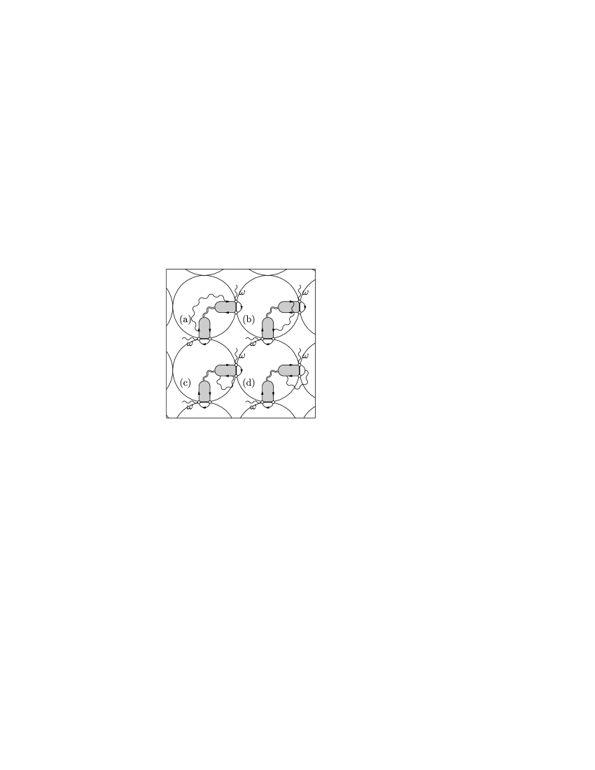
Figure 9: Quantum corrections to Hall conductivity of a granular metal due to Coulomb interaction. Important point: electron loops in diagrams of Fig. 8 are renormalized independently: the diagrams with interaction line connecting different electron loops cancel each other, as is the case, e.g., for the diagrams (a) and (b). Nonvanishing contributions come from the independent renormalization of electron loops by the interaction, like in diagrams (c) and (d).

The temperature $T$, being irrelevant for the single-particle classical transport [Eq. (5) for $\sigma_{xy}^{(0)}$], becomes important for quantum effects of Coulomb interaction. An important energy scale here is the tunneling escape rate $\Gamma$. For $T\gg\Gamma$ the thermal length $L^{*}_{T}=\sqrt{D_{0}^{*}/T}\ll a$ for the intergrain motion ($D_{0}^{*}=\Gamma a^{2}$ is the effective diffusion coefficient) does not exceed the grain size and only the contributions coming from spatial scales of the order of the grain size $a$ are significant. At $T\lesssim\Gamma$ the contributions from the scales $L_{T}^{*}\gtrsim a$ exceeding the grain size also become important.

We start with the former regime $T\gg\Gamma$ in the following subsection. Note that the corrections that will be discussed in Sec. VI.1 are specific to granular systems and absent in HDMs. At the same time they, as we find, govern the $T$-dependence of HC and HR in a wide range of temperatures. The corrections analogous to those in HDMs (“Altshuler-Aronov” corrections) arise from large spatial scales ($\gg a$), are relevant at $T\ll\Gamma$ and will be addressed afterwards in Sec. VI.2, where we consider the case $T\lesssim\Gamma$.

VI.1 “High” temperatures $T\gg\Gamma$

First, we consider the range of temperatures $T\gg\Gamma$ greater than the escape rate $\Gamma$. In this regime each tunneling process brings a small factor $\Gamma/T\ll 1$. Therefore the main contribution comes from the diagrams which contain minimal number of hops between the grains as compared to the diagrams for the bare HC $\sigma_{xy}^{(0)}$. This means that the screened zero-mode interaction can be taken in the form [see Eq. (53)]:

$$V(\Omega,{\bf q})=\frac{E_{c}({\bf q})}{1+2E_{c}({\bf q})\Gamma_{\bf q}/(\delta|\Omega|)}$$ (79)

and for the diffusons renormalizing the interaction vertex we can neglect tunneling completely, i.e., take them as

$$\mathcal{D}(\Omega,{\bf r}_{\bf i},{\bf r}^{\prime}_{\bf j})=\delta_{{\bf i}{\bf j}}D(\Omega,{\bf r}_{\bf i},{\bf r}^{\prime}_{\bf j}).$$

It is very important that, since the interaction $V(\Omega,{\bf i},{\bf j})$ is coordinate-independent within each grain, the intragrain diffusons renormalizing the interaction vertex contain only the zero mode $1/(|\Omega|\mathcal{V})$, whereas the nonzero modes drop out automatically due to the orthogonality condition (41) (we do not simply neglect them):

$$\int d{\bf r}^{\prime}_{\bf i}D(\Omega,{\bf r}_{\bf i},{\bf r}^{\prime}_{\bf i})V(\Omega,{\bf i},{\bf j})=\frac{1}{|\Omega|}V(\Omega,{\bf i},{\bf j}).$$

Assuming $T\gg\Gamma$, we do not assume the temperature $T$ or the frequencies $\Omega$ much smaller than the Thouless energy $E_{\text{Th}}$ in this section. As we will see, the only way to clearly identify the physics of the contributions and obtain a correct upper cut-off for the logarithmically divergent quantities is to include the range $T,\Omega\sim E_{\text{Th}}$ into consideration.

As explained above, we may renormalize electron loops shown in Fig. 8 independently of each other. There are three different types of electron loops in Fig. 8: 1) the (tunneling current)-(tunneling current) correlator $\langle II\rangle$ of the diagram in Fig. 8(a); 2) the (tunneling current)-density correlators $\langle In\rangle$ in Fig. 8(b) connected by the screened interaction $v(\omega,{\bf r},{\bf r}^{\prime})$; 3) the density-density correlators $\langle nn\rangle$ [i.e. the intragrain polarization operator $P(\omega,{\bf r},{\bf r}^{\prime})$, Eq. (47)], in Fig. 8(c), which are the insertions into the bare Coulomb interaction line.

Since the geometry factor $f_{n}$ [Eqs. (59) and (60)] is the same for all diagrams and the properties of the granular array are assumed the same in the $x$ and $y$ directions, let us draw the diagrams in the “longitudinal geometry” (see Figs. 10,12,13). For our purpose it is only important now that there is a “central” grain with a non-zero-mode diffuson and there are two “adjacent” grains. External tunneling vertices are attached to the contacts between the central and adjacent grains.

For each diagram one has to take 4 possibilities (2 for each contact) of attaching external tunneling vertices into account, as in Fig. 6. Only one such possibility is shown in Figs. 10,12,13. Further, for each diagram one has to consider (i) the up/down reversal, if the diagram does not transfer to itself, (ii) the left/right reversal, if the diagram does not transfer to itself. We introduce “up/down reversal” and “left/right reversal” multiplication factors $\alpha^{\text{u/d}}$ and $\alpha^{\text{l/r}}$ correspondingly: $\alpha^{\text{u/d}},\alpha^{\text{l/r}}=1$, if the reversal is not possible, $\alpha^{\text{u/d}},\alpha^{\text{l/r}}=2$, if the reversal is possible.

The summation region over the fermionic frequency $\varepsilon$ of the electron loop and bosonic frequency $\Omega$ carried by the interaction line is determined by the analytical properties of the Green functions involved. After the integration over the Green functions momenta the expressions become independent of $\varepsilon$ and the summation over $\varepsilon$ can be performed. This always results in the sum

$$2\pi T\sum_{\begin{subarray}{c}0<\Omega\leq\omega,\\ -\Omega<\varepsilon<0\end{subarray}}F(\omega,\Omega)+2\pi T\sum_{\begin{subarray}{c}\omega<\Omega,\\ -\omega<\varepsilon<0\end{subarray}}F(\omega,\Omega)=$$

$$=\sum_{0<\Omega\leq\omega}\Omega F(\omega,\Omega)+\omega\sum_{\Omega>\omega}F(\omega,\Omega)=\sum_{\Omega>0}\theta_{\omega,\Omega}F(\omega,\Omega)$$ (80)

standard for the first-order interaction corrections calculations AA . We have introduced the function

$$\theta_{\omega,\Omega}=\left\{\begin{array}[]{ll}\Omega,\mbox{ }&0<\Omega\leq\omega,\\ \omega,\mbox{ }&\Omega>\omega.\end{array}\right.$$

for compactness. The diagrams considered here may contain either one or two summations (80). We introduce the “sum” multiplication factor $\alpha^{\text{s}}$ correspondingly: $\alpha^{\text{s}}=1$ or $\alpha^{\text{s}}=2$. So, each “topologically unique” diagram comes with an overall multiplication factor

$$\alpha=\alpha^{\text{s}}\,\alpha^{\text{u/d}}\alpha^{\text{l/r}}.$$ (81)

We start by considering the corrections to the intragrain polarization operator.

VI.1.1 Corrections to the intragrain polarization operator $P(\omega,{\bf r},{\bf r}^{\prime})$

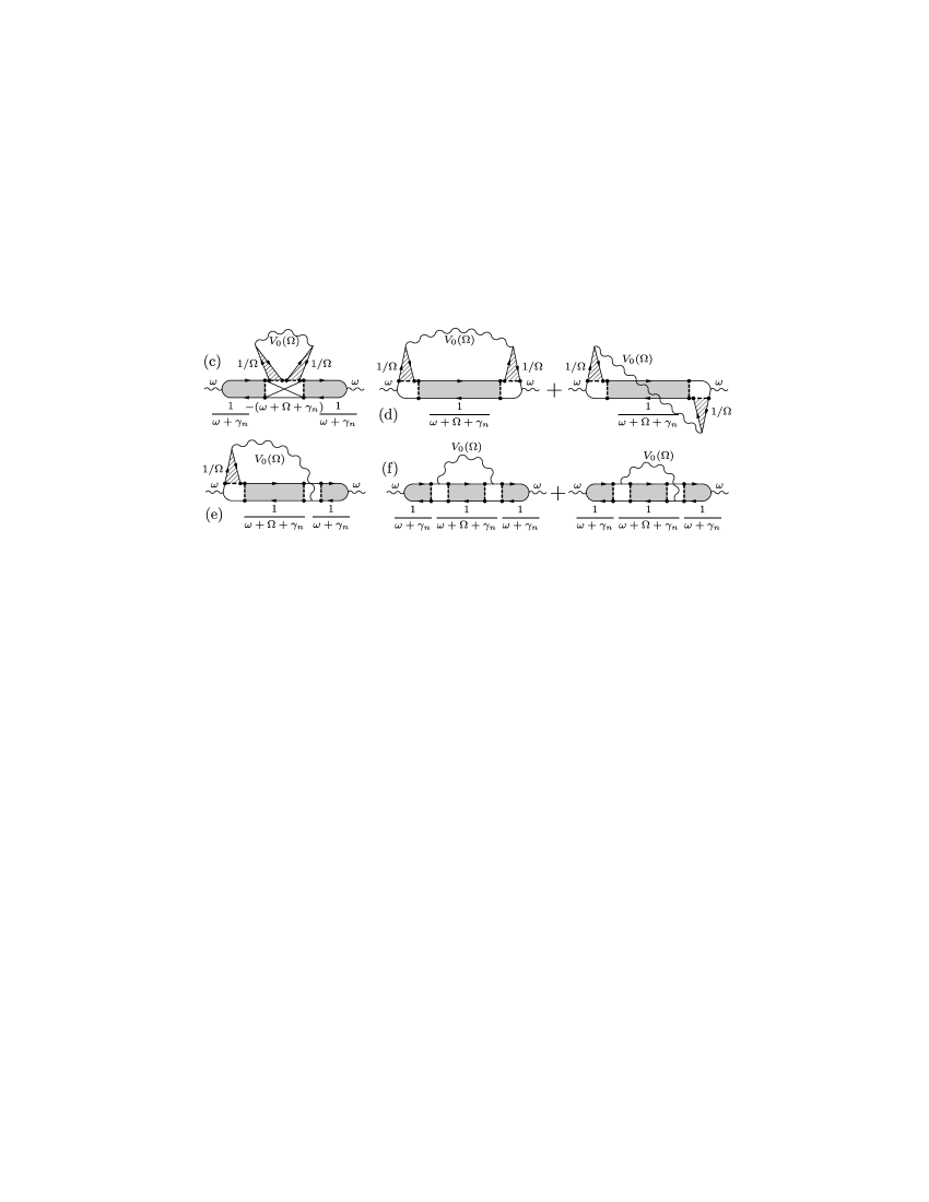
Figure 10: Diagrams for the interaction corrections to the intragrain polarization operator $P_{n}(\omega)=2[1-\omega/(\omega+\gamma_{n})]$ [Eq. (47)]. The corresponding expressions are given in Table 1. Gray blocks depict nonzero diffusion modes, rendered with lines blocks depict zero-mode diffusons $1/\Omega$ renormalizing interaction vertices, dashed lines stand for the impurity correlation function (25). The crossed block in diagram (c) is the Hikami box (see Fig. 11).

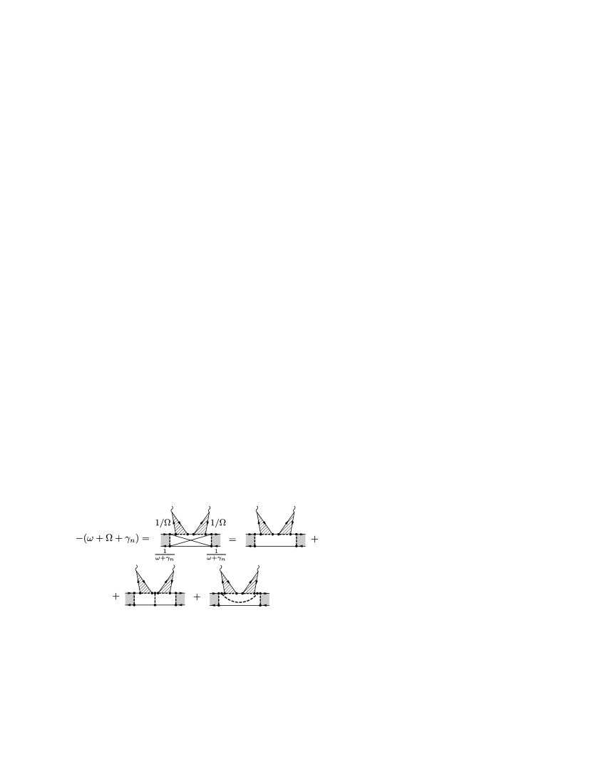
Figure 11: Hikami box. Analytical expression for the Hikami box in case of coordinate-independent interaction potential is $-(\omega+\Omega+\gamma_{n})$.

The set of diagrams for the first-order interaction corrections to the intragrain polarization shown Fig. 10 is the same as the one for a bulk system PO . The crossed region in diagram (c) is a Hikami box HB shown in Fig. 11, which analytical expression for the case of coordinate-independent interaction is $-(\omega+\Omega+\gamma_{n})$.

We present the correction to the $n$-th mode $P_{n}(\omega)=2[1-\omega/(\omega+\gamma_{n})]$ of the polarization operator $P(\omega,{\bf r},{\bf r}^{\prime})$ [Eq. (47)] in the form

$$\delta P^{(i)}_{n}(\omega)=2T\sum_{\Omega>0}\theta_{\omega,\Omega}\,\alpha_{i}\lambda_{n}^{(i)}(\omega,\Omega),\mbox{ }i=\mbox{c,d,e,f},$$ (82)

where the expressions for $\lambda_{n}^{(i)}(\omega,\Omega)$ and the multiplication factors $\alpha_{i}=\alpha_{i}^{\text{s}}\,\alpha_{i}^{\text{u/d}}\alpha_{i}^{\text{l/r}}$ [Eq. (81)] are given in Table 1 (the factor 2 stands for spin degeneracy, the diagrams are labelled in correspondence with the diagrams for $\delta\Pi_{xy}^{(0,1)}(\omega)$ and $\delta\Pi_{xy}^{(0,2)}(\omega)$ below). In Table 1 and Fig. 10, the quantity $V_{0}(\Omega)=V(\Omega,{\bf i},{\bf i})$ is the zero-mode interaction in a given grain. Summing the contributions (82), we obtain that the total correction to the intragrain polarization operator $P_{n}(\omega)$ due to the zero-mode interaction $V_{0}(\Omega)$ vanishes:

$$\delta P^{\text{c}}_{n}(\omega)+\delta P^{\text{d}}_{n}(\omega)+\delta P^{\text{e}}_{n}(\omega)+\delta P^{\text{f}}_{n}(\omega)=0$$ (83)

This is an expected result, since due to the gauge invariance the constant interaction potential cannot affect physical quantities PO ; ZNA , expressed in this case by the density-density correlation function.

$i$	Expression for $\lambda^{(i)}_{n}(\omega,\Omega)$	$\alpha_{i}^{\text{s}}$	$\alpha_{i}^{\text{u/d}}$	$\alpha_{i}^{\text{l/r}}$
c	$\displaystyle-(\omega+\Omega+\gamma_{n})\frac{1}{(\omega+\gamma_{n})^{2}}\frac{1}{\Omega^{2}}V_{0}(\Omega)$	1	2	1
d	$\displaystyle\frac{1}{\omega+\Omega+\gamma_{n}}\frac{1}{\Omega^{2}}V_{0}(\Omega)$	1	2	1
e	$\displaystyle\frac{1}{\omega+\gamma_{n}}\frac{1}{\omega+\Omega+\gamma_{n}}\frac{1}{\Omega}V_{0}(\Omega)$	1	2	2
f	$\displaystyle\frac{1}{(\omega+\gamma_{n})^{2}}\frac{1}{\omega+\Omega+\gamma_{n}}V_{0}(\Omega)$	1	2	1

Table 1: Corrections to the intragrain polarization operator $P_{n}=2[1-\omega/(\omega+\gamma_{n})]$ [Eq. (47)].

As a result, we obtain that the screened non-zero-mode Coulomb interaction $v(\omega,{\bf r},{\bf r}^{\prime})$ [Eq. (49), double wavy line in Fig. 8d] does not acquire any correction. Therefore we should only renormalize the electron loops $\langle II\rangle$ and $\langle In\rangle$ shown in Figs. 8a,d explicitly.

VI.1.2 Interaction corrections to $\Pi_{xy}^{(0,1)}(\omega)$ and $\Pi_{xy}^{(0,2)}(\omega)$.

Now we renormalize the electron loop $\langle II\rangle$ of $\Pi_{xy}^{(0,1)}(\omega)$ [Eq. (61), Fig. 8a)] and two loops $\langle In\rangle$ of $\Pi_{xy}^{(0,2)}(\omega)$ [Eq. (64), Fig. 8d]. The nonzero modes $v_{n}(\omega)$ of the screened intragrain interaction (double wavy line in Fig. 8d) are not renormalized according to the result of the previous subsection.

All corrections to $\Pi_{xy}^{(0,1)}(\omega)$ and $\Pi_{xy}^{(0,2)}(\omega)$ may be presented in the form:

$$\delta\Pi^{(i)}_{xy}(\omega)=\frac{g_{T}^{2}}{\nu}\sum_{n>0}f_{n}\,T\sum_{\Omega>0}\theta_{\omega,\Omega}\,\alpha_{i}\lambda_{n}^{(i)}(\omega,\Omega).$$ (84)

The geometry factor $f_{n}$ [Eqs. (59) and (60)] arises, when corrections to all diagrams in Fig. 6 from the four closest contacts are taken into account. The sets of diagrams giving corrections to $\Pi_{xy}^{(0,1)}(\omega)$ and $\Pi_{xy}^{(0,2)}(\omega)$ are shown in Figs. 12 and 13, and the corresponding expressions for $\lambda_{n}^{(i)}(\omega,\Omega)$ and $\alpha_{i}=\alpha_{i}^{\text{s}}\alpha_{i}^{\text{u/d}}\alpha_{i}^{\text{l/r}}$ are given in Tables 2 and 3, respectively. For each diagram in Figs. 12 and 13 one must take four possibilities [two for each contact according to Eq. (33) and as shown in Fig. 6] of attaching external tunneling vertices into account. In the expressions,

$$V_{0}(\Omega)=V(\Omega,{\bf i},{\bf i})=\sum_{\bf q}V(\Omega,{\bf q})$$

is the “on-cite” interaction of the grain,

$$V_{1}(\Omega)=V(\Omega,{\bf i}+{\bf e}_{i},{\bf i})=\sum_{\bf q}\cos(q_{i}a)V(\Omega,{\bf q}),\mbox{ }i=x,y,$$

is the interaction between the neighboring grains, and

$$V_{2}(\Omega)=V(\Omega,{\bf i}+{\bf e}_{x}+{\bf e}_{y},{\bf i})=\sum_{\bf q}\cos(q_{x}a)\cos(q_{y}a)V(\Omega,{\bf q})$$

is the interaction between the next-to-the-nearest-neighboring grains. The interaction $V(\Omega,{\bf q})$ is given by Eq. (79).

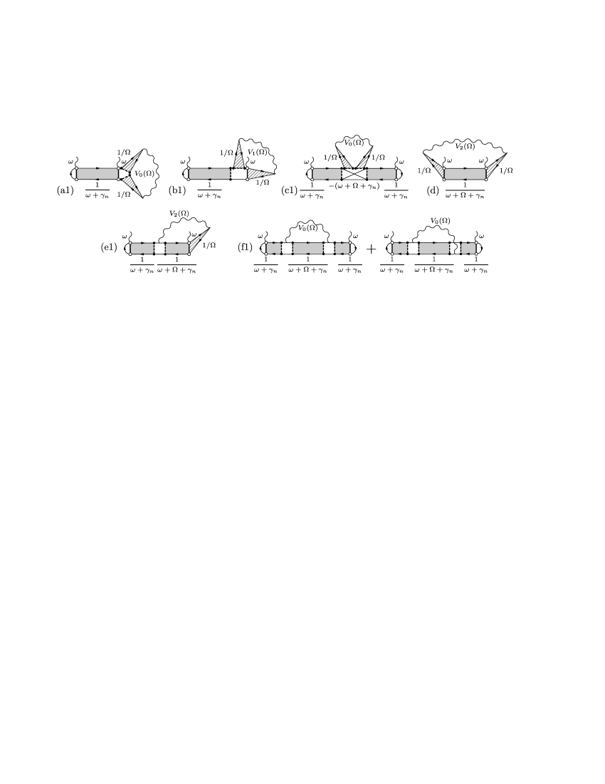
Figure 12: Diagrams for the Coulomb interaction corrections to $\Pi_{xy}^{(0,1)}(\omega)$ [Eq. (61), Fig. 8(a)] describing renormalization of the (tunneling current)-(tunneling current) correlator $\langle II\rangle$ of Fig. 8(a). Open circles denote tunneling vertices placed at the contacts. Other elements are explained in caption to Fig. 10.

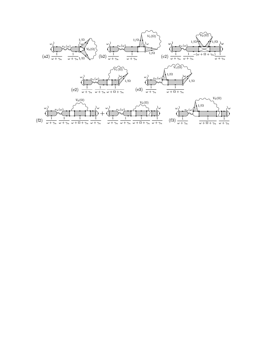
Figure 13: Diagrams for the Coulomb interaction corrections to $\Pi_{xy}^{(0,2)}(\omega)$ [Eq. (64), Fig. 8(d)], describing renormalization of the (tunneling current)-density correlators $\langle In\rangle$ of Fig. 8(d).

$i$	Expression for $\lambda^{(i)}_{n}(\omega,\Omega)$	$\alpha_{i}^{\text{s}}$	$\alpha_{i}^{\text{u/d}}$	$\alpha_{i}^{\text{l/r}}$
a1	$\displaystyle-\frac{1}{\omega+\gamma_{n}}\frac{1}{\Omega^{2}}V_{0}(\Omega)$	2	1	2
b1	$\displaystyle\frac{1}{\omega+\gamma_{n}}\frac{1}{\Omega^{2}}V_{1}(\Omega)$	1	2	2
c1	$\displaystyle-(\omega+\Omega+\gamma_{n})\frac{1}{(\omega+\gamma_{n})^{2}}\frac{1}{\Omega^{2}}V_{0}(\Omega)$	1	2	1
d	$\displaystyle\frac{1}{\omega+\Omega+\gamma_{n}}\frac{1}{\Omega^{2}}V_{2}(\Omega)$	2	1	1
e1	$\displaystyle\frac{1}{\omega+\gamma_{n}}\frac{1}{\omega+\Omega+\gamma_{n}}\frac{1}{\Omega}V_{1}(\Omega)$	1	2	2
f1	$\displaystyle\frac{1}{(\omega+\gamma_{n})^{2}}\frac{1}{\omega+\Omega+\gamma_{n}}V_{0}(\Omega)$	1	2	1

Table 2: Corrections to $\Pi_{xy}^{(0,1)}(\omega)$, [Eq. (61), Fig. 8(a)].

$i$	Expression for $\lambda^{(i)}_{n}(\omega,\Omega)$	$\alpha_{i}^{\text{s}}$	$\alpha_{i}^{\text{u/d}}$	$\alpha_{i}^{\text{l/r}}$
a2	$\displaystyle-\frac{1}{\omega+\gamma_{n}}\frac{1}{\Omega^{2}}V_{0}(\Omega)\left[\frac{2\omega}{\omega+\gamma_{n}}v_{n}\right]$	2	1	2
b2	$\displaystyle\frac{1}{\omega+\gamma_{n}}\frac{1}{\Omega^{2}}V_{1}(\Omega)\left[\frac{2\omega}{\omega+\gamma_{n}}v_{n}\right]$	1	2	2
c2	$\displaystyle-\frac{\omega+\Omega+\gamma_{n}}{(\omega+\gamma_{n})^{2}\Omega^{2}}V_{0}(\Omega)\left[\frac{2\omega}{\omega+\gamma_{n}}v_{n}\right]$	1	2	2
e2	$\displaystyle\frac{1}{\omega+\gamma_{n}}\frac{1}{\omega+\Omega+\gamma_{n}}\frac{1}{\Omega}V_{1}(\Omega)\left[\frac{2\omega}{\omega+\gamma_{n}}v_{n}\right]$	1	2	2
e3	$\displaystyle\frac{1}{\omega+\Omega+\gamma_{n}}\frac{1}{\Omega^{2}}V_{1}(\Omega)\left[\frac{2\omega}{\omega+\gamma_{n}}v_{n}\right]$	1	2	2
f2	$\displaystyle\frac{1}{(\omega+\gamma_{n})^{2}}\frac{1}{\omega+\Omega+\gamma_{n}}V_{0}(\Omega)\left[\frac{2\omega}{\omega+\gamma_{n}}v_{n}\right]$	1	2	2
f3	$\displaystyle\frac{1}{\omega+\gamma_{n}}\frac{1}{\omega+\Omega+\gamma_{n}}\frac{1}{\Omega}V_{0}(\Omega)\left[\frac{2\omega}{\omega+\gamma_{n}}v_{n}\right]$	1	2	2

Table 3: Corrections to $\Pi_{xy}^{(0,2)}(\omega)$, [Eq. (64), Fig. 8(d)].

Note that the diagram (d) in Fig. 12, giving a correction to $\Pi_{xy}^{(0,1)}(\omega)$, does not have an analog for $\Pi_{xy}^{(0,2)}(\omega)$, because this would mean connecting different electron loops by the interaction line, which gives 0, as discussed before. The crossed region in diagrams (c1) and (c2) is the Hikami box (Fig. 11).

Let us perform partial summation of the contributions (84) as follows:

$$\alpha_{\text{a1}}\lambda^{\text{a1}}_{n}(\omega,\Omega)+\alpha_{\text{a2}}\lambda^{\text{a2}}_{n}(\omega,\Omega)=-4\frac{1}{\Omega^{2}}V_{0}(\Omega)r_{n},$$ (85a)

$$\alpha_{\text{b1}}\lambda^{\text{b1}}_{n}(\omega,\Omega)+\alpha_{\text{b2}}\lambda^{\text{b2}}_{n}(\omega,\Omega)=4\frac{1}{\Omega^{2}}V_{1}(\Omega)r_{n},$$ (85b)

$$\sum_{\begin{subarray}{c}i=\text{c1,c2,}\\ \text{f1,f2,f3}\end{subarray}}\alpha_{i}\lambda^{(i)}_{n}(\omega,\Omega)=2\frac{1}{\omega+\Omega+\gamma_{n}}\frac{1}{\Omega^{2}}V_{0}(\Omega)-4\frac{1}{\Omega^{2}}V_{0}(\Omega)r_{n},$$ (85c)

$$\alpha_{\text{d}}\lambda^{\text{d}}_{n}(\omega,\Omega)=2\frac{1}{\omega+\Omega+\gamma_{n}}\frac{1}{\Omega^{2}}V_{2}(\Omega),$$ (85d)

$$\sum_{\begin{subarray}{c}i=\text{e1,}\\ \text{e2,e3}\end{subarray}}\alpha_{i}\lambda^{(i)}_{n}(\omega,\Omega)=4\left[-\frac{1}{\omega+\Omega+\gamma_{n}}\frac{1}{\Omega^{2}}V_{1}(\Omega)+\frac{1}{\Omega^{2}}V_{1}(\Omega)r_{n}\right],$$ (85e)

where $r_{n}=1/\gamma_{n}$ is the “resistance” mode arising as a sum of the series shown in Fig. 8 and given by Eq. (66).

We see that two functionally different forms arise. One contains the frequency-independent resistance modes $r_{n}=1/\gamma_{n}$, the other contains nonzero diffuson modes $1/(\omega+\Omega+\gamma_{n})$. Summing these two independently, we present the total first-order interaction correction $\delta\Pi_{xy}(\omega)$ to the classical result (65) for the current-current correlation function $\Pi_{xy}^{(0)}(\omega)$ as:

$$\delta\Pi_{xy}(\omega)=\delta\Pi^{TA}_{xy}(\omega)+\delta\Pi^{VD}_{xy}(\omega),$$ (86)

where

$$\delta\Pi^{TA}_{xy}(\omega)=-8\frac{g_{T}^{2}}{\nu}\sum_{n>0}f_{n}T\sum_{\Omega>0}\theta_{\omega,\Omega}\,r_{n}\frac{1}{\Omega^{2}}[V_{0}(\Omega)-V_{1}(\Omega)]$$ (87)

and

$$\delta\Pi^{VD}_{xy}(\omega) = 2\frac{g_{T}^{2}}{\nu}\sum_{n>0}f_{n}T\sum_{\Omega>0}\theta_{\omega,\Omega}\,\frac{1}{\omega+\Omega+\gamma_{n}}$$ (88)

$$\times\frac{1}{\Omega^{2}}[V_{2}(\Omega)+V_{0}(\Omega)-2V_{1}(\Omega)].$$

The corresponding correction $\delta\sigma_{xy}(\omega)=\delta\sigma^{TA}_{xy}(\omega)+\delta\sigma^{VD}_{xy}(\omega)$ to Hall conductivity

$$\sigma_{xy}(\omega)=\sigma^{(0)}_{xy}+\delta\sigma_{xy}(\omega),$$ (89)

is obtained from Eq. (86) according to Eq. (30):

$$\delta\sigma_{xy}(\omega)=2e^{2}a^{2-d}\frac{1}{\omega}\delta\Pi_{xy}(\omega)$$ (90)

Let us discuss the obtained results (86),(87),(88). First of all, note that the corrections $\delta\Pi^{TA}_{xy}(\omega)$ and $\delta\Pi^{VD}_{xy}(\omega)$ cannot be attributed to certain separate sets of diagrams: the diagrams (a1),(a2),(b1),(b2) contribute to $\delta\Pi^{TA}_{xy}(\omega)$ only [Eqs. (85a) and (85b)], the diagram (d) contributes to $\delta\Pi^{VD}_{xy}(\omega)$ only [Eq. (85d)], but the rest of the diagrams contain parts corresponding both to $\delta\Pi^{TA}_{xy}(\omega)$ and $\delta\Pi^{VD}_{xy}(\omega)$, as seen from Eqs. (85c) and (85e)

Note also that the corrections $\delta\Pi^{TA}_{xy}(\omega)$ and $\delta\Pi^{VD}_{xy}(\omega)$ vanish separately in the case of constant interaction potential, i.e., when $V_{0}(\Omega)=V_{1}(\Omega)=V_{2}(\Omega)$. This property is not accidental and is enforced by the gauge invariance (see, e.g., Refs. PO, ; ZNA, ): constant interaction potential results in a shift of the chemical potential of the whole electron system and therefore does not affect physical quantities expressed diagrammatically as chains of closed electron loops (see Fig. 8). This fact serves as an important check of our results (86),(87), and (88). We remind the reader that Eq. (83) is also a consequence of the gauge invariance.

The physical processes leading to the corrections $\delta\Pi^{TA}_{xy}(\omega)$ and $\delta\Pi^{VD}_{xy}(\omega)$ are most clearly identified from the diagrams that contribute to either one of the quantities, i.e., from the diagrams (a1),(a2),(b1),(b2) for $\delta\Pi^{TA}_{xy}(\omega)$ and from the diagram (d) for $\delta\Pi^{VD}_{xy}(\omega)$.

VI.1.3 “Tunneling anomaly” contribution $\delta\Pi^{TA}_{xy}(\omega)$

First, consider the correction $\delta\Pi^{TA}_{xy}(\omega)$ [Eq. (87)]. Clearly, the diagrams (a1),(a2),(b1),(b2), contributing solely to $\delta\Pi^{TA}_{xy}(\omega)$, describe the effect of Coulomb interaction on the process of electron tunneling through the contact. Therefore, the correction $\delta\Pi^{TA}_{xy}(\omega)$ should be attributed to the tunneling anomalyAA ; TA1 ; TA2 (TA) effect in a granular metal. The correction $\delta\Pi^{TA}_{xy}(\omega)$ corresponds to the independent renormalization of the tunneling conductances $G_{T}$ of the individual contacts in formula (5) for the bare classical HC $\sigma_{xy}^{(0)}\propto G_{T}^{2}R_{H}$, whereas the Hall resistance $R_{H}$ of the grain remains unaffected.

Indeed, the $\Omega$-independent resistance modes $r_{n}$ [Eq. (66)] can be taken out of the sum over $\Omega$ in Eq. (87). After that the summed over $\Omega$ expression becomes independent of the mode index $n$ and we can reduce the relative correction to the current-current correlation function and HC to the form:

$$\frac{\delta\sigma^{TA}_{xy}(\omega)}{\sigma^{(0)}_{xy}}=\frac{\delta\Pi^{TA}_{xy}(\omega)}{\Pi^{(0)}_{xy}(\omega)}=2\frac{\delta g_{T}(\omega)}{g_{T}},$$ (91)

where we have introduced the quantity

$$\frac{\delta g_{T}(\omega)}{g_{T}}=-\frac{1}{\omega}4T\sum_{\Omega>0}\theta_{\omega,\Omega}\frac{1}{\Omega^{2}}[V_{0}(\Omega)-V_{1}(\Omega)].$$ (92)

The expression in the RHS of Eq. (92) should be treated as a relative correction to the tunneling conductance $g_{T}$ of the individual contact due to the tunneling anomaly. [The factor 2 in Eq. (91) stands for two contacts according to the square $G_{T}^{2}$ in Eq. (5) for $\sigma_{xy}^{(0)}$.] Such physical interpretation most clearly arises from the calculations of interaction corrections to LC. The bare LC $\sigma_{xx}^{(0)}\propto g_{T}$ [Eq. (4)] (in the lowest in $g_{T}/g_{0}\ll 1$ order) is expressed solely via the tunneling conductance $g_{T}$ and the interaction correction to $\sigma_{xx}^{(0)}$ corresponds to the renormalization of $g_{T}$, since no other physical parameters are available. The interaction corrections to LC $\sigma_{xx}^{(0)}$ were studied in Refs. ET, ; BELV, and at $T\gg\Gamma$ the correction $\delta\sigma_{xx}^{TA}(\omega)$ to LC

$$\sigma_{xx}(\omega)=\sigma_{xx}^{(0)}+\delta\sigma_{xx}^{TA}(\omega)$$ (93)

was obtained:

$$\frac{\delta\sigma^{TA}_{xx}(\omega)}{\sigma^{(0)}_{xx}}=\frac{\delta g_{T}(\omega)}{g_{T}}.$$ (94)

Therefore, according to the form of Eq. (91), the correction $\delta\Pi^{TA}_{xy}(\omega)$ indeed corresponds to the renormalization of the tunnelling conductances $G_{T}$ in Eq. (5) and does not affect the Hall resistance $R_{H}$ of the grain.

VI.1.4 Virtual diffusion contribution $\delta\Pi^{VD}_{xy}(\omega)$

Now let us discuss the correction $\delta\Pi^{VD}_{xy}(\omega)$ [Eq. (88)]. The diagram (d), which contributes solely to $\delta\Pi^{VD}_{xy}(\omega)$, describes electron diffusion through the central grain. The corresponding diffuson $D(\omega+\Omega,{\bf r},{\bf r}^{\prime})$ enters Eq. (88) as the combination

$$\sum_{n>0}\frac{f_{n}}{\omega+\Omega+\gamma_{n}} = D_{\nearrow}(\omega+\Omega)-D_{\searrow}(\omega+\Omega)$$

$$+D_{\swarrow}(\omega+\Omega)-D_{\nwarrow}(\omega+\Omega)$$

[see Eqs. (58) and (59)] and therefore contains nonzero modes $n>0$ only.

As discussed above, one cannot “construct” the propagator $\bar{D}({\bf r},{\bf r}^{\prime})$ [see Eqs. (69),(66)], which describes the real propagation of electron density in metals (basically, the classical conduction process), from the diffuson $D(\omega+\Omega,{\bf r},{\bf r}^{\prime})$ by inserting interaction lines into the central diffuson in the diagram (d): the corresponding diagrams simply cancel each other. This emphasizes virtual character of the diffusion: real diffusion is not possible in metallic samples, since nonequilibrium electron density created in the course of diffusion is screened by Coulomb interaction.

Thus, the correction $\delta\Pi^{VD}_{xy}(\omega)$ describes the process of “virtual diffusion” (VD) of electrons through the grain.

VI.1.5 Why $\Omega,T\sim E_{\text{Th}}$ are necessary

We emphasize that it has become possible to identify two physically different contributions $\delta\Pi^{TA}_{xy}(\omega)$ [Eq. (87)] and $\delta\Pi^{VD}_{xy}(\omega)$ [Eq. (88)] to the total correction $\delta\Pi_{xy}(\omega)$ [Eq. (86)] only because we have included “high” frequency range $\Omega\sim E_{\text{Th}}$ in our calculations. At frequencies $\Omega\ll E_{\text{Th}}$ the expressions in Eqs. (87) and (88) acquire the same functional form, since $1/(\omega+\Omega+\gamma_{n})\approx 1/\gamma_{n}=r_{n}$ and one cannot distinguish between them.

Including the frequencies $\Omega\sim E_{\text{Th}}$ has complicated the calculations significantly. Indeed, for $\Omega\ll E_{\text{Th}}$ one may consider the diagrams (a1),(b1),(c1),(d) only. The rest of the diagrams are smaller than these ones in $\Omega/E_{\text{Th}}\ll 1$ or $\omega/E_{\text{Th}}\ll 1$ and become comparable to them only at $\Omega,\omega\sim E_{\text{Th}}$. Considering the diagrams (a1),(b1),(c1),(d) only and neglecting the frequencies $\omega,\Omega$ compared to $\gamma_{n}\gtrsim E_{\text{Th}}$ in the diffusons $1/(\omega+\gamma_{n})$ and $1/(\omega+\Omega+\gamma_{n})$, we would get the total correction $\delta\Pi_{xy}(\omega)$ [Eq. (86)] in the form

$$\delta\Pi_{xy}(\omega) = -2\frac{g_{T}^{2}}{\nu}\sum_{n>0}f_{n}T\sum_{\Omega>0}\theta_{\omega,\Omega}\,\frac{1}{\gamma_{n}}\frac{1}{\Omega^{2}}\times$$ (95)

$$\times [3V_{0}(\Omega)-2V_{1}(\Omega)-V_{2}(\Omega)],$$

which is just the sum of $\delta\Pi^{TA}_{xy}(\omega)$ and $\delta\Pi^{VD}_{xy}(\omega)$ provided one neglects $\omega+\Omega$ in $1/(\omega+\Omega+\gamma_{n})$. Clearly, the above physical analysis would not be possible based on the form of Eq. (95).

Another related drawback of considering small frequencies $\Omega\ll E_{\text{Th}}$ only will be clear in the next subsection, where we turn to the temperature dependence of the obtained corrections.

VI.1.6 Temperature dependence of the corrections

Now let us discuss what consequences the corrections (86),(87),(88) have on the Hall conductivity $\sigma_{xy}(\omega)$ and, more importantly, on the Hall resistivity

$$\rho_{xy}(\omega)=\frac{\sigma_{xy}(\omega)}{\sigma_{xx}^{2}(\omega)}=\rho_{xy}^{(0)}+\delta\rho_{xy}(\omega),$$

which is directly measurable experimentally. The conductivities $\sigma_{xy}(\omega)$ and $\sigma_{xx}(\omega)$ are given by Eqs. (89) and (93), respectively, and the “bare” HR $\rho_{xy}^{(0)}$ by Eq. (78).

First of all, since $\rho_{xy}^{(0)}$ [Eq. (78)] simply does not contain $G_{T}$, the tunneling anomaly effect does not influence the Hall resistivity. Indeed, according to Eqs. (91) and (94), we obtain that the correction to HR due to TA vanishes:

$$\frac{\delta\rho_{xy}^{TA}(\omega)}{\rho_{xy}^{(0)}}=\frac{\delta\sigma^{TA}_{xy}(\omega)}{\sigma^{(0)}_{xy}}-2\frac{\delta\sigma^{TA}_{xx}(\omega)}{\sigma^{(0)}_{xx}}\equiv 0.$$

Next, since the analog of VD correction (88) is absent for LC $\sigma_{xx}(\omega)$ [see Eq. (93)] in the leading in $g_{T}/g_{0}\ll 1$ order , the correction to Hall resistivity due to virtual diffusion process is

$$\frac{\delta\rho_{xy}^{VD}(\omega)}{\rho_{xy}^{(0)}}=\frac{\delta\sigma_{xy}^{VD}(\omega)}{\sigma_{xy}^{(0)}}=\frac{\delta\Pi^{VD}_{xy}(\omega)}{\Pi^{(0)}_{xy}(\omega)}.$$

Therefore, we obtain that the total correction

$$\delta\rho_{xy}(\omega)=\delta\rho_{xy}^{TA}(\omega)+\delta\rho_{xy}^{VD}(\omega)$$

to HR at temperatures $T\gg\Gamma$ is due to VD effect only:

$$\frac{\delta\rho_{xy}(\omega)}{\rho_{xy}^{(0)}}=\frac{\delta\sigma_{xy}^{VD}(\omega)}{\sigma_{xy}^{(0)}}.$$

Now, let us discuss the temperature dependence of the obtained corrections. The Coulomb potential (79) is completely screened and equal to the inverse polarization operator,

$$V(\Omega,{\bf q})=\frac{\delta}{\mathcal{P}_{0}(\Omega,{\bf q})}=\frac{\delta\,\Omega}{2\Gamma_{\bf q}},$$

for frequencies $\Omega\lesssim g_{T}E_{c}$. In the limit of high frequencies $\Omega\gtrsim g_{T}E_{c}$ the Coulomb potential (79) remains unscreened and $V(\Omega,{\bf q})\sim E_{c}$. The expression

$$\frac{1}{\Omega^{2}}V(\Omega,{\bf q})=\frac{1}{\Omega}\frac{\delta}{2\Gamma_{\bf q}}$$ (96)

in Eqs. (87) and (88) is thus proportional to $1/\Omega$ for $\Omega\lesssim g_{T}E_{c}$. Therefore, the sum of over $\Omega$ is logarithmically divergent and we have to determine the low and high frequency cut-offs.

In the d.c. limit $\omega\ll T$, the low frequency cut-off for the sum over $\Omega$ is set by the temperature $T$ (for $T\gg\Gamma$). This can be obtained by the analytical continuation of Eqs. (87) and (88) to real frequencies $\omega$ and taking the limit $\omega\ll T$ according to

$$T\sum_{\Omega_{m}>0}\theta_{\omega_{n},\Omega_{m}}F(i\Omega_{m})|_{i\omega_{n}\rightarrow\omega+i0,\omega\ll T}=$$

$$=-\frac{\omega}{4\pi}\int_{-\infty}^{\infty}d\varepsilon\frac{d}{d\varepsilon}\left(\varepsilon\coth\frac{\varepsilon}{2T}\right)F(\varepsilon),$$

we do not repeat this standard procedure here (see, e.g., Refs. AAjetp, ; ZNA, , the integer indices of the Matsubara frequencies $\omega_{n}$ and $\Omega_{m}$ were written for clarity).

The high-frequency cut-off is different for TA contribution $\delta\Pi_{xy}^{TA}$ and VD contribution $\delta\Pi_{xy}^{VD}$, which is a direct consequence of their different physical origin. According to Eq. (92) the upper cut-off for $\delta\Pi_{xy}^{TA}$ is $g_{T}E_{c}$. At $\Omega\gtrsim g_{T}E_{c}$ we have $V(\Omega)/\Omega^{2}\sim E_{c}/\Omega^{2}$ and the sum converges. Therefore, the correction (92) to the tunneling conductance $g_{T}$ takes the formET ; BELV

$$\frac{\delta g_{T}(T)}{g_{T}}=-\frac{1}{2\pi g_{T}d}\ln\frac{g_{T}E_{c}}{T}$$ (97)

and for the TA correction to HC from Eqs. (87) and (91) we get:

$$\frac{\delta\sigma_{xy}^{TA}(T)}{\sigma_{xy}^{(0)}}=-\frac{1}{\pi g_{T}d}\ln\frac{g_{T}E_{c}}{T}.$$ (98)

The lattice-specific factor $1/d$ arises as an integral

$$\frac{1}{d}=\int\frac{a^{d}d^{d}{\bf q}}{(2\pi)^{d}}\frac{1-\cos q_{x}a}{\sum_{\beta}(1-\cos q_{\beta}a)}.$$ (99)

For the VD contribution $\delta\Pi_{xy}^{VD}$ the summed over $\Omega$ expression contains additional $\Omega$ in the denominator coming from the intragrain nonzero diffusion mode $1/(\omega+\Omega+\gamma_{n})$. Therefore, the expression is proportional to $1/\Omega$ provided not only $\Omega\lesssim g_{T}E_{c}$, but also $\Omega\lesssim E_{\text{Th}}$. Thus, the upper cut-off is the minimum of the two quantities, i.e., $\min(E_{\text{Th}},g_{T}E_{c})$. Calculating the sum in Eq. (88) and extracting $\sigma^{(0)}_{xy}$ with the help of Eq. (68), we get

$$\frac{\delta\sigma^{VD}_{xy}(T)}{\sigma^{(0)}_{xy}}=\frac{c_{d}}{4\pi g_{T}}\ln\left[\frac{\min(g_{T}E_{c},E_{\text{Th}})}{T}\right],$$ (100)

where

$$c_{d}=\int\frac{a^{d}d^{d}{\bf q}}{(2\pi)^{d}}\frac{(1-\cos q_{x}a)(1-\cos q_{y}a)}{\sum_{\beta}(1-\cos q_{\beta}a)}$$ (101)

is the lattice form-factor. Appearance of the Thouless energy $E_{\text{Th}}$ as an additional cut-off in Eq. (100) reflects the diffusive nature of the contribution. Virtual diffusion process is suppressed for $T\gtrsim E_{\text{Th}}$, since in this case the intragrain thermal length $L_{T}=\sqrt{D_{0}/T}\lesssim a$ becomes smaller than the size $a$ of the grain.

We conclude that, the total correction to HR at temperatures $T\gg\Gamma$ is due to virtual diffusion process only and equals

$$\frac{\delta\rho_{xy}(T)}{\rho^{(0)}_{xy}}=\frac{\delta\sigma^{VD}_{xy}(T)}{\sigma^{(0)}_{xy}}=\frac{c_{d}}{4\pi g_{T}}\ln\left[\frac{\min(g_{T}E_{c},E_{\text{Th}})}{T}\right].$$ (102)

We see that due to the logarithmic divergence of the corrections (98) and (100) one is forced to go to the frequencies $\Omega\sim E_{\text{Th}}$ in order to get a correct upper cut-off, even if one considers the temperatures $T\ll E_{\text{Th}}$. This has direct consequences on physical quantities. The upper cut-off also determines the upper bound for the temperature range, in which the corrections have the $\ln T$-dependence of Eqs. (98) and (100). So, HR $\rho_{xy}(T)=\rho_{xy}^{(0)}+\delta\rho_{xy}(T)$ is $\ln T$-dependent according to Eq. (102) for $\Gamma\lesssim T\lesssim\min(g_{T}E_{c},E_{\text{Th}})$, whereas LR $\rho_{xx}(T)=1/\sigma_{xx}(T)$ is $\ln T$-dependent according to Eq. (97) for $\Gamma\lesssim T\lesssim g_{T}E_{c}$. For $T\gtrsim\min(g_{T}E_{c},E_{\text{Th}})$ the relative correction to HR $\delta\rho_{xy}(T)/\rho^{(0)}_{xy}\lesssim 1/g_{T}$ becomes insignificant. The ratio of $g_{T}E_{c}$ and $E_{\text{Th}}$ can be arbitrary in a real system. In case $E_{\text{Th}}\ll g_{T}E_{c}$ HR $\rho_{xy}(T)$ is $\ln T$-dependent in a narrower range $\Gamma\lesssim T\lesssim E_{\text{Th}}$ than LR $\rho_{xx}(T)$. We emphasize, that perturbative approach used by us is applicable as long as the relative correction (102) is small.

Note that the integrals over ${\bf q}$ in Eqs. (99) and (101) do not diverge at small $qa\ll 1$, although $\Gamma_{\bf q}=2\Gamma\sum_{\beta}(1-\cos q_{\beta}a)\rightarrow 0$ as $qa\rightarrow 0$. This is a consequence of the gauge-invariance mentioned previously. At the same time, this is not the case for the density of statesET .

The lattice factors $1/d$ and $c_{d}$ in Eqs. (98),(100),(102) are not universal and are specific for quadratic/cubic lattice we considered. However the $\ln T$-dependence itself is a result of the screened form of the Coulomb interaction in granular metals and is robust to the lattice structure. For a different type of lattice the logarithmic dependence of Eqs. (98),(100),(102) remains the same, although numerical prefactors may be different.

Moreover, we expect the logarithmic form of Eqs. (98),(100),(102) to persist even if one allow for fluctuations (at least, moderate) of tunneling conductances $G_{T}$ from contact to contact. The reason is that the logarithmic contribution arises from the integration over frequency: $\int^{g_{T}E_{c}}_{T}d\Omega/\Omega=\ln(g_{T}E_{c}/T)$, which is “decoupled” from the integration over quasimomentum ${\bf q}$ in Eqs. (87),(88) [see Eq. (96)] in the considered range of $\Omega$. The tunneling conductance $g_{T}$ enters as an upper cutoff, which precise value with logarithmic accuracy is not important. So, for a realistic array with randomly distributed tunneling condcutances the form of Eqs. (98),(100),(102) should remain, although the lattice structure factors $1/d$ and $c_{d}$ should be replaced by some other distribution-dependent factors of the order of unity and $g_{T}$ by some distribution-averaged value.

We mention in this respect that the logarithmic renormalization of individual conductances for an array with randomly distributed tunneling conductances was studied by Feigelman, Ioselevich, and Skvortsov in Ref. FIS, and, indeed, it was shown that the $\ln T$-dependence of Eq. (97) for the effective tunneling conductance persists.

VI.1.7 Estimate for the contribution from nonzero interaction modes.

As we claimed above, coordinate-dependent intragrain interaction modes $\delta_{{\bf i}{\bf j}}v(\Omega,{\bf r}_{\bf i},{\bf r}^{\prime}_{\bf j})$ [Eq. (49)] of the screened potential $V(\Omega,{\bf r}_{\bf i},{\bf r}^{\prime}_{\bf j})$ [Eq. (52)] give a smaller contribution than the zero-mode part $V(\Omega,{\bf i},{\bf j})$ [Eq. (53)] in the relevant range $\Omega,T\lesssim E_{\text{Th}}$. We provide an estimate here.

Let us revise, for example, the diagrams (a1),(a2) in Figs. 12 and 13 taking now nonzero modes of the screened interaction into account. For the block in the right grain, we have

$$T\sum_{\Omega>0}\int d{\bf r}\,d{\bf r}^{\prime}D(\Omega,{\bf s},{\bf r})V(\Omega,{\bf r},{\bf r}^{\prime})D(\Omega,{\bf r}^{\prime},{\bf s})=$$

$$=T\sum_{\Omega>0}\left[\frac{1}{\Omega^{2}}V_{0}(\Omega)+\sum_{n>0}\frac{|\phi_{n}({\bf s})|^{2}}{(\Omega+\gamma_{n})^{2}}\frac{1}{\nu}v_{n}(\Omega)\right]$$

The first term in the RHS is the contribution from the zero-mode interaction $V_{0}(\Omega)$ we had before, whereas the second one is the contribution from nonzero modes $v_{n}(\Omega)$, which we want to estimate now (${\bf s}$ is a point on the contact). Since $V_{0}(\Omega)\sim\delta\Omega/\Gamma$ for $\Omega\lesssim g_{T}E_{c}$, the first term gives the logarithmic contribution (97) to the conductivity:

$$T\sum_{\Omega>0}\frac{1}{\Omega^{2}}V_{0}(\Omega)\sim\frac{1}{g_{T}}\ln\frac{g_{T}E_{c}}{T}$$ (103)

As $v_{n}(\Omega)\sim(\Omega+\gamma_{n})/\gamma_{n}$ for $\Omega\lesssim\min(1/\tau_{0},\sigma^{\text{gr}}_{xx})=1/\tau_{0}$, the contribution from nonzero modes is estimated as

$$T\sum_{\Omega>0}\delta\sum_{n>0}\frac{1}{\Omega+\gamma_{n}}\frac{1}{\gamma_{n}}\sim\frac{1}{\nu D_{0}}\int_{T}^{\infty}d\Omega\int_{1/a}^{\infty}\frac{dq}{\Omega+D_{0}q^{2}}\sim$$

$$\sim\frac{1}{(p_{F}l)^{2}}[1-\alpha\sqrt{\tau_{0}\max(T,E_{\text{Th}})}]$$ (104)

(here $\alpha\sim 1$ is a cutoff-dependent number). The obtained contribution from nonzero modes is nothing else but the tunneling anomaly in 3D case AAssc1 ; AAjetp ; AAssc2 (since the grains are three-dimensional), the square root describing well-known singularity. We see, that the contribution (104) from nonzero modes is smaller than the contribution (103) from zero modes if the condition

$$g_{0}/g_{T}\gg a/l$$ (105)

is met. Since $g_{0}\gg g_{T}$ [Eq. (3)], for ballistic grains ($l\sim a$) this is always the case. More important, however, is that in the relevant temperature range $T\lesssim E_{\text{Th}}$ the contribution (104) is $T$-independent. Therefore, even if the condition (105) is not well met, nonzero modes give an inessential $T$-independent renormalization of the bare quantities for $T\lesssim E_{\text{Th}}$ not affecting the overall $T$-dependence of the HC and HR in that range.

VI.2 “Low” temperatures $T\lesssim\Gamma$

Now we want to include the region of temperatures $T\lesssim\Gamma$ of the order or smaller than the escape rate $\Gamma$ into our considerations. In this regime the thermal length for the intergrain motion $L_{T}^{*}=\sqrt{\Gamma a^{2}/T}\gtrsim a$ is greater than the size of the grain $a$ and quantum phenomena can occur not only inside the grains, but also at spatial scales much exceeding the grain size.

The technical complication in considering $T\lesssim\Gamma$ instead of $T\gg\Gamma$ is that we have to take tunneling fully into account. At the same time we still have a small parameter $\Gamma/E_{\text{Th}}\ll 1$ [Eq. (2)], which allows us to neglect nonzero intragrain modes compared to the zero modes as long as we consider the frequencies $\Omega\ll E_{\text{Th}}$.

As we have discussed in the previous section, even for temperatures $T\ll E_{\text{Th}}$ considering $\Omega\sim E_{\text{Th}}$ in the expression

$$\delta\Pi_{xy}(\omega)=\sum_{\Omega>0}\theta_{\omega,\Omega}F(\Omega)$$

for the correction to HC is necessary in order to obtain a correct upper cut-off for logarithmically the diverging quantities. At the same time for $\Omega\sim E_{\text{Th}}$ the results must match with those of the previous section, since for $\Omega\gg\Gamma$ one can neglect tunneling in the expressions.

Therefore, to simplify our calculations we do assume $\Omega\ll E_{\text{Th}}$ in this section. Having obtained the results limited by $\Omega\ll E_{\text{Th}}$, we determine the upper cut-off by matching them with the results of the previous section in the range $\Gamma\ll\Omega\ll E_{\text{Th}}$, where both results are applicable.

The diagrams for $T\lesssim\Gamma$ can be obtained from the diagrams in Figs. 12 and 13 for $T\gg\Gamma$ by including higher orders in tunneling. As we restrict ourselves to low frequencies $\Omega\ll E_{\text{Th}}$, only four diagrams (a1),(b1),(c1),(d) should be considered and the rest of the diagrams are smaller in $\Omega/E_{\text{Th}}\ll 1$. Taking tunneling into account we make sure that in each diagram only one grain contains nonzero diffusion modes necessary to have a nonvanishing contribution to the Hall current, whereas in the rest of the grains only the zero mode is retained. The zero-mode interaction potential $V(\Omega,{\bf i},{\bf j})$ is now taken in the form (53). Considering the range $\omega,\Omega\ll E_{\text{Th}}$, we also neglect the frequency dependence of nonzero modes now: $1/(\omega+\Omega+\gamma_{n})=1/\gamma_{n}$ and $1/(\omega+\gamma_{n})=1/\gamma_{n}$.

VI.2.1 Short-scale contribution

Including higher orders in tunneling in diagrams (a1), (b1), and (c1) in Fig. 12 is straightforward. One has to substitute the zero-mode diffusons $\delta_{{\bf i}{\bf j}}/\Omega$ renormalizing the interaction vertices by their form $\mathcal{D}_{0}(\Omega,{\bf i},{\bf j})$ [Eq. (51)], which takes tunneling into account:

$$\delta_{{\bf i}{\bf j}}\frac{1}{\Omega}\rightarrow\mathcal{D}_{0}(\Omega,{\bf i},{\bf j}),\mbox{ }\mathcal{D}_{0}(\Omega,{\bf q})=\frac{1}{\Omega+\Gamma_{\bf q}}.$$

This results in the replacement of $V(\Omega,{\bf i},{\bf j})/\Omega^{2}$ in the expressions for $\lambda^{(i)}_{n}(\omega,\Omega)$, $i=\text{a1},\text{b1},\text{c1}$, (see Table 2) by

$$\widetilde{V}(\Omega,{\bf i},{\bf j})=\sum_{{\bf k},{\bf l}}\mathcal{D}_{0}(\Omega,{\bf i},{\bf k})V(\Omega,{\bf k},{\bf l})\mathcal{D}_{0}(\Omega,{\bf l},{\bf j}),$$

$$\widetilde{V}(\Omega,{\bf q})=\mathcal{D}_{0}^{2}(\Omega,{\bf q})V(\Omega,{\bf q}).$$

Consequently, instead of Eqs. (85a), (85b), and (85c) we get [Fig. 14(a),(b),(c)]

$$\alpha_{\text{a}}\lambda^{\text{a}}_{n}(\omega,\Omega)=-4\widetilde{V}_{0}(\Omega)\frac{1}{\gamma_{n}},$$ (106a)

$$\alpha_{\text{b}}\lambda^{\text{b}}_{n}(\omega,\Omega)=4\widetilde{V}_{1}(\Omega)\frac{1}{\gamma_{n}},$$ (106b)

$$\alpha_{\text{c}}\lambda^{\text{c}}_{n}(\omega,\Omega)=-2\widetilde{V}_{0}(\Omega)\frac{1}{\gamma_{n}},$$ (106c)

where $$\widetilde{V}_{0}(\Omega)=\widetilde{V}(\Omega,{\bf i},{\bf i}) \widetilde{V}_{1}(\Omega)=\widetilde{V}(\Omega,{\bf i}+{\bf e}_{x},{\bf i})=\widetilde{V}(\Omega,{\bf i}+{\bf e}_{y},{\bf i})$$ and .

The diagram (d) in Fig. 12 has to be considered carefully. It contains three diffusons: one “central” diffuson $1/(\omega+\Omega+\gamma_{n})$ describing diffusion through the single grain and two “adjacent” diffusons $1/\Omega$ renormalizing the interaction vertices. In the general case of arbitrary compared to $\Gamma$ temperatures $T$, the diagram (d) for the current-current correlation function $\Pi_{{\bf a}{\bf b}}(\omega,{\bf i},{\bf j})$ corresponds to the process of virtual diffusion, when an electron, “created” at the contact $({\bf j}+{\bf b},{\bf j})$ by the applied bias, gets diffusively, without additional applied bias, to the contact $({\bf i}+{\bf a},{\bf i})$, thus contributing to the current. Only in the limit $T\gg\Gamma$ the main contribution comes from the closest contacts of a single grain. This is a virtual process, since for a real electron its charge would be screened.

Accounting for tunneling in the diagram (d) in Fig. 12, one should, in principle, replace each one of the three diffusons by the “exact” diffuson $\mathcal{D}$ [Eq. (35)]. However, in the lowest nonvanishing in $g_{T}/g_{0}\propto\Gamma/E_{\text{Th}}\ll 1$ order it is sufficient to leave the non-zero-mode diffuson $\bar{D}(0,{\bf r},{\bf r}^{\prime})$ [Eq. (42)] in only one of the grains and retain only the zero modes $1/(|\Omega|\mathcal{V})$ in the rest of the grains.

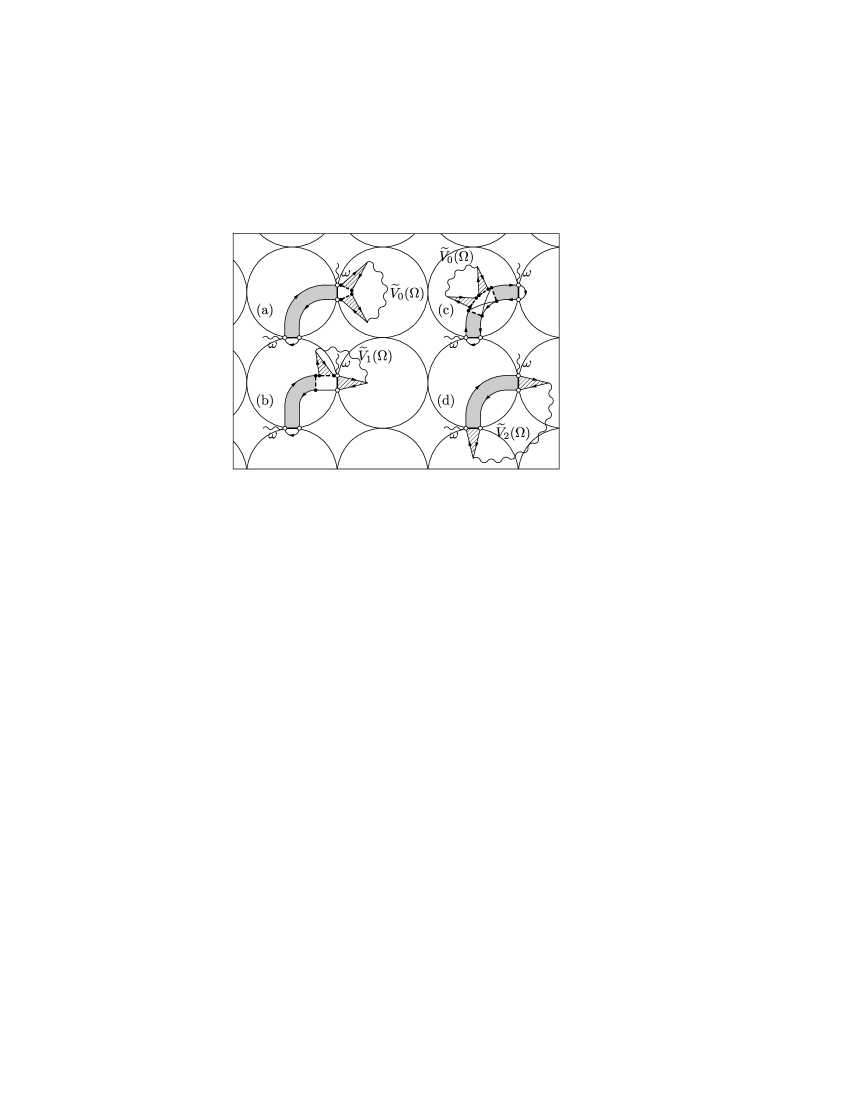
Figure 14: Diagrams for the interaction corrections to Hall conductivity arising from spatial scales of the order of the grain size (“short-scale” contributions) at arbitrary compared to $\Gamma$ temperatures $T$. Gray blocks denote nonzero-mode intragrain diffusons $\bar{D}(0,{\bf r},{\bf r}^{\prime})$ [Eq. (42)], whereas rendered with lines blocks denote zero-mode diffusons $\mathcal{D}_{0}(\Omega,{\bf i},{\bf j})$ [Eq. (51)] of the whole system.

One possibility is to leave the “central” diffuson as it is in Fig. 12, i.e., as a non-zero-mode diffuson $\bar{D}(\omega,{\bf r},{\bf r}^{\prime})$ of a single grain, and to take “adjacent” diffusons as zero-mode diffusons $\mathcal{D}_{0}(\Omega,{\bf i},{\bf j})$ [Fig. 14(d)]. This gives the contribution analogous to Eq. (85d):

$$\alpha_{\text{d}}\lambda^{\text{d}}_{n}(\omega,\Omega)=2\widetilde{V}_{2}(\Omega)\frac{1}{\gamma_{n}},$$ (106d)

where $\widetilde{V}_{2}(\Omega)=\widetilde{V}(\Omega,{\bf i}+{\bf e}_{x},{\bf i}+{\bf e}_{y})$. The rest of the diagrams arising from the diagram (d) in Fig. 12 are discussed in the next section.

Let us sum the contributions (106a), (106b), (106c), and (106d). For the corresponding correction

$$\delta\Pi_{xy}(\omega)=\frac{g_{T}^{2}}{\nu}\sum_{n>0}f_{n}T\sum_{\Omega>0}\theta_{\omega,\Omega}\sum_{i=\text{a},\text{b},\text{c},\text{d}}\alpha_{i}\lambda^{(i)}_{n}(\omega,\Omega)$$

to the bare current-current correlation function $\Pi^{(0)}_{xy}(\omega)$ [Eq. (65)] we obtain

$$\delta\Pi_{xy}(\omega) = -2\frac{g_{T}^{2}}{\nu}\sum_{n>0}f_{n}T\sum_{\Omega>0}\theta_{\omega,\Omega}\times$$ (107)

$$\times \frac{1}{\gamma_{n}}[3\widetilde{V}_{0}(\Omega)-2\widetilde{V}_{1}(\Omega)-\widetilde{V}_{2}(\Omega)].$$

Compare the correction (107) with the correction (95) obtained in the regime $T\gg\Gamma$, in which $\Omega,T\ll E_{\text{Th}}$ was also assumed. Equation (107) differs from Eq. (95) only by having $\mathcal{D}_{0}(\Omega,{\bf q})=1/(\Omega+\Gamma_{\bf q})$ instead of $1/\Omega$ for the diffusons renormalizing the interaction vertices. This difference is relevant at $T,\Omega\lesssim\Gamma$, when tunneling comes into play. Nevertheless, the correction (107) still arises from the spatial scales of the order of the grain size $a$, even if $T\ll\Gamma$. At $T,\Omega\gg\Gamma$, when one can neglect tunneling in Eq. (107) [$\mathcal{D}_{0}(\Omega,{\bf q})\rightarrow 1/\Omega$], the corrections (107) and (95) coincide.

To get a temperature dependence of the correction (107) we note that the summed over $\Omega$ expression is still proportional to $1/\Omega$ in the wide range $\Gamma\lesssim\Omega\lesssim g_{T}E_{c}$, giving a logarithmic contribution. The question about the lower cut-off is easily resolved: it equals $T$ at $T\gg\Gamma$ and $\Gamma$ at $T\ll\Gamma$. Thus, the lower cut-off is $\max(T,\Gamma)$. To get a correct upper cut-off we separate Eq. (107) artificially into two parts according to the form of Eqs. (87),(88):

$$\delta\Pi_{xy}(\omega)=\delta\Pi^{TA}_{xy}(\omega)+\delta\Pi^{VD}_{xy}(\omega),$$

where

$$\delta\Pi^{TA}_{xy}(\omega)=-8\frac{g_{T}^{2}}{\nu}\sum_{n>0}f_{n}T\sum_{\Omega>0}\theta_{\omega,\Omega}\frac{1}{\gamma_{n}}\frac{1}{\Omega^{2}}\left[\widetilde{V}_{0}(\Omega)-\widetilde{V}_{1}(\Omega)\right]$$ (108)

and

$$\delta\Pi^{VD}_{xy}(\omega) = 2\frac{g_{T}^{2}}{\nu}\sum_{n>0}f_{n}T\sum_{\Omega>0}\theta_{\omega,\Omega}\,\frac{1}{\gamma_{n}}\times$$ (109)

$$\times \frac{1}{\Omega^{2}}\left[\widetilde{V}_{2}(\Omega)+\widetilde{V}_{0}(\Omega)-2\widetilde{V}_{1}(\Omega)\right].$$

Keeping in mind that Eqs. (108) and (109) must match with Eqs. (87) and (88) at $\Omega\sim E_{\text{Th}}$, we have to attribute a cut-off $g_{T}E_{c}$ to $\delta\Pi^{TA}_{xy}(\omega)$ and $\min(g_{T}E_{c},E_{\text{Th}})$ to $\delta\Pi^{VD}_{xy}(\omega)$. Doing so, for the corresponding corrections to HC we obtain

$$\frac{\delta\sigma^{TA}_{xy}(T)}{\sigma^{(0)}_{xy}}=-\frac{1}{\pi g_{T}d}\ln\left[\frac{g_{T}E_{c}}{\max(T,\Gamma)}\right]\mbox{ for }T\lesssim g_{T}E_{c}$$ (110)

and

$$\frac{\delta\sigma^{VD}_{xy}(T)}{\sigma^{(0)}_{xy}}=\frac{c_{d}}{4\pi g_{T}}\ln\left[\frac{\min(g_{T}E_{c},E_{\text{Th}})}{\max(T,\Gamma)}\right]$$ (111)

for $T\lesssim\min(g_{T}E_{c},E_{\text{Th}})$.

Let us write the total correction $\delta\sigma_{xy}$ to HC

$$\sigma_{xy}=\sigma_{xy}^{(0)}+\delta\sigma_{xy}$$

as

$$\delta\sigma_{xy}=\delta\sigma^{TA}_{xy}+\delta\sigma^{VD}_{xy}+\delta\sigma^{AA}_{xy},$$ (112)

where $\delta\sigma^{TA}_{xy}$ and $\delta\sigma^{VD}_{xy}$ are given by Eqs. (110) and (111) and $\delta\sigma^{AA}_{xy}$ comes from the rest of the diagrams, arising from the diagram (d) in Fig. 12 when we take tunneling into account. We consider the latter “large-scale” contribution now.

VI.2.2 Large-scale contribution

Figure 15: Diagrams for the interaction corrections to Hall conductivity arising from large spatial scales at arbitrary compared to $\Gamma$ temperatures $T$. The diagrams (d1) and (d2) cancel each other leading to the vanishing “Altshuler-Aronov” correction to the Hall conductivity: $\delta\sigma_{xy}^{AA}=0$.

As explained above, in order to generalize the diagram (d) in Fig. 12 to include the temperatures $T\lesssim\Gamma$ one has to replace all three diffusons in it by the zero-mode diffusons $\mathcal{D}_{0}$, and then insert a non-zero-mode part $\bar{D}$ [Eq. (42)] of the diffuson $D$ [Eq. (40)] into one of the grains. Having considered the diagram (d) in Fig. 14, we are left with two following possibilities.

(i) One can insert the non-zero-mode part $\bar{D}$ [Eq. (42)] somewhere into the middle of one of the three diffusons $\mathcal{D}_{0}$. One can show straightforwardly that all the contributions from such diagrams, when summed up, cancel each other exactly.

(ii) The less trivial possibility is to consider nonzero modes $\bar{D}$ in the grains directly adjacent to the contacts $({\bf i}+{\bf e}_{x},{\bf i})$ and $({\bf j}+{\bf e}_{y},{\bf j})$, corresponding to external current vertices for the correlation function $\Pi_{xy}(\omega,{\bf i},{\bf j})$, i.e., in the grains ${\bf i}+{\bf e}_{x}$ or ${\bf i}$ for contact $({\bf i}+{\bf e}_{x},{\bf i})$ and in the grains ${\bf j}+{\bf e}_{y}$ or ${\bf j}$ for contact $({\bf j}+{\bf e}_{y},{\bf j})$. However, the total contribution from such diagrams also vanishes: for each diagram of this type there exists another diagram, the contribution of which is exactly opposite and, consequently, their sum is zero. One of such pairs are the diagrams (d1) and (d2) shown Fig. 15, their contributions to the current-current correlation function being

$$\delta\Pi^{\text{d1}}_{xy}(\omega) = \frac{g_{T}^{2}}{\nu}2T\sum_{\Omega>0}\theta_{\omega,\Omega}D_{>}\times$$

$$\times \sum_{\bf j}\Gamma\mathcal{D}_{0}(\omega+\Omega,{\bf i},{\bf j}+{\bf e}_{x})\widetilde{V}(\Omega,{\bf j}-{\bf e}_{y},{\bf i}+{\bf e}_{x}),$$

$$\delta\Pi^{\text{d2}}_{xy}(\omega) = -\frac{g_{T}^{2}}{\nu}2T\sum_{\Omega>0}\theta_{\omega,\Omega}D_{>}\times$$

$$\times \sum_{\bf j}\Gamma\mathcal{D}_{0}(\omega+\Omega,{\bf i},{\bf j}-{\bf e}_{y})\widetilde{V}(\Omega,{\bf j}-{\bf e}_{x},{\bf i}+{\bf e}_{x}).$$

Here $D_{>}$ is the non-zero-mode intragrain diffuson connecting contacts in the counterclockwise direction, i.e., in the direction of the edge drift. Using the translational invariance and symmetry in each component of the zero-mode diffuson $\mathcal{D}_{0}$ and the screened Coulomb interaction $\widetilde{V}$, e.g., that $\mathcal{D}_{0}(\Omega,{\bf i}-{\bf j})=\mathcal{D}_{0}(\Omega,i_{x}-j_{x},i_{y}-j_{y})=\mathcal{D}_{0}(\Omega,j_{x}-i_{x},i_{y}-j_{y})$, we obtain that the sum over ${\bf j}$ in $\delta\Pi^{\text{d2}}_{xy}(\omega)$ is identical to the one in $\delta\Pi^{\text{d1}}_{xy}(\omega)$, and thus the contributions cancel each other:

$$\delta\Pi^{\text{d1}}_{xy}(\omega)+\delta\Pi^{\text{d2}}_{xy}(\omega)=0.$$

Therefore, we obtain that the total contribution from the diagrams of types (i) and (ii) vanishes identically:

$$\delta\sigma_{xy}^{AA}=0.$$ (113)

As a result, all nonvanishing contributions to HC at arbitrary compared to $\Gamma$ temperatures $T$ are given by the diagrams (a),(b),(c),(d) in Fig. 14, which lead to the corrections (110) and (111). Note that these contributions arise from the spatial scales of the order of the grain size $a$, even for temperatures $T\ll\Gamma$. On the contrary, the eventually vanishing contributions of the diagrams of types (i) and (ii) [as (d1) and (d2) in Fig. 15] arise from the spatial scales exceeding $a$. The reason is that in these diagrams the contacts with external tunneling vertices are connected by the diffuson $\mathcal{D}_{0}(\Omega,{\bf q})$, which “size” in the real space is determined by the thermal length $L_{T}^{*}=\sqrt{\Gamma a^{2}/T}$. In case of low temperatures $T\ll\Gamma$, the thermal length $L_{T}^{*}\gg a$ can exceed the grain size $a$ significantly.

It is always instructive to compare the results for a granular metal with those for an ordinary homogeneously disordered metal (HDM). For quantities arising from large spatial scales (i.e., much greater than the grain size $a$ for granular metals and the mean free path for diffusive HDMs) one expects correspondence between the two, since at such scales the microscopic structure of the system becomes irrelevant. The first-order Coulomb interaction correction $\delta\sigma_{xy}$ to Hall conductivity of HDM was first studied in Ref. AKLL, and the correction was found to vanish, $\delta\sigma_{xy}=0$. So, indeed, our result (113) for the “large-scale” contribution $\delta\sigma_{xy}^{AA}$ agrees with that for HDMs.

Note that even our approach of calculating $\delta\sigma_{xy}^{AA}$ is quite similar to that of Ref. AKLL, . The authors of Ref. AKLL, calculated $\delta\sigma_{xy}$ perturbatively in magnetic field $H$ (assuming $\omega_{H}\tau_{0}\ll 1$) by inserting “magnetic vertex” $-\frac{e}{mc}{\bf A}\hat{{\bf p}}$ in all possible ways into the diagrams for zero magnetic field. (i) Insertions of magnetic vertex into the diffusons were found to cancel and (ii) insertions of magnetic vertex into the block of Green functions at the current vertices (Fig. 6 in Ref. AKLL, ) were found to cancel. These two steps resemble those (i) and (ii) of our approach, insertion of magnetic vertex corresponding to insertion of non-zero-mode intragrain diffuson $\bar{D}$, which contains all information about magnetic field, into the zero-mode “large-scale” diffusons $\mathcal{D}_{0}$.

We want to stress that the “large-scale” AA contribution $\delta\sigma_{xy}^{AA}$ is not any different physically from the “short-scale” VD contribution $\delta\sigma_{xy}^{VD}$. They both correspond to the process, when electron gets diffusively from the contact $({\bf j}+{\bf e}_{y},{\bf j})$ to the contact $({\bf i}+{\bf e}_{x},{\bf i})$. It just happens, that the contribution $\delta\sigma_{xy}^{VD}$ from the diffusion processes through a single grain does contribute to HC, whereas the total contribution $\delta\sigma_{xy}^{AA}$ to HC from the diffusion through more than one grain vanishes.

As a result of Secs. VI.2.1 and VI.2.2, we obtain that the total correction $\delta\sigma_{xy}$ [Eq. (112)] to HC at arbitrary temperatures $T$ is given by two short-scale contributions $\delta\sigma^{TA}_{xy}$ [Eq. (110)] and $\delta\sigma^{VD}_{xy}$ [Eq. (111)], whereas the large-scale contribution $\delta\sigma^{AA}_{xy}=0$ [(Eq. (113)] vanishes in agreement with the theory of HDMs. For the discussion of the corresponding corrections

$$\delta\rho_{xy}=\delta\rho^{TA}_{xy}+\delta\rho^{VD}_{xy}+\delta\rho^{AA}_{xy}$$

to the Hall resistivity

$$\rho_{xy}=\frac{\sigma_{xy}}{\sigma_{xx}^{2}}=\rho_{xy}^{(0)}+\delta\rho_{xy}.$$

we refer the reader to the Results section II starting from Eq. (12).

VII Conclusion

In conclusion, we presented a theory of the Hall effect in granular metals. In spite of its importance this question has not been addressed before. It turned out that considering only zero intragrain spatial harmonics that was very successful in describing the longitudinal conductivity ET ; BELVreview is not sufficient for calculating Hall conductivity and we were forced to take nonzero harmonics into account. Proceeding in this way we have shown that at high enough temperatures the Hall resistivity is given by the classical expression, from which one can extract the effective carrier density of the system. At lower temperatures, quantum effects come into play, their most significant effect being logarithmic temperature-dependent contributions to the Hall conductivity and resistivity due to Coulomb interaction, which are absent in ordinary disordered metals.

We emphasize, however, that Eqs. (9),(10) give the first-order interaction corrections and the result is valid as long as these correction are small. One could try to account for higher orders using a renormalization group analysis (since the contributions are logarithmic), for example, like the one used for the longitudinal conductivity in Ref. ET, . In order to write down proper renormalization group equations, methods more sophisticated than the present diagrammatic approach are needed.

Concerning the experimental situation related to the theory developed here, the logarithmic dependence $\rho_{xx}(T)=R_{1}-R_{2}\ln T$ of the longitudinal resistivity in good conducting ($g_{T}\gtrsim 1$) granular materials, corresponding to the logarithmic renormalizationET ; BELV of the integrain tunneling conductance $g_{T}$ [Eq. (97)], has been observed experimentally (see Refs. expRxx, ). Clearly, measurements of the Hall resistivity $\rho_{xy}$ of such granular samples could be also performed and our theory could be thus tested. Unfortunately, the known to us experimental papers (Refs. expRxy2, ) on convetional Hall effect in granular materials mostly deal with the systems in the regime of low tunneling conductance $g_{T}\ll 1$, opposite to the metallic regime $g_{T}\gg 1$ studied by us, which does not allow us to make a detailed comparison now. We mention that our theory may be also applied to indium tin oxide (ITO) materials (see, e.g., Refs. ITO ). Another related effect is the anomalous Hall effect in ferromagnetic granular materials Mitra .

We hope that more experiments on this subject will be done in the nearest future and that Hall measurements will evolve into an important method of characterization of granular materials.

We thank Igor S. Beloborodov, Yuli V. Nazarov and Anatoly F. Volkov for illuminating discussions. Part of this work was done at the MPI-PKS Dresden in the framework of the workshop ”Dynamics and Relaxation in Complex Quantum and Classical Systems and Nanostructures”. The work was financially supported by Degussa AG (Germany), SFB Transregio 12, the state of North-Rhine Westfalia, and the European Union.

Appendix A Boundary condition

Figure 16: Diagrams for the current-(radius vector) correlator $\langle j_{\alpha}r_{\beta}\rangle$ [Eq. (119)], if one directly expands Green functions to the linear order in vector potential ${\bf A}$. Fermionic lines denote the Green function $[G(\varepsilon,{\bf p})]^{-1}=i\varepsilon-\xi({\bf p})+\frac{i}{2\tau_{0}}\text{sgn}\,\varepsilon$ of a bulk metal with $H=0$. (a) Magnetic-field-independent part of $\langle j_{\alpha}r_{\beta}\rangle$ giving the LHS of the boundary condition (39). (b) Linear in magnetic field part of $\langle j_{\alpha}r_{\beta}\rangle$ obtained by inserting “magnetic vertex” $-\frac{e}{mc}{\bf A}\hat{{\bf p}}$ in all possible ways into the diagram (a) and giving the RHS of Eq. (39).

To obtain the boundary condition for the diffuson $D(\omega,{\bf r},{\bf r}^{\prime})$ [Eq. (34)], we recall its physical meaning: In the real-time representation, the quantity

$$D(t,{\bf r},{\bf r}^{\prime})=\int_{-\infty}^{+\infty}d\tilde{\omega}e^{-i\tilde{\omega}t}[D(\omega_{n},{\bf r},{\bf r}^{\prime})]|_{\begin{subarray}{c}i\omega_{n}\rightarrow\tilde{\omega}+i0,\\ \omega_{n}>0\end{subarray}}$$

gives the probability density to find an electron at point ${\bf r}$ at time $t$ provided it was at point ${\bf r}^{\prime}$ at time $t=0$. Therefore, according to the formal definition (34) of the diffuson, we can write down the probability current corresponding to the diffusion process as

$${\bf j}(\omega,{\bf r},{\bf r}^{\prime})=\frac{1}{2\pi\nu}\langle\hat{{\bf j}}_{\bf r}\left[\mathcal{G}(\varepsilon+\omega,{\bf r},{\bf r}^{\prime})\mathcal{G}(\varepsilon,{\bf r}^{\prime},{\bf r})\right]\rangle_{U},(\varepsilon+\omega)\varepsilon<0,$$ (114)

where

$$\hat{{\bf j}}_{\bf r}[\mathcal{G}(\varepsilon+\omega,{\bf r},{\bf r}^{\prime})\mathcal{G}(\varepsilon,{\bf r}^{\prime},{\bf r})] = \frac{1}{2m}[\mathcal{G}(\varepsilon,{\bf r}^{\prime},{\bf r})(-i\nabla_{\bf r})\mathcal{G}(\varepsilon+\omega,{\bf r},{\bf r}^{\prime})+$$ (115)

$$+ \mathcal{G}(\varepsilon+\omega,{\bf r},{\bf r}^{\prime})(i\nabla_{\bf r})\mathcal{G}(\varepsilon,{\bf r}^{\prime},{\bf r})]-\frac{e}{mc}{\bf A}({\bf r})\mathcal{G}(\varepsilon+\omega,{\bf r},{\bf r}^{\prime})\mathcal{G}(\varepsilon,{\bf r}^{\prime},{\bf r})$$

is the current operator acting on the product of two Green functions and ${\bf A}({\bf r})$ is a vector potential corresponding to magnetic field ${\bf H}$. Since electron cannot escape from an isolated grain, the normal component of the current ${\bf j}={\bf j}(\omega,{\bf r},{\bf r}^{\prime})$ must vanish at the grain boundary:

$$({\bf n},{\bf j})|_{{\bf r}\in S}=0.$$ (116)

Here, ${\bf n}$ is a unit vector normal to the grain boundary and pointing outside the grain. Equation (116) together with Eqs. (114) and (115) gives a general form of the boundary condition for the diffusion propagator $D(\omega,{\bf r},{\bf r}^{\prime})$. Further simplifications depend on the model used. In the case of white-noise disorder, using the integral equation (37) for the diffuson, we obtain

$${\bf j}(\omega,{\bf r},{\bf r}^{\prime}) = \hat{{\bf j}}_{\bf r}[D_{0}(\omega,{\bf r},{\bf r}^{\prime})]$$ (117)

$$+ \frac{1}{\tau_{0}}\int d{\bf x}\,\hat{{\bf j}}_{\bf r}[D_{0}(\omega,{\bf r},{\bf x})]D(\omega,{\bf x},{\bf r}^{\prime})$$

where $\hat{{\bf j}}_{\bf r}$ acts on the Green functions of $D_{0}(\omega,{\bf r},{\bf r}^{\prime})=G(\varepsilon+\omega,{\bf r},{\bf r}^{\prime})G(\varepsilon,{\bf r}^{\prime},{\bf r})$ as in Eq. (115).

We now exploit the diffusive limit. Since $D_{0}(\omega,{\bf r},{\bf r}^{\prime})$ varies on the spatial scale $l\ll a$, we can (i) neglect the first term in the RHS of Eq. (117); (ii) expand $D(\omega,{\bf x},{\bf r}^{\prime})$ writing it as

$$D(\omega,{\bf x},{\bf r}^{\prime})\approx D(\omega,{\bf r},{\bf r}^{\prime})+({\bf x}-{\bf r})_{\beta}\nabla_{{\bf r}\beta}D(\omega,{\bf r},{\bf r}^{\prime})$$

to get

$$j_{\alpha}(\omega,{\bf r},{\bf r}^{\prime})=\frac{1}{\tau_{0}}\langle j_{\alpha}r_{\beta}\rangle\nabla_{{\bf r}\beta}D(\omega,{\bf r},{\bf r}^{\prime}),$$ (118)

where

$$\langle j_{\alpha}r_{\beta}\rangle=\int d{\bf x}\hat{j}_{{\bf r}\alpha}[D_{0}(\omega,{\bf r},{\bf x})]({\bf x}-{\bf r})_{\beta}$$ (119)

is the current-(radius vector) correlation function. (iii) In the diffusive limit, details of the boundary scattering become unimportant as soon as we move away from the boundary into the bulk of the grain over the distance of the order of the mean free path $l$. Since $D(\omega,{\bf r},{\bf r}^{\prime})$ in Eq. (118) varies on the scales $a\gg l$, the condition (116) may be evaluated not exactly at the boundary, but at some point a few $l$ away from it. This allows us to use for Green functions $G$ in Eq. (119) their expressions for the bulk.

The correlation function $\langle j_{\alpha}r_{\beta}\rangle$ can be calculated via diagrammatic technique either by directly expanding Green functions in vector potential ${\bf A}({\bf r})$ (Fig. 16) or using an explicitly gauge-invariant approach developed by Khodas and Finkel’stein in Ref. Khodas, . Proceeding in either way, in the linear order in $H$ we get

$$\langle j_{\alpha}r_{\beta}\rangle=C\left(\delta_{\alpha\beta}+\frac{e\tau_{0}}{mc}\epsilon_{\alpha\beta\gamma}H_{\gamma}\right),$$ (120)

where $\epsilon_{\alpha\beta\gamma}$ is the totally antisymmetric tensor, $\epsilon_{xyz}=1$, and $C=-(2\pi/3)\nu l^{2}$ is an irrelevant for the boundary condition (116) prefactor. Inserting Eqs. (118) and (120) into Eq. (116), we obtain the boundary condition for the diffuson $D=D(\omega,{\bf r},{\bf r}^{\prime})$ in the presence of magnetic field:

$$n_{\alpha}\left(\delta_{\alpha\beta}+\frac{e\tau_{0}}{mc}\epsilon_{\alpha\beta\gamma}H_{\gamma}\right)\nabla_{{\bf r}\beta}D|_{{\bf r}\in S}=0,$$

which can be easily expressed in the form of Eq. (39).

References

(1) B.L. Altshuler and A.G. Aronov, in Electron-Electron
Interactions in Disordered Systems, edited by A.L. Efros and M. Pollak
(Elsevier, Amsterdam, 1985).
(2) P.A. Lee and T.V. Ramakrishnan, Rev. Mod. Phys. 57, 287
(1985).
(12) I.S. Beloborodov, A.V. Lopatin, and V.M. Vinokur, Phys. Rev.
B 70, 205120 (2004).
(13) Ya.M. Blanter, V.M. Vinokur, and L.I. Glazman Phys. Rev. B
73, 165322 (2006).
(14) C. Biagini, T. Caneva, V. Tognetti, and A.A. Varlamov, Phys.
Rev. B 72, 041102(R) (2005).
(15) M.Yu. Kharitonov, K.B. Efetov, in preparation.
(16) H. Fukuyama, J. Phys. Soc. Japan 49, 644 (1980).
(17) M. Khodas, A. M. Finkel’stein, Phys. Rev. B 68,
155114 (2003).
(18) A.A. Abrikosov, L.P. Gorkov, and I.E. Dzyaloshinski,
Methods of Quantum Field Theory in Statistical Physics (Prentice-Hall,
Englewood Cliffs, New Jersey, 1963).
(20) L.D. Landau and E.M. Lifshitz, Electrodynamics of
Continuous Media, Course of Theoretical Physics, Vol. 8 (Pergamon, New
York, 1975).
(21) A.M. Finkelstein, Sov. Phys. JETP 57, 97 (1983); C.
Castellani, C. Di Castro, P.A. Lee, and M. Ma, Phys. Rev. B 30, 527
(1984).
(22) G. Zala, B.N. Narozhny, and I.L. Aleiner, Phys. Rev. B 64, 214204 (2001).
(23) L.P. Gorkov, A.I. Larkin, and D.E. Khmelnitskii, Sov. Phys.
JETP Lett. 30, 228 (1979); S. Hikami, Phys. Rev. B 24,
2671 (1981).
(24) M.V. Feigel’man, A.S. Ioselevich, M.A. Skvortsov, Phys. Rev.
Lett. 93, 136403 (2004).
(25) B.L. Altshuler and A.G. Aronov, Solid State Commun.
30, 115 (1979).
(26) B.L. Altshuler and A.G. Aronov, Solid State Commun.
46, 429 (1983).
(27)
R.W. Simon, B.J. Dalrymple, D.V. Vechten, W.W. Fuller, and S.A. Wolf, Phys. Rev. B
36, 1962 (1987);
H. Fujimori, S. Mitani, S. Ohnuma, T. Ikeda, T. Shima, and T. Masumoto, Mater. Sci. Eng.,
A 181, 897 (1994);
A. Gerber, A. Milner, G. Deutscher, M. Karpovsky, and A.
Gladkikh, Phys. Rev. Lett. 78, 4277 (1997);
L. Rotkina, S. Oh, J. N. Eckstein, and S. V. Rotkin
Phys. Rev. B 72, 233407 (2005).
(28) X.X. Zhang, Chuncheng Wan, H. Liu, Z.Q. Li, Ping Sheng, J.J. Lin, Phys. Rev. Lett.
86, 5562 (2001);
B. Bandyopadhyay, P. Lindenfeld, W.L. McLean, and H.K. Sin Phys. Rev. B 26, 3476
(1982);
M. Nissim and R.L. Rosenbaum Phys. Rev. B 40, 10629 (1989);
T.T.M. Palstra, R.C. Haddon, A.F. Hebard, and J. Zaanen Phys. Rev. Lett. 68, 1054
(1992);
X.N. Jing, N. Wang, A.B. Pakhomov, K.K. Fung, and X. Yan Phys. Rev. B 53,
14032 (1996).
(29) J. Ederth et al, Phys. Rev. B 68, 155410
(2003); J. Ederth et al, Thin Solid Films. 445, 199 (2003).
(30) P. Mitra, A. F. Hebard, K.A. Muttalib, P. Woelfle,
cond-mat/0606215.