The local star formation history of the thin disc derived from kinematic data

Abstract

Context. We present an evolutionary disc model for the thin disc in the solar cylinder based on a continuous star formation history (SFR) and a continuous dynamical heating (AVR) of the stellar subpopulations.

Aims. We determine the star formation history of the thin disc in the solar vicinity. The self-consistent model of the vertical structure allows predictions of the density, age, metallicity and velocity distribution of main sequence stars as a function of height above the midplane.

Methods. The vertical distribution of the stellar subpopulations are calculated self-consistently in dynamical equilibrium. The SFR and AVR of the stellar subpopulations are determined by fitting the velocity distribution functions of main sequence stars.

Results. We find a vertical disc model for the thin disc including the gas and dark matter component, which is consistent with the local kinematics of main sequence stars and fulfils the known constraints on the surface densities and mass ratios. The SFR shows a maximum 10 Gyr ago declining by a factor of 10 until present time. The velocity dispersion of the stellar subpopulations increase with age according to a power law with index 0.375. Using the new scale heights leads to a best fit IMF with power-law indices of 1.5 below and 4.0 above 1.6$\rm{M}_{\mathrm{\rm\sun}}$, which has no kink around 1$\rm{M}_{\mathrm{\rm\sun}}$. Including a thick disc component results in slight variations of the thin disc properties, but has a negligible influence on the SFR. A variety of predictions are made concerning the number density, age and metallicity distributions of stellar subpopulations as a function of $z$ above the galactic plane.

Conclusions. The combination of kinematic data from Hipparcos and the finite lifetimes of main sequence stars allows strong constraints on the structure and history of the local disc. A constant SFR can be ruled out.

1 Introduction

The star formation history $SFR(t)$ of the Milky Way disc is still not very well determined. The main reason for that is the lack of good age estimators with corresponding unbiased stellar samples. Especially samples selected by colour cuts or by a magnitude limit are biased with respect to the age distribution, because there is an age-metallicity relation due to the chemical enrichment of the disc. Therefore not even the famous Geneva-Copenhagen sample of 14.000 F and G stars (Nordstroem et al. nor04 (2004)) with well determined stellar properties including individual age estimates can be used to derive the star formation history directly by star counts. The most complete disc model based on star counts is that of Robin et al. (rob03 (2003)). They used a series of stellar subpopulations of different ages including the AVR and the chemical enrichment but fixing the $SFR$ to be constant. As a result, scale heights and surface densities of the stellar subpopulations are systematically smaller than in our model. Rocha-Pinto et al. (roc00 (2000)) used chromospheric age determinations of late type dwarfs. They apply stellar evolution and scale height corrections. The main result is the determination of enhanced star formation episodes over the lifetime of the disc. They exclude a constant $SFR$ from chemical evolution models. In R. & C. de la Fuente Marcos (fue04 (2004)) the star formation history for open star clusters were determined. They found at least five episodes of enhanced star formation in the last 2 Gyr. Since star cluster contain only a small percentage of all disc stars, an extrapolation to the total (smoothed) $SFR$ is not possible.

In recent years the Hipparcos stars with precise parallaxes and proper motions were used to determine the $SFR$ with different methods. Hernandez et al. (her00 (2000)) determined the $SFR$ over the last 3 Gyr using isochrone ages. They found a series of star formation episodes on top of an underlying smooth $SFR$. This result is complementary to our model, which gives the slow evolution of the smoothed $SFR$. In Binney et al. (bin00 (2000)) and in Cignoni et al. (cig06 (2006)) the scale height variation of main sequence stars were not taken into account. Therefore these models derive the local age distribution of K and M dwarfs (with lifetimes larger than the age of the disc) instead of the $SFR$. Binney et al. (bin00 (2000)) determined an age of the thin disc of 11.2 Gyr (consistent with the 12 Gyr we are using) and both papers found an approximately constant age distribution, which is fully consistent with our model.

We present the first disc model, which determines the $SFR$, the $AVR$ and scale heights consistently. We use the Hipparcos stars and at the faint end the Catalogue of Nearby Stars (CNS4) to construct an evolutionary disc model including the kinematic information. We select the main sequence stars and divide these into a series of volume complete subsamples from B to K type. In a kinematic model we derive the vertical velocity distribution functions $f(|W|)$ of each subsample, which depends mainly on the star formation history and the dynamical evolution of the disc described by the dynamical heating $\sigma_{\mathrm{W}}(t)$ (the age velocity dispersion relation AVR). The derived $SFR$ depends on the normalized velocity distribution functions only. Therefore the model is essentially independent of the adopted $IMF$. In a final step we use the disc model to derive the local $IMF$ from the volume complete subsamples applying consistently the lifetime and the scale height corrections.

2 Disc Model

In this section we describe the construction of the disc model and the determination of the properties of the stellar subsamples. For the self-consistent determination of the gravitational potential we take into account the stellar component, the gas component and the dark matter halo.

We use a thin, self-gravitating disc composed of a sequence of stellar subpopulations according to the $SFR$ and the AVR. Additionally a cold gas component and a Dark Matter halo are included for the gravitational forces. We take into account finite lifetimes of the stars and mass loss due to stellar evolution. The stellar remnants stay in their subpopulation, the expelled gas (stellar winds, PNs, and SNs) is mixed implicitly into the gas component. Since the lifetimes and mass loss depend on metallicity, the metal enrichment with time is included. A standard $IMF$ is used for the determination of the stellar mass fraction of the subpopulations with age.

From large sets of template functions for the $SFR$ and AVR we search for the best fitting pair of input functions. The total gravitational potential and the density profile of each age-bin are determined self-consistently assuming isothermal distribution functions with velocity dispersion according to the AVR. The velocity distribution functions $f(|W|)$ for main sequence stars are calculated by a superposition of the Gaussians weighted by the local density contribution up to the lifetime of the stars. These distribution functions are simultaneously compared to the observed $f(|W|)$ in magnitude bins along the main sequence to judge the quality of the model.

2.1 Self-gravitating disc

The backbone of the disc is a self-gravitating vertical disc profile including the gas component in the thin disc approximation. In this approximation the Poisson-Equation is one-dimensional and in the case of a purely self-gravitating thin disc (i.e. no external potential) the Poisson equation can be integrated leading to

$$\left(\frac{\mbox{\rm d}\Phi}{\mbox{\rm d}z}\right)^{2}=8\pi G\int_{0}^{\Phi}\rho(\Phi^{\prime})\mbox{\rm d}\Phi^{\prime}\quad.$$ (1)

Therefore we model all gravitational components by a thin disc approximation. We include in the total potential $\Phi$, the stellar component $\Phi_{\mathrm{s}}$, the gas component $\Phi_{\mathrm{g}}$, and the dark matter halo contribution $\Phi_{\mathrm{h}}$

$$\Phi(z)=\Phi_{\mathrm{s}}(z)+\Phi_{\mathrm{g}}(z)+\Phi_{\mathrm{h}}(z)\quad.$$ (2)

In order to obtain the force of a spherical halo correctly in the thin disc approximation, we use a special approximation (see subsection 2.4). Since we construct the disc in dynamical equilibrium, the density of the sub-components are given as a function of the total potential $\rho_{\mathrm{j}}(\Phi)$. The vertical distribution is given by the implicit function $z(\Phi)$ via direct integration

$$z(\Phi)=\int_{0}^{\Phi}\mbox{\rm d}\Phi^{\prime}\left[8\pi G\int_{0}^{\Phi^{\prime}}\rho(\Phi^{\prime\prime})\mbox{\rm d}\Phi^{\prime\prime}\right]^{-1/2}\quad.$$ (3)

The relative contribution of the stellar, the gaseous, and the DM-component to the surface density (up to $|z|=z_{\mathrm{max}}$) are given by the input parameters $Q_{\mathrm{s}},Q_{\mathrm{g}},Q_{\mathrm{h}}$, which have to be iterated to fit all observational constraints. The disc model has two global scaling parameters to convert the normalized model to physical quantities. We fix the local stellar density to $\rho_{\mathrm{s0}}=0.039\,\rm{M}_{\mathrm{\rm\sun}}\,pc^{-3}$, which is the best observed quantity for the local disc model (Jahreiß et al. jah97 (1997)). The second scaling parameter is the exponential scale height $z_{\mathrm{s}}$, which fixes via the shape correction the half-thickness of the stellar disc $h_{\mathrm{eff}}$, with the mass fractions $Q_{\mathrm{s}},Q_{\mathrm{g}},Q_{\mathrm{h}}$ the surface densities, and via the maximum velocity dispersion $\sigma_{\mathrm{e}}$ the scaling of the velocity distribution functions.

2.2 Stellar disc

The stellar component is composed by a sequence of isothermal subpopulations characterized by the IMF, the chemical enrichment $\mathrm{[Fe/H]}(t)$, the star formation history $SFR(\tau)$, and the dynamical evolution described by the vertical velocity dispersion $\sigma_{\mathrm{W}}(t)$. Here $\tau=t_{\mathrm{a}}-t$ is the time and $t$ is the age of the subpopulation running back in time from the present time $t_{\mathrm{a}}=12$ Gyr (which is the adopted age of the disc). We include mass loss due to stellar evolution and retain the stellar-dynamical mass fraction $g(t)$ (stars + remnants) only. The mass lost by stellar winds, supernovae and planetary nebulae is mixed implicitly to the gas component.

With the Jeans equation the vertical distribution of each isothermal subpopulation is given by

$$\rho_{\mathrm{s,j}}(z)=\rho_{\mathrm{s0,j}}\exp\left(\frac{-\Phi(z)}{\sigma^{2}_{\mathrm{W,j}}}\right)\quad,$$ (4)

where $\rho_{\mathrm{s,j}}$ is actually a ’density rate’, the density per age bin, and $\sigma_{\mathrm{W,j}}$ the velocity dispersion at age $t_{\mathrm{j}}$. The connection to the $SFR$ is given by the integral over $z$

$$g(t_{\mathrm{j}})SFR(\tau_{\mathrm{j}})=\int_{\mathrm{-\infty}}^{\infty}\rho_{\mathrm{s,j}}(z)\mbox{\rm d}z\quad.$$ (5)

with time $\tau_{\mathrm{j}}=t_{\mathrm{a}}-t_{\mathrm{j}}$. The (half-)thickness $h_{\mathrm{p}}(t_{\mathrm{j}})$ of the subpopulations is defined by the midplane density $\rho_{\mathrm{s0,j}}$ through

$$\rho_{\mathrm{s0,j}}=\frac{g(t_{\mathrm{j}})SFR(\tau_{\mathrm{j}})}{2h_{\mathrm{p}}(t_{\mathrm{j}})}\quad.$$ (6)

and can be calculated by

$$h_{\mathrm{p}}(t_{\mathrm{j}})=\int_{0}^{\infty}\frac{\rho_{\mathrm{s,j}}(z)}{\rho_{\mathrm{s0,j}}}\mbox{\rm d}z=\int_{0}^{\infty}\exp\left(\frac{-\Phi(z)}{\sigma^{2}_{\mathrm{W,j}}}\right)\mbox{\rm d}z\quad.$$ (7)

The total stellar density $\rho_{\mathrm{s}}(z)$ and velocity dispersion $\sigma_{\mathrm{s}}(z)$ are determined by

$$\rho_{\mathrm{s}}(z) = \int_{0}^{t_{\mathrm{a}}}\rho_{\mathrm{s,j}}(z)\mbox{\rm d}t$$ (8)

$$\sigma^{2}_{\mathrm{s}}(z) = \frac{1}{\rho_{\mathrm{s}}(z)}\int_{0}^{t_{\mathrm{a}}}\sigma^{2}_{\mathrm{W,j}}\rho_{\mathrm{s,j}}(z)\mbox{\rm d}t\quad.$$ (9)

$\rho_{\mathrm{s}}(z)$ then determines the potential $\Phi_{\mathrm{s}}(z)$ via the Poisson equation. The total stellar surface density $\Sigma_{\mathrm{s}}$ is connected to the integrated star formation $S_{0}$ by the effective stellar-dynamical mass fraction $g_{\mathrm{eff}}$

$$\Sigma_{\mathrm{s}}=\int\rho_{\mathrm{s}}(z)\mbox{\rm d}z=g_{\mathrm{eff}}S_{0}$$ (10)

with

$$S_{0}=\int SFR\,\mbox{\rm d}t\quad\mbox{and}\quad g_{\mathrm{eff}}=\frac{\int g(t)SFR(\tau)\mbox{\rm d}t}{S_{0}}\quad,$$ (11)

which includes luminous stars and stellar remnants. The local stellar density is given by

$$\rho_{\mathrm{s0}}=\frac{g_{\mathrm{eff}}S_{0}}{2h_{\mathrm{eff}}}$$ (12)

with thickness $h_{\mathrm{eff}}$ for all stars. For a general shape of the density profile $h_{\mathrm{eff}}$ is different to $z_{\mathrm{s}}$, the exponential scale height well above the midplane. The effective exponential scale height $z_{\mathrm{s}}$ of the stellar disc describing the exponential decline above the midplane is connected to the maximum velocity dispersion $\sigma_{\mathrm{e}}$ of the subpopulations and the total surface density $\Sigma_{\mathrm{tot}}$ via

$$z_{\mathrm{s}}=C_{\mathrm{z}}z_{\mathrm{e}}=C_{\mathrm{z}}\frac{\sigma_{\mathrm{e}}^{2}}{2\pi G\Sigma_{\mathrm{tot}}}\quad,$$ (13)

where $z_{\mathrm{e}}$ is the exponential scale height of an isothermal component above a disc with total surface density $\Sigma_{\mathrm{tot}}$. The shape correction factor $C_{\mathrm{z}}$ is of order unity and is determined by the mean exponential scale height in the range $z=(2-5)\,z_{\mathrm{e}}$.

The metallicity $\mathrm{[Fe/H]}$ affects the lifetimes, luminosities and colours of the stars and as a consequence also the mass loss of the subpopulations. In order to account for the influence of the metal enrichment we include a metal enrichment $\mathrm{[Fe/H]}(t)$ (see Fig. 1), which leads to a local metallicity distribution of late G dwarfs consistent with the observations (see Fig. 11). The properties of the stars and the stellar subpopulations are determined by population synthesis calculations (see Sect. 2.5).

The properties of main sequence stars with lifetime $\tau$ are determined by an appropriate weighted average over the age range. The thickness $h_{\mathrm{ms}}$, the normalized density profile $\rho_{\mathrm{ms}}(z)/\rho_{\mathrm{ms,0}}$ and the velocity dispersion $\sigma_{\mathrm{ms}}$ are given by

$$h_{\mathrm{ms}}^{-1} = \frac{1}{S_{\tau}}\int_{0}^{\tau}\frac{SFR(\tau)}{h_{\mathrm{p}}(t)}\mbox{\rm d}t$$ (15)

$$\qquad\mathrm{with}\quad S_{\tau}=\int_{0}^{\tau}SFR(\tau)\mbox{\rm d}t$$

$$\frac{\rho_{\mathrm{ms}}(z)}{\rho_{\mathrm{ms,0}}} = \frac{1}{S_{\tau}}\int_{0}^{\tau}h_{\mathrm{ms}}\frac{SFR(\tau)}{h_{\mathrm{p}}(t)}\exp\left(\frac{-\Phi(z)}{\sigma^{2}_{\mathrm{W}}(t)}\right)\mbox{\rm d}t$$ (16)

$$\sigma^{2}_{\mathrm{ms}}(z) = \int_{0}^{\tau}\sigma^{2}_{\mathrm{W}}(t)\frac{SFR(\tau)}{h_{\mathrm{p}}(t)}\exp\left(\frac{-\Phi(z)}{\sigma^{2}_{\mathrm{W}}(t)}\right)\mbox{\rm d}t\times$$ (18)

$$\left[\int_{0}^{\tau}\frac{SFR(\tau)}{h_{\mathrm{p}}(t)}\exp\left(\frac{-\Phi(z)}{\sigma^{2}_{\mathrm{W}}(t)}\right)\mbox{\rm d}t\right]^{-1}\quad.$$

Density profiles and thicknesses of the final model are shown in Figs. 8 and 9 and the velocity dispersion of the main sequence stars are compared in the lower panel of Fig. 5 with the observations.

In the fitting procedure (Sect. 4.1) a pair of star formation history and heating function is selected to derive the intrinsic structure of the disc. The star formation history and heating function of the final model are shown in Fig. 1.

Figure 1: The upper panel shows the $SFR$ for the model and the infall rate of primordial gas derived from a local chemical evolution model (see Sect. 4.5). The thin line is the mean value of the SFR for comparison. The next panel gives the velocity dispersion of the stellar subpopulations The lower panel shows the adopted metal enrichment $\mathrm{[Fe/H]}(t)$, which leads to a local metallicity distribution of late G dwarfs consistent with the observations (see Fig. 11).

2.3 Gas component

For the gas component we use a simple model to account for the gravitational potential of the gas. The vertical profile of the gas component, which is used for the gravitational force of the gas, is constructed dynamically like the stellar component. The gas distribution is modeled by distributing the gas with a constant rate over the velocity dispersion range $\sigma_{\mathrm{W}}(t)$ of the young stars up to a maximum age $t_{\mathrm{g}}$. By varying $t_{\mathrm{g}}$ we force the scale height of the gas $z_{\mathrm{g}}$ to the observed value of $z_{\mathrm{g}}\approx 100$ pc. The surface density of the gas is related to the stellar surface density by the ratio $Q_{\mathrm{g}}/Q_{\mathrm{s}}=\Sigma_{\mathrm{g}}/\Sigma_{\mathrm{s}}$, which is chosen (together with the scale height $h_{\mathrm{eff}}$ of the stars) to be consistent with the observed surface density of $\Sigma_{\mathrm{g}}\approx 10-13\,\rm{M}_{\mathrm{\rm\sun}}pc^{-2}$.

2.4 Dark matter halo

The halo does not fulfil the thin disc approximation. For a spherical halo we get the vertical component of the force to lowest order from

$$\frac{\mbox{\rm d}\Phi_{\mathrm{h}}}{\mbox{\rm d}z}=\frac{GM_{\mathrm{R}}}{R^{2}}\frac{z}{R}\quad,$$ (19)

with $r^{2}=R^{2}+z^{2}$ and the enclosed halo mass $M_{\mathrm{R}}$ inside radius $R$. Comparing this with the one-dimensional Poisson equation from the thin disc approximation (integrated over $z$ near the midplane to lowest order for small $z$)

$$\frac{\mbox{\rm d}\Phi}{\mbox{\rm d}z}\approx 4\pi G\rho_{0}z$$ (20)

we can use for the local halo density

$$\rho_{\mathrm{h0}}=\frac{M_{\mathrm{R}}}{4\pi R^{3}}$$ (21)

to be consistent with the spherical distribution. This value corresponds exactly to the singular isothermal sphere. Therefore we can use the thin disc approximation also for the halo by using the local halo density $\rho_{\mathrm{h0}}$ and the halo velocity dispersion $\sigma_{\mathrm{h}}$ estimated from the rotation curve by adopting an isothermal spherical halo. The effect of a cored halo, anisotropy and flattening, which would lead to small inconsistencies at large $z$, is neglected here. For other halo profiles correction factors would be necessary introducing some inconsistency in the halo profile description and leading to a different local halo density. The latter is be more important, because the effect of the halo potential on the disc is stronger than the adiabatic contraction of the halo in the disc potential.

We use an isothermal halo component with $\sigma_{\mathrm{h}}\approx 100$ km/s. The halo surface density $\Sigma_{\mathrm{h}}$ is determined in the fitting procedure, because it influences not only the total surface density significantly, but also the shapes of the velocity distribution functions $f(|W|)$ of the stars.

2.5 Stellar population synthesis

For the determination of luminosities, main sequence lifetimes and mass loss we are not interpolating directly evolutionary tracks of a set of stellar masses and metallicities. In order to get a complete coverage of stellar masses we use instead the stellar population synthesis code PEGASE (Fioc & Rocca-Volmerange pegase (1997)) to calculate mass loss and luminosities of “pseudo” simple stellar populations (SSPs). This means that the PEGASE code is used to calculate the integrated luminosities and colour indices for a stellar population created in a single star-burst at different time-steps. These SSPs are then used to assemble a stellar population with a given star formation history, in the sense that the star formation history is assembled by a series of star-bursts. In this way we can assemble stellar populations for varying $SFR$ and metal enrichment $\mathrm{[Fe/H]}$. Our SSPs are modeled by a constant star formation rate with a duration of 25 Myr, the time resolution of the disc model. This is done for a set of different metallicities and intermediate values from the chemical enrichment are modeled by linear interpolation.

The application of the PEGASE code is twofold. On one hand mass loss due to stellar winds, planetary nebulae and supernovae determines $g(t)$, the mass fraction remaining in the stellar component as a function of age $t$. This depends on the $IMF$ and the metal enrichment. We adopt a Scalo-like IMF (Scalo sca86 (1986)) given by

$$\mbox{\rm d}N \propto M^{-\alpha}\mbox{\rm d}M$$ (26)

$$\alpha=\left\{\begin{array}[]{lcc}1.25&&0.08\leq M/\rm{M}_{\mathrm{\rm\sun}}<1\\ 2.35&for&1\leq M/\rm{M}_{\mathrm{\rm\sun}}<2\\ 3.0&&2\leq M/\rm{M}_{\mathrm{\rm\sun}}<100\end{array}\right.\quad.$$

and five different metallicities ([Fe/H]= -1.23, -0.68, -0.38, 0.0, 0.32), which are the input parameters into the code. Fig. 2 shows the mass loss for the different metallicities (thin full lines). The thin lines show the contribution from luminous matter and stellar remnants for the set of input metallicities. The sum of both contributions for each metallicity vary by a few percent only and are therefore not shown. The thick full line shows $g(t)$, the fraction of stellar mass in the present day stellar disc as a function of age including the chemical evolution. For the oldest age-bins about 40% of the stellar mass is lost by stellar evolution. The total fraction of stellar mass $g_{\mathrm{eff}}=0.644$ is indicated by the horizontal line.

In the second application we determine the main sequence lifetimes and luminosities for stellar mass bins. Here we use the PEGASE code to compute V-band luminosities of isochrones in small mass bins. These are needed to estimate the mean main sequence lifetime as a function of the V-band luminosity $M_{\mathrm{V}}$ for the calculation of the velocity distribution functions $f(|W|)$ of these stars. We apply the PEGASE code to piecewise constant $IMF$s for mass-bins with $0.1\rm{M}_{\mathrm{\rm\sun}}$ and for a finer grid of metallicities ([Fe/H]= -0.8, -0.68, -0.5, -0.28, 0.0, 0.20, 0.32). In Fig. 3 we show $M_{\mathrm{V}}$ for the different mass bins as a function of age. The lower panel gives the luminosity evolution along the main sequence for the different metallicities (thin lines) and the age dependence of the stars in the disc model for $M=0.8\,\rm{M}_{\mathrm{\rm\sun}}$ demonstrating the significant variation over the whole age range. The upper panels show the age dependent luminosities for all mass bins. These are again not the luminosity evolutions of the stars but the present day properties of the stellar population taking into account the age-metallicity relation. The vertical lines indicate the estimated mean main sequence lifetimes in the corresponding luminosity bins. The criteria to choose these lifetimes for the determination of the velocity distribution functions $f(|W|)$ in the magnitude bins are discussed in Sect. 4.4.

Figure 2: Mass loss due to stellar evolution. The thin lines show the fraction of luminous mass and of remnants (upper and lower curve, respectively) for the set of metallicities used in the PEGASE code. The thick lines shows the total stellar mass fraction (luminous plus remnants) of the model taking into account the age-metallicity relation.

Figure 3: The lower panel shows the age dependence of the absolute luminosity $M_{\mathrm{V}}$ for stars with $M=0.8\,\rm{M}_{\mathrm{\rm\sun}}$ (averaged over $0.1\,\rm{M}_{\mathrm{\rm\sun}}$). Thin lines are the evolution for different metallicities $\mathrm{[Fe/H]}=-0.8;-0.68;-0.5;-0.28;0.0;0.20;0.32$ and the thick lines shows the present day luminosity of the stars as a function of age taking into account the age-metallicity relation.

3 Observational Data

Each stellar subpopulation, which is on average older than $10^{8}$ yr, is in dynamical equilibrium with respect to the vertical distribution. Therefore they can be used as independent samples to determine the total vertical gravitational potential $\phi(z)$. The velocity distribution functions $f(|W|)$ of the samples depend on the age distribution of the stars. Therefore we use main sequence stars, where $f(|W|)$ is a function of the lifetime of the stars. In order to determine the vertical velocity distribution function $f(|W|)$ in the solar neighbourhood we need kinematically unbiased samples with space velocities.

For the determination of the age velocity dispersion relation we use the McCormick K and M dwarfs (Vyssotsky vys63 (1963)). Detected by a spectroscopic survey they are free from kinematic bias. Altogether 516 stars show reliable distances - almost all from the Hipparcos Catalogue - and space velocity components. For a subsample of about 300 stars Wilson and Woolley (wil70 (1970)) estimated the CaII emission intensity at the H and K lines in a relative scale allowing to construct six different age bins under the assumption of a constant star formation rate ( see Jahreiß and Wielen, 1997). For each bin the vertical velocity dispersion is determined. The mean ages of the bins are rescaled from 10 Gyr to 12 Gyr for the total disc age (see Fig. 5). All these stars are also used to determine the velocity distribution function $f(|W|)$ of stars with lifetime larger than 12 Gyr (see Fig. 6). The number of stars in each individual age bin is too low to obtain reliable $f(|W|)$.

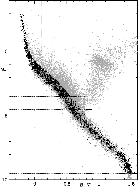
Figure 4: The HR-diagram shows all Hipparcos stars (grey dots) with $\sigma_{\pi}/\pi\leq.10$ The selected main sequence stars are overplotted by larger black dots and the eight magnitude bins are indicated by the dotted lines.

Figure 5: Upper panel: Velocity dispersion as a function of age for the stellar subpopulations. Full symbols are the age groups of the McCormick K and M dwarfs. The asterisks reproduce the age bins of Fig. 31 in Nordström et al. (nor04 (2004)). The full line shows the heating function AVR of the final model. Lower panel: The symbols show the velocity dispersion of the stars along the main sequence (magnitude bins) as a function of mean lifetime. The full line gives the result of the final model.

Figure 6: The normalized velocity distribution functions $f(|W|)$ for the different sub-samples given in Table 1 and for the McCormick stars (lower right). Symbols are the data and lines represent the model.

For the determination of $f(|W|)$ along the main sequence we use the Hipparcos stars with good space velocities supplemented at the faint end down to $M_{\mathrm{V}}=9.5$ mag by stars from an updated version of the Catalogue of Nearby stars (CNS4, Jahreiß et al. jah97 (1997)), i.e. also most of the CNS4 data rely on Hipparcos results. For the determination of the space velocities good distances, proper motions and radial velocities are required. This was achieved in combining the Hipparcos data with radial velocities originating from an unpublished compilation of the ”best” radial velocities for the nearby stars, which was then extended to all Hipparcos stars.

The selection process is a following. The visual absolute magnitude of the Hipparcos stars was determined from the visual magnitude and the trigonometric parallax given in the Hipparcos catalog. In the case of binaries resolved by Hipparcos the $M_{V}$ of the brighter component was chosen calculated from the combined magnitude and the magnitude difference measured by Hipparcos. Then we select in the HR-diagram (Fig. 4) a rough regime along the main sequence in order to exclude most of the giants and white dwarfs. After determination of the best fit for the mean main sequence $M_{\mathrm{V,ms}}(B-V)$ (thick full line) all stars in the magnitude range $M_{\mathrm{V,ms}}\pm 0.8$ mag were selected. Only for the brightest magnitude bin with $M_{\mathrm{V}}<0.5$ mag we use a colour cut $B-V\leq 0.1$ mag instead. Now the main sequence is divided into magnitude bins $M_{\mathrm{V}}<0.5,1\pm 0.5,...,6\pm 0.5,8\pm 1.5$ mag.

In order to avoid a kinematic bias we restrict the distances of the stars in each magnitude bin to be well within the completeness limit of the Hipparcos catalogue determined by the magnitude limit $V\sim 7.3$ mag of the Hipparcos Survey. The properties of the resulting samples of main sequence stars are collected in Table 1. Column 1 lists the source catalogue. Column 2, 3 and 4 list the range in absolute visual magnitude, the selected distance limit, and the total number of stars available, respectively. Column 5 and 6 list the number of stars removed due to poor parallaxes ($\sigma_{\pi}/\pi>.15$) and unknown or poor radial velocities. Finally, in column 7 the remaining number of main sequence stars with good space velocity components is given.

Table 1: Complete samples of nearby main sequence stars

source	$M_{V}$	$d_{lim}$	N	n∗	no RV	Nfin
		[pc]
Hip	$\leq$-0.5	200	93	7	0	86
Hip	0	200	183	27	15	141
Hip	1	100	242	0	1	241
Hip	2	75	401	8	7	386
Hip	3	50	352	0	4	348
Hip	4	30	172	2	0	170
Hip	5	25	172	0	0	172
Hip	6	25	170	0	2	168
CNS	$\geq$6.5	25	525		84	441

(*) n = number of stars with $\sigma_{\pi}/\pi>.15$

For the determination of the velocity distribution functions $f(|W|)$ we correct for the peculiar motion of the Sun using $W_{\odot}=7$ km/s. The resulting normalized distribution functions are shown in Fig. 6 with a binning of 5 km/s in $|W|$.

4 Properties of the disc

The disc model has some free parameters additionally to the main input functions $SFR$ and AVR. In all models we fix the local stellar density to $\rho_{\mathrm{s0}}=0.039\rm{M}_{\mathrm{\rm\sun}}pc^{-3}$ from the CNS4 and the velocity dispersion of the Dark matter halo to $\sigma_{\mathrm{h}}=4\sigma_{\mathrm{e}}$. For each pair of $SFR$ and AVR we determine iteratively the exponential scale height of the stellar disc $z_{\mathrm{s}}$, the relative fractions $Q_{\mathrm{s}},Q_{\mathrm{g}},Q_{\mathrm{h}}$ of the surface density (at $|z|<z_{\mathrm{max}}$, where $z_{\mathrm{max}}$ is indirectly determined by the depth of the potential well), and the scale height of the gas component by choosing a maximum ’age’ $t_{\mathrm{g}}$. The $Q$-values together with $z_{\mathrm{s}}$ determine the maximum velocity dispersion $\sigma_{\mathrm{e}}$ of the stars and the surface densities of the components. A comparison with the observational constraints for the surface densities and velocity dispersions restrict the exponetial scale hwight to $z_{\mathrm{s}}$=270 pc with an uncertainty of 10%. In the final iteration the metal enrichment $\mathrm{[Fe/H]}(t)$ is adapted to be consistent with the local metallicity distribution of G dwarfs. A list of model parameters and derived physical quantities is given in Table 2 together with the corresponding data of other authors.

Table 2: Disc properties: mean and present day $SFR$ (in $\rm{M}_{\mathrm{\rm\sun}}/pc^{2}Gyr$) are for the thin disc; local densities for stellar thin disc, gas, DM halo, thick disc (indices s, g, h, t; in $\rm{M}_{\mathrm{\rm\sun}}/pc^{3}$); surface densities are below $|z_{\mathrm{max}}|=2.3$ kpc or up to 0.35, 1.1 kpc (in $\rm{M}_{\mathrm{\rm\sun}}/pc^{2}$); (half-)thickness of the thin disc $h_{\mathrm{eff}}$ and exponential scale heights $z$ are in pc; velocity dispersions in km/s; The second column represents the thin disc model and the third column the values with the thick disc 1 included. Columns 4 and 5 give some parameters from the literature.

quantity	thin	+ thick	other	sources
	disc	disc
$\langle SFR\rangle$	4.2	3.9
$SFR_{\mathrm{p}}$	0.84	0.79
$\rho_{\mathrm{0}}$	0.094	0.092	0.0761	0.0982
$\rho_{\mathrm{s0}}$	0.039	0.036	0.0451	0.0442
$\rho_{\mathrm{g0}}$	0.042	0.041	0.0211	0.0502
$\rho_{\mathrm{h0}}$	0.013	0.012	0.011
$\rho_{\mathrm{t0}}$		0.003
$\Sigma_{\mathrm{s}}$	32.6	30.3	34.42
$\Sigma_{\mathrm{g}}$	13.4	13.3	61	132
$\Sigma_{\mathrm{t}}$		5.7
$\Sigma_{\mathrm{disc}}$	46.0	49.3	563	484
$\Sigma(<0.35)$	43.2	42.4	413
$\Sigma(<1.1)$	72.0	71.5	743	714
$h_{\mathrm{eff}}$	416	418
$z_{\mathrm{s}}$	270	270
$z_{\mathrm{g}}$	100	101	1401
$z_{\mathrm{t}}$		745
$\sigma_{\mathrm{e}}$	24.4	24.3	17.51
$\sigma_{\mathrm{h}}$	97.5	97.1	851
$\sigma_{\mathrm{t}}$		41.3

¹ Robin et al. rob03 (2003); ² Holmberg & Flynn hol00 (2000); ³ Holmberg & Flynn hol04 (2004); ⁴ Kuiken & Gilmore kui91 (1991)

In the next subsections we discuss the main input functions $SFR$ and AVR and other properties of the disc model including a comparison with other work and predictions for future observations.

4.1 Star formation history and dynamical heating

For a given stellar density profile there is a series of function pairs ($SFR$,AVR) to construct a dynamical equilibrium model. Strong additional constraints originate in the correlation of the velocity distribution functions $f(|W|)$ of stars with different lifetimes. This leads to restrictions for the AVR and in turn to the $SFR$. The sequence of $f(|W|)$ along the main sequence is a direct measure of the age distribution of stars in the local volume, which are converted to surface densities for connecting to the $SFR$.

In the final model we use the star formation history (see Fig. 1)

$$SFR(\tau) = S_{0}\frac{a(\tau+t_{0})}{(\tau^{2}+b^{2})^{2}}\quad\mathrm{with}$$ (27)

$$a = 34.5\,;\quad b=4.2\,;\quad t_{0}=0.01\,,$$ (28)

where the time $\tau$ is in units of Gyr and $S_{0}=50.5\,\rm{M}_{\mathrm{\rm\sun}}/pc^{2}$ is connected to the stellar surface density by Eq. 10. The $SFR$ decreases by a factor of 10 from the maximum to the present day value, which corresponds to an e-folding timescale of 5 Gyr. The present day star formation rate with 20% of the average value of 4.1 $\rm{M}_{\mathrm{\rm\sun}}/pc^{2}Gyr$ is relatively low. It is confirmed by the $IMF$ considerations (see Sect. 4.7).

For the dynamical heating function AVR (see Fig. 5) we use a power law

$$\sigma_{\mathrm{W}}(t) = \sigma_{\mathrm{e}}\left(\frac{t+t_{0}}{t_{\mathrm{a}}+t_{0}}\right)^{\alpha}\quad\mathrm{with}$$ (29)

$$\alpha = 0.375\,;\quad t_{0}=0.0767\,,$$ (30)

where $t$ is the age in Gyr. The velocity dispersion of newly born stars is $\sigma_{\mathrm{p}}=0.15\sigma_{\mathrm{e}}$ and $\sigma_{\mathrm{e}}=24.4$ km/s is the maximum velocity dispersion of the oldest stars with an age of $t_{\mathrm{a}}=12$ Gyr. The power law index $\alpha=0.375$ is in the range of the classical value of 1/2 from Wielen (wie77 (1977)), of 0.47 (Nordström et al. nor04 (2004)) and the value of 1/3 derived by Binney et al. (bin00 (2000)) from proper motion measurements.

4.2 Density profiles

The vertical density profiles of the gas and of the stars are flattened at the galactic plane. A measure of the flattening is given by the ratio of the thickness and the exponential scale height.

The corresponding stellar disc scale height is $z_{\mathrm{s}}=270$ pc (from Eq. 13 with $C_{\mathrm{z}}=1.18$), whereas the half-thickness $h_{\mathrm{eff}}$ is 50% larger.

For the gas, the thickness is 160 pc compared to the scale height of 100 pc. The density profile and the surface density is consistent with the observed HI-profile (Dickey & Lockman (dic90 (1990)) taking into account about 50% of H₂ (Bronfman et al. (bro88 (1988)) within the large uncertainty range.

Due to the gravitational potential of the disc, the local density of the dark matter halo is 55% larger than the DM density at $z=2.3$ kpc and 18% larger than the mean DM density.

Figure 7: Vertical profiles of the disc. From top to bottom: Density profiles of the components; $K_{\mathrm{z}}$ force, which is proportional to the cumulative surface density; velocity dispersion of the stellar component; V-band luminosity weighted mean metallicity of the stellar component.

Figure 8: Upper panel: Normalized density profiles of the stellar subpopulations as a function of age. Lower panel: Same for the main sequence stars as a function of lifetime. The set of lifetimes corresponds to the mean lifetimes of the subsamples used for the velocity distribution functions (see fig. 6).

The density profiles of main sequence stars differ in shape from the profiles of the subpopulations for a given age. The lower panel of Fig. 8 shows the normalized density profiles with lifetimes according to the samples used for the model. They are steeper than the corresponding profiles of the subpopulations with the same age and significantly shallower than the density profile using the mean age of the subpopulation. This difference is quantified by the thicknesses $h_{\mathrm{p}}$ and $h_{\mathrm{ms}}$ shown in the lower panel of Fig. 9.

The density profiles derived by Holmberg and Flynn (hol00 (2000)) for two sub-samples of A stars (with $0<M_{V}<1$ mag) and early F stars (with $1<M_{V}<2.5$ mag) are in full agreement with the corresponding profiles with lifetimes of 0.3 and 0.8 Gyr in our model (see Fig. 8). The $K_{\mathrm{z}}$ force of their reference model is also in good agreement with our results (see Fig. 7).

4.3 Age distributions

The age distributions of the stellar sub-samples of MS stars depend on the lifetime and on the vertical distribution. Fig. 9 shows in the upper panel the age distribution of stars along the man sequence. Models of the star formation history, which correct for the finite lifetime only and do not take into account the scale height variation, determine the local age distribution of K and M dwarfs. It varies by less than a factor of two around the mean value. Binney et al. (bin00 (2000)) and Cignoni et al. (cig06 (2006)) propose a constant local age distribution in this sense. Taken the uncertainties of isochrone ages into account, this is consistent with our model.

The effect of the scale height correction is demonstrated by including the $SFR$ (thin line), which represents the age distribution of K and M dwarfs vertically integrated over the disc. Especially for young stars there is a significant overrepresentation in the solar neighbourhood. In order to quantify the correction to the surface density, the lower panel of Fig. 9 shows the (half-)thickness $h_{\mathrm{ms}}$ as a function of lifetime compared to the exponential scale height of the same populations $z_{\mathrm{exp}}$ and to the thickness of the stellar subpopulation as a function of age $h_{\mathrm{p}}$.

Figure 9: The upper panel shows the normalized local age distributions of main sequence stars with different lifetimes. The cumulative mass fraction of all stars and the $SFR$ are also plotted. The middle panel shows the age distribution of K and M dwarfs and the cumulative stellar mass fraction with increasing height $z$ above the plane. The lower panel shows the (half-)thickness of the subpopulations as a function of age $h_{\mathrm{p}}$ and of the main sequence stars as a function of lifetime $h_{\mathrm{ms}}$. For comparison the exponential scaleheights $z_{\mathrm{exp}}$ for the main sequence stars are included. The horizontal line is the overall thickness of all stars $h_{\mathrm{eff}}$ (Eq. 12)

The age distributions are a strong function of $z$ above the plane. The middle panel of Fig. 9 shows the lack of young stars in steps of $\Delta z=300$ pc above the midplane.

4.4 Kinematics of the disc

The AVR can be observed only by kinematically unbiased stellar subsamples with direct age determinations. The upper panel of Fig. 5 shows the AVR of the model compared to two data sets. The circles are the McCormick K and M dwarfs with ages determined from H and K line strength jah97 (1997) and the asterisks represent the F an G stars of Nordstroem et al. nor04 (2004) with good age determinations.

Figure 10: The normalized velocity distribution functions $f(|W|)$ change with increasing $z$ (thick to thin lines) due to the varying age mixture. The upper panel shows of K and M dwarfs with lifetimes larger than the age of the disc, whereas the lower panel is for late F dwarfs with lifetime 7 Gyr.

The velocity dispersions of the subsamples of main sequence stars with no age subdivision are determined by the weighted mean over the lifetime with the local age distribution. The lower panel of Fig. 5 shows the excellent agreement of the model with the data from the nearby stars. Additionally the shape of the velocity distribution functions $f(|W|)$ of the main sequence star samples are in good agreement with the model (Fig. 6). The shape of $f(|W|)$ depends on the lifetime and also on the height $z$ above the midplane. Fig. 10 shows the variation above the plane for K and M dwarfs (upper panel) and for F stars with $M_{\mathrm{V}}=4$ mag and a lifetime of 7 Gyr (lower panel).

4.5 Metallicity

We constructed an analytic metal enrichment law $\mathrm{[Fe/H]}(\tau)$, which reproduces the local metallicity distribution of late G dwarfs for the disc model with the final $SFR$ and AVR. The local metallicity distribution is determined from the Copenhagen F and G star sample (Nordström et al. nor04 (2004)) selecting all stars with masses $0.84\leq M/\rm{M}_{\mathrm{\rm\sun}}\leq 0.90$ up to the completeness limit $r<40$ pc. The lower mass limit of $0.84\rm{M}_{\mathrm{\rm\sun}}$ was chosen in order to avoid an overrepresentation of metal poor stars. The metal enrichment law (Fig. 1) is given by

$$\mathrm{[Fe/H]}(\tau) = \mathrm{[Fe/H]}_{0}+2\mathrm{lg}\left[1+p\ln(1+q\tau)\right]\quad\mathrm{with}$$ (31)

$$\mathrm{[Fe/H]}_{0} = -0.7\,;\quad p=0.655\,;\quad q=0.833\,$$ (32)

with time $\tau$ in Gyr. The initial metallicity is [Fe/H]₀=-0.7 and the present day metallicity is [Fe/H]_p=0.12. Before binning the theoretical distribution we add an observational scatter with FWHM=0.165 dex. The comparison of the derived local metallicity distribution for late G dwarfs with the data is shown in the upper panel of Fig. 11. The lower panels show the predicted metallicity distribution for late type stars (thick lines) and for late F stars with lifetime 9 Gyr (thin lines) at the midplane and 600 pc above the plane.

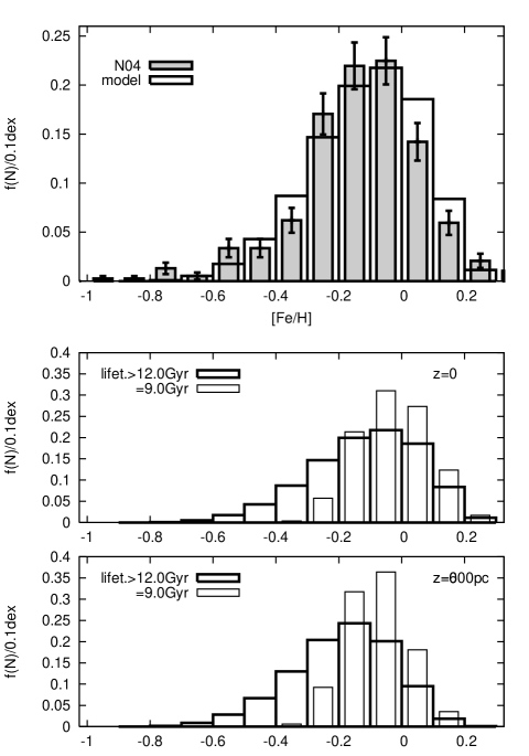
Figure 11: Upper panel: The metal enrichment law for the model (full line). The grey histogram shows the observations from the Copenhagen survey for late G dwarfs in the stellar mass range $0.84\leq M/\rm{M}_{\mathrm{\rm\sun}}\leq 0.90$. Lower panels: The metallicity distribution for early G dwarfs (lifetime 9 Gyr; thin lines) in comparison to the late G, K and M dwarfs (lifetime $>12$ Gyr; thick lines) in the solar neighbourhood and 600 pc above the midplane.

The metal enrichment [Fe/H] and the $SFR$ can be embedded in a local chemical evolution model. We proceed in the following way. We convert the metal abundance [Fe/H] to the oxygen abundance using the correlation of [O/Fe] and [Fe/H] from Reddy et al. (red03 (1993)) by the linear approximation [O/H]=0.375[Fe/H]. For the oxygen enrichment we adopt instantaneous recycling and mixing to determine the infall rate of primordial gas. The mass loss from stellar evolution is taken into account. We start with a negligible initial amount of gas. Then the oxygen yield in solar units is given by $y_{\mathrm{ox}}=\langle Z_{\mathrm{ox}}\rangle+Z_{\mathrm{ox,p}}\Sigma_{\mathrm{g}}/\Sigma_{\mathrm{s}}=1.12$ from the present day surface densities of gas and stars, the present day oxygen abundance $\mathrm{lg}(Z_{\mathrm{ox,p}})=\mathrm{[O/H]_{p}}=0.045$ and the mean oxygen abundance $\langle Z_{\mathrm{ox}}\rangle$ averaged over the star formation history. The infall rate and the surface density of gas and stars are shown in Fig. 1.

4.6 Thick disc

Since the thick disc contributes a few percent to the local density only, its properties are not well determined in the local disc model. Therefore we derive here as an example the density profile of an isothermal thick disc component and discuss the effect on the thin disc. We split the local stellar density into a thin disc and a thick disc component. The local mass fraction of the thick disc is determined to equal the thin disc density at $z\approx 1.2$ kpc as indicated by K dwarf density profiles (Phleps et al. phl05 (2005)). We choose the thick disc velocity dispersion and calculate the complete disc model including the new component. The parameters of all components have to be adjusted iteratively, because the stellar disc profile (thin plus thick disc) has a different shape now. The resultant profiles for thin disc, gas and thick disc using $\sigma_{\mathrm{t}}=41$ km/s and $\rho_{\mathrm{0,t}}=2.6\times 10^{-3}\rm{M}_{\mathrm{\rm\sun}}/\mathrm{pc}^{3}$ corresponding to 6.7% of the local stellar density are shown in Fig. 12 (thick lines). The density profile of the thick disc can be fitted by a sech${}^{\alpha}(z/\alpha h_{\mathrm{t}})$ profile to better than 3%. The corrections of the thin disc parameters due to the thick disc is of the order of 1%. Only the surface density of thin and thick disc is 10% larger with a corresponding reduction of the Dark matter (see Table 2).

Figure 12: Self-consistent isothermal thick disc models with different velocity dispersions. Stars, gas, thick disc 1 form a self-consistent model with parameters ($\sigma_{\mathrm{t}},\rho_{\mathrm{0,t}}/\rho_{\mathrm{0,s+t}},\alpha,h_{\mathrm{t}}$). Velocity dispersion and local mass fraction of the thick disc are input parameter and the power law index and exponential scale height are best fit parameter for a sech${}^{\alpha}(z/\alpha h_{\mathrm{t}})$ profile. For comparison two alternative cooler thick disc components are plotted.

For two alternative models with smaller velocity dispersion of the thick disc the density profiles can also be fitted very well by the sech^α law. The parameters are also given in Fig. 12.

4.7 Initial mass function

For the determination of the IMF from the local luminosity function, the luminosity function is first converted to a mass function $dN=f(M)dM$ using the transformation formulae of Henry & Mc Carthy (hen93 (1993)), corrected in Henry et al. (hen99 (1999)), and extended to bright stars according to Schmidt-Kaler in Landolt-Börnstein (lan82 (1982)). The result is shown in the lower panel of Fig. 13 and compared to the PDMF given in Kroupa et al. (kro93 (1993)). The star numbers are normalized to a sphere with radius R=20 pc. In order to determine the correction factor converting the IMF to the local PDMF due to the finite lifetime and the vertical thickness $h_{\mathrm{ms}}$, the main sequence lifetime is needed. We use the lifetimes estimated from the isochrone evolution shown in Fig. 3 for the different magnitude bins, where the metal enrichment and the relative weighting due to the increasing number of stars with decreasing mass in the mass interval is taken into account. These data are shown in the upper panel of Fig. 13 with a comparison of the lifetimes determined directly from evolutionary tracks of Girardi et al. (gir04 (2004)) and with the analytic fitting formula of Eggleton et al. (egg89 (1989)). Any systematic variation of the lifetimes result in significant corrections to the correction factor and therefore the IMF. This is the most uncertain input to the IMF determination. The correction factors in the solar neighbourhood (z=0 thick line) and for populations above the plane are shown in the middle panel of Fig. 13.

Figure 13: Upper panel: Stellar mass as function of lifetime for the present day population. Symbols are the values used (from Fig. 3), the lines are estimated values from evolution tracks. Middle panel: Correction factor (=IMF/PDMF), which must be applied to the IMF to derive the local star counts of stars with corresponding lifetime relative to low mass stars with lifetime exceeding the disc age. Lower panel: Open circles show the PDMF and the IMF of our sample from CNS4 and Hipparcos. Crosses are the PDMF of Kroupa et al. (kro93 (1993)) and the IMF by correcting with the same dilution factor. The dashed lines are the Scalo IMF and PDMF used in the model and the full lines give the new best fit for the derived IMF (open circles).

The used Scalo IMF (Eq. 26) is consistent with the observed PDMF. But the kink near 1 $\rm{M}_{\mathrm{\rm\sun}}$ seems artificial, because it is near that mass, where the correction factor due to the finite lifetime starts to apply. Therefore we determined a new IMF by fitting power laws in two mass regimes only. The best fit is

$$\mbox{\rm d}N \propto M^{-\alpha}\mbox{\rm d}M\quad\mathrm{with}$$ (37)

$$\alpha=\left\{\begin{array}[]{rcl}1.49\pm 0.09&&0.08\leq M/\rm{M}_{\mathrm{\rm\sun}}<1.61\\ &for&\\ 3.95\pm 0.33&&1.61\leq M/\rm{M}_{\mathrm{\rm\sun}}<6.0\end{array}\right.$$

$$N_{0} = 359/\rm{M}_{\mathrm{\rm\sun}}\quad\mathrm{at}\quad M/\rm{M}_{\mathrm{\rm\sun}}=1.61\,,$$

where $N_{0}$ gives the normalization in the 20 pc sphere. The back-reaction of the corrected IMF to the disc model via the mass loss is very small and not included in the model.

The strongest constraints on the $IMF$ at high masses and the present day $SFR$ is the observed number of A stars in the solar neighbourhood. Since the bright stars with $M_{\mathrm{V}}<0.5$ mag are observed in a sphere with a radius of 200 pc, the sample size is a direct measure of the local surface density. Therefore the conversion from the $IMF$ to the mean $SFR$ in the last few 100 Myr depends only on the lifetime of the stars. That means, a higher present day $SFR$ requires a shorter lifetime for the A stars or an even steeper $IMF$.

The position of the Sun is probably by about 20 pc above the midplane (Humphreys & Larsen hum95 (1995)). The local density of the subpopulations with small scale height are significantly smaller than the midplane density ($M_{\mathrm{V}}<1.5$ mag). We corrected for that implicitly, since we determined the midplane density of these magnitude bins for the PDMF using spheres with large radii (see Table 1), where the offset can be neglected.

5 Summary

We presented an evolutionary disc model for the thin disc in the solar cylinder based on a continuous star formation history (SFR) and a continuous dynamical heating (AVR) of the stellar subpopulations. The vertical distribution of the stellar subpopulations are calculated self-consistently in dynamical equilibrium. The SFR and AVR of the stellar subpopulations are determined by fitting the velocity distribution functions of main sequence stars. A chemical evolution model with reasonable gas infall rate is included, which reproduces the local [Fe/H] distribution of G dwarfs.

We found a vertical disc model for the thin disc including the gas and dark matter component, which is consistent with the local kinematics of main sequence stars and fulfils the known constraints on the surface densities and mass ratios. The SFR shows a maximum 10 Gyr ago declining by a factor of 10 until present time corresponding to an e-folding timescale of 5 Gyr. The velocity dispersion on the upper main sequence depends on the lifetime of the stars, which is derived from the AVR. For the AVR we find a power law with index of 0.375. Applying the stellar lifetime and the new scale height corrections to the PDMF results in a best fit IMF with power-law indices of 1.5 below and 4.0 above 1.6 $\rm{M}_{\mathrm{\rm\sun}}$, which has no kink around 1 $\rm{M}_{\mathrm{\rm\sun}}$.

Including a thick disc component consistently lead to slight variations of the thin disc properties, but a negligible influence on the SFR. A variety of predictions were made concerning the number density, age and metallicity distributions of stellar subpopulations as a function of $z$ above the galactic plane.

References

- (1) Bahcall, J. N., Schmidt, M., Soneira, R. M. 1982, ApJ, 258, L23
- (2) Binney J., Dehnen W., Bertelli G. 2000 MNRAS 318, 658
- (3) Binney J., Tremaine S. 1987, Galactic Dynamics, Princeton Univ. Press, New Jersey
- (4) Bronfman L., Cohen R. S., Alvarez H., May J., Thaddeus P. 1988 ApJ 324, 248
- (5) Cignoni M., Degl’Innocenti S., Prada Moroni P. G., Shore S. N. 2006, A&A 459, 783
- (6) de la Fuente Marcos R., de la Fuente Marcos C. 2004, NewA 9, 475
- (7) Dickey J. M.,Lockman F. J. 1990 ARAA 28, 215
- (8) Eggleton P. P., Fitchett M. J., Tout C. A. 1989, ApJ, 347, 998
- (9) Fioc, M., Rocca-Volmerange, B. 1997, A&A 326, 950
- (10) Girardi L., Grebel E. K., Odenkirchen M., Chiosi C. 2004, A&A 422, 205
- (11) Henry T. J., Mc Carthy D. W. Jr. 1993, AJ 106, 773
- (12) Henry T. J., Franz O. G., Wasserman L. H. L. et al. 1999, ApJ 512, 864
- (13) Hernandez X., Valls-Gabaud D., Gilmore G. 2000 MNRAS, 316, 605
- (14) Holmberg J., Flynn C. 2000 MNRAS, 313, 209
- (15) Holmberg J., Flynn C. 2004 MNRAS, 352, 440
- (16) Humphreys R. M., & Larsen J. A. 1995 AJ 110, 2183
- (17) Jahreiß H., Wielen R. 1997 In B. Battrick, M. A. C. Perryman, eds., Proc. ESA SP-402 (Nordwijk, ESA), 675
- (18) Just A., Fuchs B., Wielen R. 1996 A&A 309, 715
- (19) Just A. 1998 In W. J. Duschl and C. Einsel, eds., ITA Proc. Ser. (Heidelberg, ITA) 2, 119
- (20) Just A. 2001 In S. Deiters, B. Fuchs, A. Just, R. Spurzem, and R. Wielen, eds., ASP Conf. Ser. 228, (star2000), 169
- (21) Kroupa P., Tout C. A., Gilmore G. 1993 MNRAS 262, 545
- (22) Kuiken K., Gilmore G. 1991 ApJ 367, L9
- (23) Lynden-Bell D. 1975 Vistas in Astronomy 19, 299
- (24) Nordström B., Mayor M., Andersen J., et al. 2004 A&A 418, 989
- (25) Phleps S., Drepper S., Meisenheimer K., Fuchs B. 2005 A&A 443, 929
- (26) Reddy B. E., Tomkin, J., Lambert D. L., Allende Prieto C. 2003 MNRAS 340, 304
- (27) Rocca-Pinto H. J., Scalo J., Maciel W. J., Flynn C. 2000, A&A 358, 869
- (28) Robin A. C., Reylé C., Derrière S., Picaud S. 2003 A&A 409, 523
- (29) Scalo J. M. 1986 Fundamentals of Cosmic Physics 11, 1
- (30) Schmidt-Kaler T. 1982 in Landolt-Börnstein Vol. 2, 4.1
- (31) Vyssotsky A. N. 1963 in Basic Astronomical Data, Stars and Stellar Systems 3, 192
- (32) Wilson O., Woolley R. 1970 MNRAS 148, 463
- (33) Wielen R. 1977 A&A 60, 263