Universal scaling of current fluctuations in disordered graphene

Abstract

We analyze the full transport statistics of graphene with smooth disorder at low dopings. First we consider the case of one-dimensional (1D) disorder for which the transmission probability distribution is given analytically in terms of the graphene-specific mean free path. All current cumulants are shown to scale with system parameters (doping, size, disorder strength and correlation length) in an identical fashion for large enough systems. In the case of 2D disorder, numerical evidence is given for the same kind of identical scaling of all current cumulants, so that the ratio of any two such cumulants is universal. Specific universal values are given for the Fano factor, which is smaller than the pseudodiffusive value of ballistic graphene ($F=1/3$) both for 1D ($F\approx 0.243$) and 2D ($F\approx 0.295$) disorders. On the other hand, conductivity in wide samples is shown to grow without saturation as $\sqrt{L}$ and $\log L$ with system length $L$ in the 1D and 2D cases respectively.

I Introduction

Stimulated by the striking results of the first experiments on graphene flakes, Novoselov et al. (2004, 2005); Zhang et al. (2005) interest in the problem of transport in such system has seen extraordinary growth. Castro Neto et al. (2006); Katsnelson (2006); Geim and Novoselov (2007) The particular subject of disorder in graphene has been recently the center of numerous studies, since many of the known concepts and results for transport in disordered normal metals break down for the peculiar dispersion relation of undoped graphene. For example, simple semiclassical techniques fail; Aleiner and Efetov (2006) quantum corrections can show up with opposite sign to the conventional case (weak antilocalization) unless valley symmetry is brokenSuzuura and Ando (2002); McCann et al. (2006); such corrections are conspicuously absent in the cleanest experimental samples, Morozov et al. (2006) the proposed explanation being an effective time-reversal symmetry breaking due to curvature disorder that preserves the valley symmetry in graphene. Morpurgo and Guinea (2006) Indeed, the specific symmetry properties of disorder turn out to be a crucial issue for transport in this system. McCann et al. (2006); Ostrovsky et al. (2006) While atomic-sized defects are widely thought to be of little importance for transport at standard temperatures, Peres et al. (2006); Ziegler (2006); Ostrovsky et al. (2006); Nomura and MacDonald (2007) smooth potentials can have a very visible impact on the conductivity $\sigma$ of graphene. Such electrostatic potentials can arise either from the ubiquitous geometrical corrugation observed Meyer et al. (2007) in most graphene samples, Castro Neto et al. (2006) or from ineffective screening of charges in the environment.Hwang et al. (2007); Galitsky et al. (2007) It has sometimes been dubbed “charge puddle disorder” due to the fact that the gapless nature of graphene makes the material respond to such a potential by forming local particle and hole charge accumulations.Cho and Fuhrer (2007); Katsnelson et al. (2006) Recent measurements Martin et al. (2007) estimate the typical size of charge puddles in the $\xi\sim 10-30\mathrm{nm}$ range, with a typical potential height of $\sigma_{V}\sim 10\mathrm{meV}-100\mathrm{meV}$. Galitsky et al. (2007); Castro Neto and Kim (2007) This gives a typical dimensionless disorder strength $\sigma_{V}\xi/\hbar v_{F}\approx 0.2-2$.

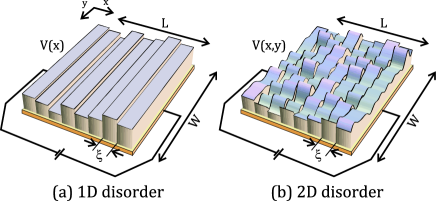
Figure 1: (Color online) Two different disorder realizations considered in this work for a graphene sheet (between metallic contacts) of length $L$ and width $W$. (a) 1D disorder (no mode coupling), (b) model for 2D charge puddle disorder.

The effect of smooth disorder on transport in graphene has been recently analyzed theoretically by a number of authors, Nomura and MacDonald (2007); Titov (2007); Rycerz et al. (2007); Ostrovsky et al. (2007); Bardarson et al. (2007); Nomura et al. (2007); Cheianov et al. (2007) finding once more striking differences with respect to the well known theory of disordered metals. Beenakker (1997) Due to the absence of inter-valley scattering and to chirality conservation, Katsnelson et al. (2006) this kind of disorder has the peculiarity of enhancing the conductivity with respect to the ballistic case, which is at odds with classical intuition. A natural question that arises is whether this enhancement has an upper bound and whether, as a consequence, the conductivity of a large graphene sample exhibits a universal value, as initially claimed, Ostrovsky et al. (2007) or whether it depends on size and system properties, in other words, whether the scaling $\beta(\sigma)$ function in smoothly disordered graphene exists and has fixed points or not. Some of the predictions made so far are conflicting on this point. Using a supersymmetric nonlinear sigma model, Ryu et al. (2007) Ref. Ostrovsky et al., 2007 suggests the existence of a universal minimal conductivity, whereas recent numerical simulations find that $\sigma$ increases in a logarithmic fashion with the system size, Bardarson et al. (2007) while the beta function exists (single parameter scaling) and always remains positive. Nomura et al. (2007); Bardarson et al. (2007) One must bear in mind, however, that the conclusions of Ref. Ostrovsky et al., 2007 rely on a diffusive limit, so that direct comparison to the numerical calculations might not be straightforward. On the other hand, a recent experiment Tan et al. (2007) has shed doubts about the existence of a universal minimal conductivity in real samples.

In this work, we analyze the effect of smooth puddle disorder on the complete transport statistics of graphene at low dopings and, in particular, the scaling properties of current fluctuations with system parameters such as length or disorder strength. First, we study the case of one-dimensional (1D) disorder. We numerically compute transport properties within the transfer matrix formalism. We then derive and solve the single channel Dorokhov-Mello-Pereyra-Kumar (DMPK) equation Mello et al. (1988) for graphene, valid for long samples. The DMPK equation implies that a single parameter scaling for conductivity holds and $\beta(\sigma)=d\log\sigma/d\log L$ exists. Both the analytical solution and the numerical results agree with zero fitting parameters and high accuracy. The most important difference between this result and that of the 1D disordered metal is that in graphene, we find a channel-dependent mean free path that scales quadratically with transverse momentum $q$ for small dopings. The consequence of this in transport for wider-than-long sheets is the peculiar scaling properties of the resulting transmission probability distribution, which we compute analytically. As a consequence of these scaling properties, conductance and all higher current cumulants scale in the same way with system parameters (“universal scaling”), such as system length $L$ or disorder strength. In particular, conductivity is found to grow without saturation as $\sqrt{L}$ with system length, as opposed to the constant conductivity of ballistic graphene. No sign of localization is obtained as expected. The 1D Fano factor is found to saturate, both numerically and analytically, to $F=0.243$.

In the case of two-dimensional (2D) disorder analytical progress is difficult. We numerically calculate the transmission probability distribution, finding that the type of scaling features of the 1D case are also present in two dimenions, albeit with a modified scaling law. Conductivity in wider-than-long 2D samples is found to scale as $\sigma\propto\log L$, like in Ref. Bardarson et al., 2007, without localization, in contrast to the initial suggestions. Ostrovsky et al. (2007) All higher cumulants once more exhibit an identical scaling law as the conductance, leading to truly universal ratios of any pair of cumulants, e.g., $F=0.295$.

The layout of this work is as follows. We first give an overview of the transfer matrix method employed in this work in Sec. II. Then, we study the case of 1D disorder (Sec. III), and give a full analytical solution to its transport statistics at low dopings. The same scaling is found explicitly for all current cumulants in this case. Technical details about the 1D calculation can be found in Appendix B, while a derivation of the DMPK equation in graphene can be found in Appendix A. Motivated by the 1D results, we numerically explore the case of proper 2D disorder in Sec. IV and describe the evidence for universal scaling of current cumulants also in two dimenions. Finally, we conclude in Sec. V.

II Transfer matrix method

Graphene with smooth disorder, which therefore does not couple valleys, can be modeled by a single flavor 2D Dirac Hamiltonian

$$H=v_{F}\bm{\sigma}\cdot\bm{p}+V(x,y)-\epsilon,$$ (1)

where Pauli matrices $\bm{\sigma}$ act on the pseudospin space, $\epsilon$ is the doping, $v_{F}\approx 10^{6}m/s$ is the carrier velocity, $\bm{p}$ is the momentum operator with respect to the Dirac point and $V(x,y)$ is a disorder realization (see Fig. 1). The two valleys and two real spins amount to four degenerate transport channels in this approximation. In the following, all energy scales such as doping $\epsilon$ or potential $V$ will be given in units such that $\hbar v_{F}=1$ for compactness, so that $\epsilon$ will in fact stand for $\epsilon/(\hbar v_{F})$, and so on.

In Refs. Titov, 2007 and Cheianov and Fal’ko, 2006, Titov and Cheianov and Fal’ko derived a differential equation for the transfer matrix $\mathcal{T}_{qq^{\prime}}(L)$ describing the propagation of such Dirac fermions with transverse momenta $q=2\pi n/W$ and energy $\epsilon$ through a graphene sheet of width $W$ and length $L$ under a given realization of disorder $V(x,y)$. In the case of large Fermi wavelength mismatch at the contacts, it takes the formTitov (2007)

$$\frac{d\mathcal{T}_{q^{\prime}q}(x)}{dx} = \sum_{k}\mathcal{M}_{q^{\prime}k}(x)\mathcal{T}_{kq}(x),$$ (2)

$$\mathcal{M}_{q^{\prime}q}(x) = \sigma_{x}\otimes q\,\delta_{q^{\prime}q}+i\sigma_{z}\otimes\left(\epsilon\,\delta_{q^{\prime}q}-V_{q^{\prime}q}(x)\right),$$ (3)

$$V_{q^{\prime}q}(x) = \frac{1}{W}\int_{0}^{W}dyV(x,y)e^{-i(q^{\prime}-q)y}.$$ (4)

The initial condition is $\mathcal{T}(0)=1\!\!1$, and $\delta_{q,q^{\prime}}$ denotes a Kronecker delta. The implicit assumptions in the above equations are that the disorder does not couple valleys (i.e., it is sufficiently smooth), that metallic contacts that connect graphene to the reservoirs are appropriately modeled by infinitely doped graphene ($\epsilon\rightarrow\infty$ for $|x|>L/2$), and that the boundary conditions for the transmission modes can be chosen periodic in the transverse direction. The latter assumption is rigorously valid for $W\gg L$, for which possible boundary-induced pseudospin precession and valley mixing effects can be ignored.

The connection between the transfer and the scattering matrix is given by

$$\mathcal{T}(L)=\left(\begin{array}[]{cc}\hat{t}^{\dagger-1}&\hat{r}^{\prime}\hat{t}^{\prime-1}\\ -\hat{t}^{\prime-1}\hat{r}&t^{\prime-1}\end{array}\right),$$

where $t$ ($r$) are transmission (reflection) amplitude matrices. This allows one to compute eigenvalues $T_{n}$ of the transmission matrix $t^{\dagger}t$, which are conveniently recast into parameters $\lambda_{n}$ through

$$T_{n}=\mbox{sech}^{2}\lambda_{n}\,.$$ (6)

In the context of transport through random disorder $V(x,y)$, one is interested in the probability distribution of the transfer matrix or, more precisely, the distribution $P(\{\lambda_{n}\})$. Within very general assumptions, such distribution was shown to satisfy the DMPK equation Mello et al. (1988) for disordered wires. Beenakker (1997) In the next section, we show that this also applies to graphene with 1D disorder, and we use the known solution to such 1D DMPK equation to compute linear response transport properties.

Given the probability distribution $P(\{\lambda_{n}\})$ for the transmission probabilities, a particularly useful object is the average density distribution $\rho(\lambda)=\sum_{n}\langle\delta(\lambda-\lambda_{n})\rangle$ of the $\lambda_{n}$ above. It allows to compute any current fluctuation average in linear response $\langle C\rangle=\mathrm{Tr}C(\hat{t}^{\dagger}{t})$ by

$$\langle C\rangle=\int_{0}^{\infty}d\lambda\,\rho(\lambda)\,C\left(\mbox{sech}^{2}\lambda\right).$$ (7)

Two particularly interesting cases are the conductivity, for which $C(T)=(4e^{2}/h)(L/W)T$, and the shot noise, $C(T)=(4e^{3}|V|/h)T(1-T)$. In this work, we will also consider the Fano factor, defined as the ratio of disorder averages $F=\langle T(1-T)\rangle/\langle T\rangle$.

III One-dimensional disorder

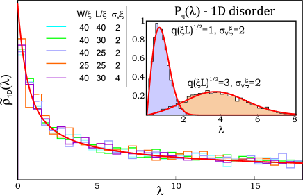
Figure 2: (Color online) Normalized transmission distribution $\rho(\lambda)/\Lambda_{\mathrm{1D}}$ for various 1D disordered undoped graphene systems. Good agreement is found with Eq. (14), plotted in red. Inset: comparison of the distribution [Eq. (9)] to the numerical distribution $P(\lambda_{q})$ for two different values of the transverse momentum $q$. No fitting parameters were used in either case.

We will first use the preceding transfer matrix formalism to study the case of one-dimensional disorder $V(x,y)=V(x)$. In this case, Eq. (4) does not mix modes, which will be labeled by a well defined transversal momentum $q$. The corresponding $\lambda_{q}$ of Eq. (6) will depend on the realization of disorder but will be otherwise mutually independent. If $V(x)$ is further modeled by piecewise constant potential steps of width $\Delta x_{i}$ [see Fig. 1 (a)], it is straightforward to compute the resulting transfer matrix for a given $q$: $\mathcal{T}_{q}(L)=\prod_{i}e^{\mathcal{M}_{qq}(x_{i})\Delta x_{i}}$.

We first use this approach to numerically compute the reduced probability distribution $P(\lambda_{q})$ for a given mode $q$. Random potential realizations are sampled with fixed $\Delta x_{i}=\xi$ (representing the disorder correlation length) and statistically independent Gaussian potentials $V(x_{i})$ of variance $\mbox{Var}[V(x_{i})]=\sigma^{2}_{V}$. Each of these independent potential steps models a 1D version of a charge puddle in graphene. The histogram of the computed transmissions for each realization and mode gives the distribution $P(\lambda_{q})$.

The resulting distribution $P(\lambda_{q})$ for samples of length $L\gg\xi$ (large number of puddles) is rather simple, see inset of Fig. 2. For high transverse momenta $q\sqrt{\xi L}\gg 1$, it evolves into a Gaussian centered at a large $\lambda$, while at lower momenta, it evolves into a Rayleigh-type distribution. Such distribution makes the limit of large number of puddles non-self-averaging, i.e., at low momenta $\langle C(\lambda_{q})\rangle\neq C(\langle\lambda_{q}\rangle)$.

Analytically, one can actually prove that, in the limit of large samples $L\gg\xi$, the distribution $P(\lambda_{q})$ satisfies the single channel DMPK equation for graphene (see Appendix A)

$$l(q)\frac{\partial P}{\partial L}=\frac{1}{4}\frac{\partial}{\partial\lambda_{q}}\left(\frac{\partial P}{\partial\lambda_{q}}-2\coth 2\lambda_{q}P\right),$$ (8)

for a given mode $q$. In general, this equation involves a certain (possibly $q$ dependent) mean free path $l$ to be determined. Its solution is known and is given by Abrikosov (1981); Beenakker (1997)

$$P_{s}(\lambda)=2\sqrt{\frac{2}{\pi}}\frac{e^{-s/4}}{s^{3/2}}\int_{\lambda}^{\infty}du\frac{ue^{-u^{2}/s}\sinh 2\lambda}{\sqrt{\cosh 2u-\cosh 2\lambda}},$$ (9)

where $s=s(q)=L/l(q)$. As a side note, this solution is, for most practical purposes, quite indistinguishable from the simpler Rice distribution, $P_{s}(\lambda)\approx R_{s/2,\sqrt{s/2}}(\lambda)$, defined as

$$R_{\bar{\lambda},\nu}(\lambda)=\frac{1}{\nu^{2}}\exp\left(-\frac{\lambda^{2}+\bar{\lambda}^{2}}{2\nu^{2}}\right)\lambda I_{0}\left(\frac{\lambda\bar{\lambda}}{\nu^{2}}\right).$$ (10)

The DMPK equation does not describe transport through evanescent modes, which are explicitly neglected in its derivation, see Eq. (26). Transport through clean graphene at zero doping, on the other hand, is dominated by evanescent modes. The weak disorder limit of the DMPK solution is therefore quite different from the case of clean graphene, which has $P(\lambda_{q})\approx\delta(\lambda_{q}-qL)$. Tworzydlo et al. (2006) In fact, the validity of the DMPK solution requires long enough samples so that the high $q$ evanescent modes that are unaffected by disorder have died out, while the smaller $|q|<\sqrt{\epsilon^{2}+\sigma_{V}^{4}\xi^{2}}$ modes are converted into propagating modes by the effect of disorder. The ignored evanescent modes have x-wave vector $|k_{x}|>\sigma_{V}^{2}\xi$, so that, more quantitatively, this long sample condition reads $\sigma_{V}^{2}L\xi\gg 1$. The weak disorder limit of the DMPK solution corresponds, therefore, to that in which a single charge puddle has a weak effect on the scattering matrix, $\sigma_{V}\xi\ll 1$, but all of them together have a strong effect $\sigma_{V}^{2}L\xi\gg 1$.

One way to find the correct form of $s(q)$ in Eq. (9) is to directly derive the DMPK equation from Eq. (2). This is done in Appendix A in the case of weak disorder and small doping, $\sigma_{V}\xi,\epsilon\xi\ll 1$. A more powerful way, also applicable to strong disorder, $\sigma_{V}\xi\gtrsim 1$, is to obtain an exact result for some expectation values of a function of $\lambda_{q}$, such as $\langle\cosh 2\lambda_{q}\rangle$. It is possible to compute this average analytically from Eq. (2) in the case of 1D piecewise disorder with a large number of charge puddles, see Appendix B. By comparing it to the same average obtained from the distribution [Eq. (9)], one arrives at the relation

$$s(q) = \frac{1}{2}q^{2}L\xi\gamma,$$ (11)

for $L\gg\xi$ and $\epsilon\xi\ll 1$, where

$$\gamma=\frac{2(\sigma_{V}\xi)^{2}}{(\epsilon\xi)^{2}+(\sigma_{V}\xi)^{4}},$$ (12)

if $\sigma_{V}\xi\ll 1$, $\sigma_{V}^{2}\xi L\gg 1$ (we call this ‘weak disorder’), and

$$\gamma=\frac{(\sigma_{V}\xi)^{2}(2\sqrt{2\pi}\sigma_{V}\xi+\pi-2)-(\epsilon\xi)^{2}(\pi+\sqrt{2\pi}\sigma_{V}\xi)}{2(\sigma_{V}\xi)^{4}},$$ (13)

if $\sigma_{V}\xi\gtrsim 2$ (strong disorder). All the dependence on doping and disorder details is contained in $\gamma$. The derivation of the above expressions for $\gamma$ is valid for piecewise gaussian disorder to second order in the average doping $\epsilon$ and $L\gg\xi$. Note that an identical result is non-trivially obtained if a different average such as $\langle\cosh^{2}2\lambda_{q}\rangle$ is used for the calculation, which indicates that Eq. (9) is not merely an approximation, but is indeed exact for small dopings $\epsilon\xi\ll 1$, both in the strong and weak disorder limits. We conjecture that any other model of 1D smooth-disorder would satisfy, for large enough samples and low dopings, the above power-law equation for $s(q)\propto q^{2}$ with a certain $\gamma$ (independent of $q$ and $L$), regardless of the details of disorder.

Equation (9) is valid for any ratio $W/L$. In the case of wider-than-long graphene sheets, however, the average eigenvalue density function $\rho_{\mathrm{1D}}(\lambda)=\sum_{q}P_{q}(\lambda)$ takes on a remarkably simple form

$$\rho_{\mathrm{1D}}(\lambda) = \sqrt{\frac{2W^{2}}{\pi L\xi\gamma}}\tilde{\rho}_{\mathrm{1D}}(\lambda),$$ (14)

$$\tilde{\rho}_{\mathrm{1D}}(\lambda) = \frac{\rho_{\mathrm{1D}}(\lambda)}{\rho_{\mathrm{1D}}(0)}=\frac{\sqrt{2}}{\pi}\int_{\lambda}^{\infty}\frac{K_{1}(u)\sinh 2\lambda}{\sqrt{\cosh 2u-\cosh 2\lambda}}du,$$

valid in practice for $W\gtrsim L$. Here, $K_{1}(u)$ is the first modified Bessel function of the second kind. Note that for most practical purposes, the simpler function $\tilde{\rho}_{\mathrm{1D}}(\lambda)\approx e^{-\lambda}I_{0}(\lambda)$, where $I_{0}$ is the modified Bessel function of the first kind, can be used to within excellent accuracy. Implicit in the derivation of Eq. (14) is that all modes $-\infty<q<\infty$ are properly described by Eq. (9), which as discussed above is valid if $\sigma_{V}^{2}\xi L\gg 1$.

In Fig. 2, we compare the numerical $\rho_{\mathrm{1D}}(\lambda)$ as obtained by disorder sampling in 1D to the above analytical expression [Eq. (14)] without any fitting parameters, finding a very good agreement, even when $W$ is not much bigger than $L$.

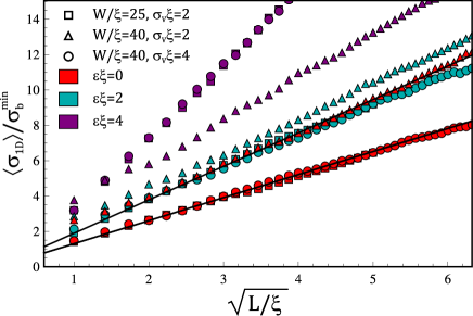
Figure 3: (Color online) Numerical results for the average conductivity vs. system length $L/\xi$ through a graphene sheet with 1D disorder. (Note that data with $L>W$ are not shown.) The results are normalized to the ballistic minimal conductivity $\sigma_{\mathrm{b}}^{\mathrm{min}}=4e^{2}/\pi h$. A $\sigma\propto\sqrt{L/\xi}$ scaling is obtained already from $L\approx\xi$. At low dopings, Eq. (15) -black lines- agrees with the numerical results.

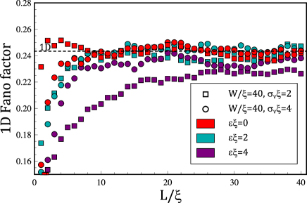
Figure 4: (Color online) Fano factor vs sheet length $L$ for various system parameters and 1D disorder. The saturation value is universal at low dopings (in red) and lies at the value $F=0.243$ derived from Eq. (14).

One of the main features of $\rho_{\mathrm{1D}}$ for graphene with smooth disorder [Eq. (14)] is the absence of a localization length. In other words, conductivity defined as $\sigma\equiv G\frac{L}{W}$ grows indefinitely with system size, scaling as

$$\sigma=0.49\sqrt{\frac{1}{\gamma}}\sqrt{\frac{L}{\xi}}$$ (15)

for large $L/\xi$. A similar scaling in one dimension was found in the case of white noise disorder within an approximate self-averaging assumption.Titov (2007) This is in contrast to the constant $\sigma$ of ballistic graphene Tworzydlo et al. (2006) and to the $\sigma\sim\log L$ scaling behavior observed for 2D disorder by Bardarson et al., Bardarson et al. (2007) as we will discuss in the next section. The $L^{1/2}$ scaling of conductivity is not surprising, however, in view of the property $l(q)\propto q^{-2}$. Indeed, within the window of propagating $q$ modes, those with sizable transmission (ballistic modes) satisfy $l(q)\sim 1/\xi q^{2}\gtrsim L$. Therefore, there will be approximately $W/\sqrt{\xi L}$ such ballistic modes (those with smaller q). These modes will dominate transport, so that one expects the same $\sqrt{1/L}$ scaling for the conductance and hence a conductivity $\sigma\propto\sqrt{L}$.

Another important feature of Eq. (14) is that all the details of the system (disorder strength, size, and doping) enter as a $\lambda$-independent prefactor to the density $\tilde{\rho}_{\mathrm{1D}}(\lambda)$ and do not affect the shape of the density profile. This directly implies that, in the parameter regime of validity for Eq. (14), the ratio of any pair of current cumulants is universal (independent of system size, mean free path, and disorder strength) since all current cumulants will scale with these parameters in the same way as the conductivity. In particular, the Fano factor in the presence of 1D puddle disorder close to the Dirac point becomes $F_{\mathrm{1D}}\approx 0.243$, below the pseudodiffusive prediction $F=1/3$ for ballistic graphene.Tworzydlo et al. (2006) The numerical results for the conductivity and Fano factor in 1D are shown in Figs. 3 and 4, respectively, as a function of system length $L/\xi$. The numerical Fano factor is indeed seen to saturate close to $F=0.243$ independent of system parameters. The average conductivity also scales as $\sqrt{L/\xi}$ at low dopings as expected. Interestingly, this scaling persists also at higher dopings for which the derivation of $s(q)$ [Eq. (11)] ceases to be valid.

IV Two-dimensional disorder

In a realistic model of disordered graphene with $W>L$, mode mixing becomes important, so the preceding discussion of 1D disorder need not apply. Indeed, as mentioned in the Introduction, some authors claimed Ostrovsky et al. (2007) that large graphene sheets would, in fact, reach a universal value of conductivity in the presence of smooth disorder (no intervalley scattering), while others Bardarson et al. (2007) numerically found a nonuniversal conductivity scaling as $\sigma\propto\log L$ for deltalike and Gaussian-correlated 2D disorder potentials. As we will show in this section, our results support the latter nonuniversal conductivity in puddle disordered graphene. In addition, our results suggest the existence of universal ratios of current cumulants in the limit $W\gtrsim L\gg\xi$, just as in the 1D case.

In the presence of mode mixing due to two-dimensional disorder, the transfer matrix technique can still be used for numerical simulations, although it becomes more computationally intensive. Our goal once more is to compute the density $\rho_{\mathrm{2D}}(\lambda)=\sum_{n}P_{n}(\lambda)$ in the presence of charge puddle disorder of typical size $\xi$ in both $x$ and $y$ directions, which we model by a random potential profile $V(x,y)=\sum_{q}a_{q}(x)e^{iqy}$. Harmonics $a_{q}(x)$ are approximated by piecewise constant functions in $x$ at intervals of size $\xi$. For a given $x$, $a_{q}(x)$ is assumed to be Gaussian distributed with variance $\mathrm{Var}[a_{q}(x)]=\sigma_{V}^{2}$ for all $q<2\pi/\xi$. Higher harmonics are suppressed, as expected by the smoothness of charge puddles of typical size $\xi$. The resulting potential, depicted in Fig. 1(b), is convenient for numerical computations [$V_{q^{\prime}q}(x)=a_{q^{\prime}-q}(x)$)] but can still be considered realistic for charge puddle disorder. For practical calculations, a high-momentum cutoff must be introduced; it is chosen high enough so that the result for $\rho_{\mathrm{2D}}(\lambda)$ is cutoff independent. The computation of the transmissions is performed by composition of scattering matrices, rather than by multiplication of transfer matrices, since the latter method is unstable when many modes (higher momenta) have small transmissions, as is the case here.

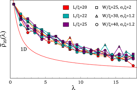
Figure 5: (Color online) Normalized transmission density distribution for 2D disorder and zero doping. For large enough systems, all the curves coincide (within the noise), suggesting a universal scaling for current cumulants just as for 1D disorder (red dotted line).

As can be seen in Fig. 5, the density $\rho_{\mathrm{2D}}(\lambda)$ clearly deviates from the 1D solution (red dotted line). Strikingly, however, the shape of $\rho_{\mathrm{2D}}(\lambda)$, up to a global rescaling factor $\Lambda_{\mathrm{2D}}$ (see below), is clearly independent of the sample length, width, or scattering strength as long as $L/\xi\gg 1$ (complete mode mixing) and $W\gtrsim L$ (continuum of transport momenta). When such conditions are satisfied, the disordered system acquires some universal features. All the dependence of $\rho_{\mathrm{2D}}(\lambda)$ on system parameters $W,L,\xi$, $\sigma_{V}$, and $\epsilon$ appears to enter as a $\lambda$-independent prefactor,

$$\rho_{\mathrm{2D}}(\lambda)\approx\Lambda_{\mathrm{2D}}(L,W,\xi,\sigma_{V},\epsilon)\tilde{\rho}_{\mathrm{2D}}(\lambda),$$ (16)

for some pure function of $\lambda$, $\tilde{\rho}_{\mathrm{2D}}(\lambda)$, just as in the 1D case Eq. (14). It is interesting to compare this pure function, plotted in Fig. 5, to the Dorokhov result Dorokhov (1984); Nazarov (1994) for diffusive metals which is $\lambda$ independent for large samples. Ballistic graphene (zero disorder) also has a $\lambda$-independent $\rho(\lambda)$.

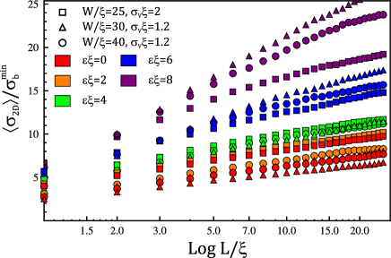
Figure 6: (Color online) Conductivity in 2D disordered graphene for various average dopings $\epsilon$ and system parameters. A clear $\log L$ scaling is observed up to $L\sim W$, where the transition to a quasi-1D ribbon regime begins.

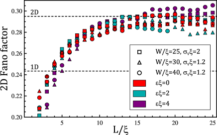
Figure 7: (Color online) As for 1D disorder, the Fano factor saturates to a system independent value, this time around $F=0.295$ for large systems sizes.

Conductance and higher current cumulants are obtained from Eq. (7). In contrast to the 1D case, we see in Fig. 6 that the minimal conductivity $GL/W$ is proportional to $\log L/\xi$, in agreement with Ref. Bardarson et al., 2007. The observed logarithmic dependence of the conductance on the sample size $L$ might be attributed to the weak antilocalization. According to Ref. McCann et al., 2006 (see also Ref. Cheianov et al., 2007), the weak antilocalization correction to the conductance of a 2D disordered graphene in the diffusive regime $L\gg l$, with no intervalley scattering, no magnetic impurities, and no interaction between electrons, should read

$$\delta\sigma\approx\frac{2e^{2}}{\pi^{2}\hbar}\ln\frac{L}{l}\equiv\sigma_{b}^{\min}\ln\frac{L}{l}.$$ (17)

Our low energy numerical data appear to be in reasonable agreement with this expression. At $\epsilon\xi<4$, we find $d\sigma/d\ln L=1.3-1.5\;\sigma_{b}^{\min}$ (see Fig. 6). Unfortunately, we do not know the value of the mean free path $l$ and therefore cannot independently verify if our samples are in the diffusive regime. Most probably, at low energies, we get $l\lesssim L$ and the diffusive model applies, while at higher energies, we have $l\sim L$ which leads to a stronger dependence of the conductance on $L$. Such an interpretation of the results plotted in Fig. 6 suggests that the mean free path $l(\epsilon)$ should grow with energy as it did in case of 1D disorder.

From the logarithmic dependence of the conductivity, it immediately follows that $\Lambda_{\mathrm{2D}}(L,W,\xi,\sigma_{V},\epsilon)\propto\frac{\log(L/\xi)}{L}$. This implies that shot noise and higher current cumulants should all scale with $\frac{\log(L/\xi)}{L}$. This behavior is indeed observed numerically (not shown explicitly), confirming Eq. (16).

Just as in the 1D case, the form of Eq. (16) implies once more that the ratio of any pair of current cumulants will be universal if $L/\xi\gg 1$ and $W\gtrsim L$. The Fano factor, in particular, acquires a universal value $F_{\mathrm{2D}}\approx 0.295$, as can be seen in Fig. 7. Note that $1/3>F_{\mathrm{2D}}>F_{\mathrm{1D}}$.

V Conclusions

In conclusion, we have characterized the full transport statistics of disorder graphene in the absence of intervalley scattering. We have computed numerically the transmission probability distribution both for 1D and 2D disorders. In both the 1D and 2D cases we have found non-self-averaging statistics and no localization length. All current cumulants are seen to grow monotonously with system length without any saturation, which suggests that experimental results for the minimal conductivity should be limited by contact resistance.

In the 1D case, we have shown that the solution for long samples satisfies a single channel DMPK equation, for which we give the exact analytical solution and the expression for the mean free path at low dopings. Such mean free path scales as $l\propto q^{-2}$ with the transverse momentum, which has important consequences for the scaling properties of current cumulants. Such scaling properties, observed numerically also in 2D, suggest that, for long and wide enough samples, all cumulants scale in an identical fashion with system size, leading to universal ratios of any two cumulants. Although the same phenomenon is obtained in the theory of diffusive metals,Nazarov (1994) the resulting transport statistics is less trivial in the case of graphene. The Fano factor in 2D disordered graphene $F=0.295$, for example, is below the value in diffusive metals and clean graphene $F=1/3$.

Appendix A Derivation of the one-dimensional Dorokhov-Mello-Pereyra-Kumar equation for graphene

Following Titov, Titov (2007) we parametrize the $T-$matrix as follows:

$${\cal T}=\left(\begin{array}[]{cc}e^{i\varphi_{1}}\cosh\lambda_{q}&e^{-i\varphi_{2}}\sinh\lambda_{q}\\ e^{i\varphi_{2}}\sinh\lambda_{q}&e^{-i\varphi_{1}}\cosh\lambda_{q}\end{array}\right).$$ (20)

From Eq. (2), we derive the following equations Titov (2007)

$$\frac{d\lambda_{q}}{dx} = q\cos 2\theta_{q},$$ (21)

$$\frac{d\theta_{q}}{dx} = \epsilon-V(x)-q\sin 2\theta_{q}\;\coth 2\lambda_{q},$$ (22)

where $\theta_{q}=(\varphi_{1}-\varphi_{2})/2$. The initial condition for Eqs. (21) and (22) reads $\lambda_{q}(0)=0$ and $\theta_{q}(0)=0$. Our aim is to derive an equation for the averaged distribution function $P(\lambda_{q},\theta_{q})$. We proceed along the standard route and begin with the equation for the non-averaged distribution function $\tilde{P}(\lambda_{q},\theta_{q})=\delta[\lambda_{q}-\lambda_{q}(x)]\delta[\theta_{q}-\theta_{q}(x)]$, where $\lambda_{q}(x),\theta_{q}(x)$ are the solution of Eqs. (21) and (22). This equation reads

$$\frac{\partial\tilde{P}}{\partial x} = -\frac{\partial}{\partial\theta_{q}}\big{(}(\epsilon-V(x)-q\sin 2\theta_{q}\;\coth 2\lambda_{q})\tilde{P}\big{)}$$ (23)

$$-\frac{\partial}{\partial\lambda_{q}}\big{(}q\cos 2\theta_{q}\;\tilde{P}\big{)}.$$

Now we assume that $q\xi,\epsilon\xi,\sigma_{V}\xi\ll 1$. In this case, the fluctuating potential can be treated as $\delta$ correlated, i.e., we consider

$$\langle V(x_{1})V(x_{2})\rangle=\sigma_{V}^{2}\xi\delta(x_{1}-x_{2}).$$ (24)

The averaging over $V(x)$ in Eq. (23) becomes very simple and we arrive at the usual Fokker-Plank equation for $P=\langle\tilde{P}\rangle$:

$$\frac{\partial P}{\partial x} = -\epsilon\frac{\partial P}{\partial\theta_{q}}+\frac{\sigma_{V}^{2}\xi}{2}\frac{\partial^{2}P}{\partial\theta_{q}^{2}}-q\cos 2\theta_{q}\frac{\partial P}{\partial\lambda_{q}}$$ (25)

$$+\,q\coth 2\lambda_{q}\left(2\cos 2\theta_{q}P+\sin 2\theta_{q}\frac{\partial P}{\partial\theta_{q}}\right).$$

Next, we assume

$$q^{2}\lesssim\epsilon^{2}+\sigma_{V}^{4}\xi^{2}.$$ (26)

Then, the isotropization of $P(\lambda_{q},\theta_{q})$ over the angle $\theta_{q}$ happens fast, so that derivatives with respect to $\theta_{q}$ in Eq. (25) are small. We split the distribution $P(\lambda_{q},\theta_{q})$ into the sum of an isotropic part and small anisotropic correction,

$$P(\lambda_{q},\theta_{q})=P(\lambda_{q})+\alpha(\lambda_{q})\cos 2\theta_{q}+\beta(\lambda_{q})\sin 2\theta_{q}.$$ (27)

We derive three coupled equations for $P$, $\alpha$ and $\beta$. To this end, we first average Eq. (25) over the angle $\theta_{q}$, then multiply it with $\cos 2\theta_{q}$ and average the result, and, finally, we multiply Eq. (25) with $\sin 2\theta_{q}$ and average over $\theta_{q}$ again. We then get

$$\frac{\partial P}{\partial x} = -\frac{q}{2}\frac{\partial\alpha}{\partial\lambda_{q}},$$

$$\frac{1}{2}\frac{\partial\alpha}{\partial x} = -\epsilon\beta-\sigma_{V}^{2}\xi\alpha-\frac{q}{2}\frac{\partial P}{\partial\lambda_{q}}+q\coth 2\lambda_{q}\,P,$$

$$\frac{1}{2}\frac{\partial\beta}{\partial x} = \epsilon\alpha-\sigma_{V}^{2}\xi\beta.$$ (28)

Under the condition [Eq. (26)] we can set $\partial\alpha/\partial x=\partial\beta/\partial x=0$. Then $\alpha$ and $\beta$ are easily excluded and we arrive at the one channel DMPK equation

$$l(q)\frac{\partial P}{\partial x}=\frac{1}{4}\frac{\partial}{\partial\lambda_{q}}\left(\frac{\partial P}{\partial\lambda_{q}}-2\coth 2\lambda_{q}P\right),$$ (29)

with the effective mean free path

$$l=\frac{\epsilon^{2}+\sigma_{V}^{4}\xi^{2}}{\sigma_{V}^{2}\xi q^{2}}.$$ (30)

Let us briefly discuss this result. First of all Eq. (A11) predicts an infinite mean free path for an electron moving perpendicular to the potential barriers ($q=0$), i.e. no back-scattering occurs in this case. This is a manifestation of Klein paradox. At finite values of $q$ the momentum of an incident electron is no longer perpendicular to the surface of the barrier, which makes the back-scattering possible. As a result the mean free path (A11) becomes finite. Such behavior of the mean free path is encoded in the mathematical structure of Eqs. (2) and (3). Namely, it is related to the fact that, in the case of 1D disorder, the off-diagonal matrix elements of ${\cal M}_{q^{\prime}q}$, responsible for back-scattering are proportional to $q$. One can actually derive the mean free path (A11) directly from Eqs. (2)-(4) in a simple way. To this end one should assume $q$ to be sufficiently small and treat the off-diagonal elements of the matrix ${\cal M}_{q^{\prime}q}$ perturbatively. Since Eq. (2) is formally similar to the Schrödinger equation for a spin rotating in magnetic field, the ”rate” of back-scattering, which should be identified with $1/2l$ in our problem, is given by a Fermi golden rule like expression

$$\frac{1}{2l}=q^{2}\,{\rm Re}\,\int_{-\infty}^{0}dy\left\langle e^{2i\epsilon(x-y)-2i\int_{y}^{x}dzV(z)}\right\rangle_{V(x)}.$$ (31)

The averaging over the fluctuating potential $V(x)$ with the correlator (24) reduces to the evaluation of a simple gaussian path integral and indeed leads to the expression (30) for the mean free path.

Note that the preceding derivation requires white-noise-like disorder with $\sigma_{V}\xi\ll 1$. We state without proof that, in the limit of strong disorder $\sigma_{V}\xi\gtrsim 2$, Eq. (29) still holds, as is made plausible by the consistent derivation of $s=L/l$ in Appendix B. In this case however, the mean free path has a different form from Eq. (30).

Moreover, the condition (26) implies that the DMPK equation applies only to modes which lie within a window $|q|\lesssim\sqrt{\epsilon^{2}+\sigma_{V}^{4}\xi^{2}}$. All modes with higher $q$ are weakly sensitive to disorder and are, in fact, evanescent. When this window is finite (for finite disorder or finite doping), the evanescent modes can be ignored provided that the sample is long enough. The precise condition is $\sigma_{V}^{2}L\xi\gg 1$. In this limit, the contribution of the evanescent modes with $|q|\gtrsim\sqrt{\epsilon^{2}+\sigma_{V}^{4}\xi^{2}}$ to the conductance is negligible and Eq. (14) becomes valid.

Appendix B Analytical results for one-dimensional disorder averaging

The problem of computing the mean free path $l(q)$ that enters the 1D distribution [Eq. (9)] is tackled here by finding analytical solutions for the expectation value of a certain function of $\lambda$, in our case $\langle\cosh 2\lambda\rangle$, and then adjusting $s=L/l$ in order to recover that same result from the distribution (9). This is done for low dopings and both for the strong and the weak disorder limits. The procedure is carried out also for a different function $\langle\cosh^{2}2\lambda\rangle$, which yields an identical mean free path, which confirms the fact that Eq. (9) is the exact distribution for transmissions through graphene with 1D smooth disorder, as modeled by Eq. (2).

As explained in Ref. Titov, 2007, an alternative form of Eq. (2) for mode $q$ under 1D disorder is given by Eqs. (21) and (22). The dynamics of $\theta$ and $\lambda$ therein is coupled. However, we are interested in expectation values of functions that do not involve $\theta$ (as is the case of any observable current cumulant). The following exact reformulation of Eqs. (21) and (22) proves useful to obtain them:

$$\bm{v}(x) \equiv \left(\begin{array}[]{c}\cosh 2\lambda\\ \sinh 2\lambda\cos 2\theta\\ \sinh 2\lambda\sin 2\theta\end{array}\right),$$ (35)

$${Q}(x) \equiv \left(\begin{array}[]{ccc}0&2q&0\\ 2q&0&-2(\epsilon-V(x))\\ 0&2(\epsilon-V(x))&0\end{array}\right),$$ (39)

$$\frac{d\bm{v}(x)}{dx} = {Q}(x)\bm{v}(x),$$ (40)

with the exact solution

$$\bm{v}(L)=P\exp\left(\int_{0}^{L}{Q}(x)dx\right)\bm{v}(0).$$ (41)

where $P\exp$ stands for a path ordered exponential. With a piecewise potential $V(x)$ in which each step of size $\xi$ is statistically independent of the others, the average $\langle v(L)\rangle$ reads

$$\langle v(L)\rangle=\left[\langle e^{{Q}\xi}\rangle\right]^{L/\xi}\bm{v}(0).$$ (42)

We therefore need to obtain the average of ${U}\equiv e^{{Q}\xi}$ for a single charge puddle. To proceed analytically we have to assume that the average doping $\epsilon$ is small, so we expand ${U}$ to second order in $\epsilon$. We will furthermore assume that the system contains a large number of puddles, $N=L/\xi\gg 1$. In this case, as will become apparent later, it is also sufficient to expand ${U}$ to second order in $q$, since higher orders will not contribute to $\langle U\rangle^{N}$ in the large $N$ limit.

Let us now consider the case of strong disorder, which as it turns out means $\sigma_{V}\xi\gtrsim 2$. After the two previous expansions, ${U}$ can be averaged by using a Gaussian distribution for $V$ with dispersion $\sigma_{V}$. The resulting expression contains terms of the form $\mathrm{Erf}(\sqrt{2}\sigma_{V}\xi)$ and $e^{-2\sigma_{V}^{2}\xi^{2}}$, which can be greatly simplified to $1$ and $0$ respectively in the strong disorder limit $\sigma_{V}\xi\gtrsim 2$. To exponentiate the result one computes the eigenvalues of the resulting $\langle{U}\rangle$. One eigenvalue is zero, another is small as $q^{2}$ and the last one is close to 1, so that if ${D}$ is the matrix that diagonalizes $\langle{U}\rangle$, one can write

$$\left[\langle e^{{Q}\xi}\rangle\right]^{L/\xi}={D}\left(\begin{array}[]{ccc}(1+(q\xi)^{2}\gamma)^{L/\xi}&0&0\\ 0&[(q\xi)^{2}\tilde{\gamma}]^{L/\xi}&0\\ 0&0&0\end{array}\right)D^{-1},$$ (43)

where

$$\gamma = \frac{(\sigma_{V}\xi)^{2}(2\sqrt{2\pi}\sigma_{V}\xi+\pi-2)-(\epsilon\xi)^{2}(\pi+\sqrt{2\pi}\sigma_{V}\xi)}{2(\sigma_{V}\xi)^{4}},$$

$$\tilde{\gamma} = \frac{\pi(\epsilon\xi)^{2}-(\sigma_{V}\xi)^{2}(\pi-2)}{2(\sigma_{V}\xi)^{4}}.$$

In the limit of large number of puddles $N=L/\xi\rightarrow\infty$, we have $[1+(q\xi)^{2}\gamma]^{L/\xi}\rightarrow\exp[q^{2}\xi L\gamma]$, and $[(q\xi)^{2}\tilde{\gamma}]^{L/\xi}\rightarrow 0$, and higher order corrections in $q$ become irrelevant. By writing down the expression for $D$ in leading (zeroth) order in $q$, and selecting the first element of $\langle\bm{v}(L)\rangle$ in Eq. (42), we arrive at

$$\langle\cosh 2\lambda\rangle=\exp\left(q^{2}L\xi\gamma\right).$$ (44)

From this result it becomes clear that $q\xi$ is indeed a small expansion parameter for the relevant momenta, since the typical momentum scale that appears after averaging is $q\sim 1/\sqrt{L\xi}\ll 1/\xi$.

Similarly we can obtain $\langle\cosh^{2}2\lambda\rangle$ by doing an analogous computation for $\bm{v}_{2}(L)\equiv\bm{v}(L)\otimes\bm{v}(L)$, whose equation of motion involves ${Q}\otimes 1\!\!1+1\!\!1\otimes{Q}$ instead of ${Q}$. The result in that case for the first element of $\langle\bm{v}_{2}(L)\rangle$ reads

$$\langle\cosh^{2}2\lambda\rangle=\frac{1}{3}+\frac{2}{3}\exp\left(3q^{2}L\xi\gamma\right).$$ (45)

The above is valid for strong disorder. In the case of weak disorder, we can expand

$$\langle{e}^{{Q}\xi}\rangle^{L/\xi} \equiv \exp\left[\frac{L}{\xi}\log\left(1\!\!1+\langle Q\rangle\xi+\frac{1}{2}\langle Q^{2}\rangle\xi^{2}\right)\right]$$

$$\approx \exp\left\{\frac{L}{\xi}\left[\langle Q\rangle\xi+\frac{1}{2}\xi^{2}(\langle Q^{2}\rangle-\langle Q\rangle^{2})\right]\right\}.$$

Once again, only one of the eigenvalues of the exponent is relevant for the computation of $\langle\cosh 2\lambda\rangle$. In the limit of large $L/\xi$, this eigenvalue reads $q^{2}\xi L\gamma$, where now

$$\gamma=\frac{2(\sigma_{V}\xi)^{2}}{(\epsilon\xi)^{2}+(\sigma_{V}\xi)^{4}},$$

and we again find

$$\langle\cosh 2\lambda\rangle = \exp\left(q^{2}L\xi\gamma\right),$$

$$\langle\cosh^{2}2\lambda\rangle = \frac{1}{3}+\frac{2}{3}\exp\left(3q^{2}L\xi\gamma\right).$$ (46)

The same averages computed from the 1D DMPK distribution [Eq. (9)] read

$$\langle\cosh 2\lambda\rangle = \exp(2s)$$

$$\langle\cosh^{2}2\lambda\rangle = \frac{1}{3}+\frac{2}{3}\exp(6s).$$ (47)

Comparing Eqs. (44)-(47), we get $s=\frac{1}{2}q^{2}L\xi\gamma$, i.e. Eq. (11).

References

- Novoselov et al. (2004) K. S. Novoselov, A. K. Geim, S. V. Morozov, D. Jiang, Y. Zhang, S. V. Dubonos, I. V. Grigorieva, and A. A. Firsov, Science 306, 666 (2004).
- Novoselov et al. (2005) K. S. Novoselov, A. K. Geim, S. V. Morozov, D. Jiang, M. I. Katsnelson, I. V. Grigorieva, S. V. Dubonos, and A. A. Firsov, Nature (London) 438, 197 (2005).
- Zhang et al. (2005) Y. B. Zhang, Y. W. Tan, H. L. Stormer, and P. Kim, Nature (London) 438, 201 (2005).
- Castro Neto et al. (2006) A. H. Castro Neto, F. Guinea, and N. M. Peres, Physics World 19, 33 (2006).
- Katsnelson (2006) M. I. Katsnelson, Materials Today 10, 20 (2006).
- Geim and Novoselov (2007) A. K. Geim and K. S. Novoselov, Nat. Mater. 6, 183 (2007).
- Aleiner and Efetov (2006) I. L. Aleiner and K. B. Efetov, Phys. Rev. Lett. 97, 236801 (2006).
- Suzuura and Ando (2002) H. Suzuura and T. Ando, Phys. Rev. Lett. 89, 266603 (2002).
- McCann et al. (2006) E. McCann, K. Kechedzhi, V. I. Fal’ko, H. Suzuura, T. Ando, and B. L. Altshuler, Phys. Rev. Lett. 97, 146805 (2006).
- Morozov et al. (2006) S. V. Morozov, K. S. Novoselov, M. I. Katsnelson, F. Schedin, L. A. Ponomarenko, D. Jiang, and A. K. Geim, Phys. Rev. Lett. 97, 016801 (2006).
- Morpurgo and Guinea (2006) A. F. Morpurgo and F. Guinea, Phys. Rev. Lett. 97, 196804 (2006).
- Ostrovsky et al. (2006) P. M. Ostrovsky, I. V. Gornyi, and A. D. Mirlin, Phys. Rev. B 74, 235443 (2006).
- Peres et al. (2006) N. M. R. Peres, F. Guinea, and A. H. Castro Neto, Phys. Rev. B 73, 125411 (2006).
- Ziegler (2006) K. Ziegler, Phys. Rev. Lett. 97, 266802 (2006).
- Nomura and MacDonald (2007) K. Nomura and A. H. MacDonald, Phys. Rev. Lett. 98, 076602 (2007).
- Meyer et al. (2007) J. C. Meyer, A. K. Geim, M. I. Katsnelson, K. S. Novoselov, T. J. Booth, and S. Roth, Nature (London) 446, 60 (2007).
- Galitsky et al. (2007) V. M. Galitsky, A. Shaffique, and S. Das Sarma (2007), arXiv:cond-mat/0702117, Phys. Rev. B (to be published).
- Hwang et al. (2007) E. H. Hwang, S. Adam, and S. Das Sarma, Phys. Rev. Lett. 98, 186806 (2007).
- Cho and Fuhrer (2007) S. Cho and M. S. Fuhrer (2007), arXiv:0705.3239.
- Katsnelson et al. (2006) M. I. Katsnelson, K. S. Novoselov, and A. K. Geim, Nat. Phys. 2, 620 (2006).
- Martin et al. (2007) J. Martin, N. Akerman, G. Ulbricht, T. Lohmann, J. H. Smet, K. von Klitzing, and A. Yacoby (2007), arXiv:0705.2180v1.
- Castro Neto and Kim (2007) A. H. Castro Neto and E. A. Kim (2007), arXiv:cond-mat/0702562.
- Ostrovsky et al. (2007) P. M. Ostrovsky, I. V. Gornyi, and A. D. Mirlin, Phys. Rev. Lett. 98, 256801 (2007).
- Bardarson et al. (2007) J. H. Bardarson, J. Tworzydlo, P. W. Brouwer, and C. W. J. Beenakker, Phys. Rev. Lett. 99, 106801 (2007).
- Nomura et al. (2007) K. Nomura, M. Koshino, and S. Ryu (2007), arXiv:0705.1607v1.
- Titov (2007) M. Titov, Europhys. Lett. 79, 17004 (2007).
- Rycerz et al. (2007) A. Rycerz, J. Tworzydlo, and C. W. J. Beenakker, Europhys. Lett. 79, 57003 (2007).
- Cheianov et al. (2007) V. V. Cheianov, V. I. Fal’ko, B. L. Altshuler, and I. L. Aleiner (2007), arXiv:0706.2968v2.
- Beenakker (1997) C. W. J. Beenakker, Rev. Mod. Phys. 69, 731 (1997).
- Ryu et al. (2007) S. Ryu, C. Mudry, H. Obuse, and A. Furusaki, Phys. Rev. Lett. 99, 116601 (2007).
- Tan et al. (2007) Y.-W. Tan, Y. Zhang, K. Bolotin, Y. Zhao, S. Adam, E. Hwang, S. D. Sarma, H. L. Stormer, and P. Kim (2007), arXiv:0707.1807v1.
- Mello et al. (1988) P. A. Mello, P. Pereyra, and N. Kumar, Annals of Physics 181, 290 (1988).
- Cheianov and Fal’ko (2006) V. V. Cheianov and V. I. Fal’ko, Phys. Rev. B 74, 041403(R) (2006).
- Abrikosov (1981) A. A. Abrikosov, Solid State Communications 37, 997 (1981).
- Tworzydlo et al. (2006) J. Tworzydlo, B. Trauzettel, M. Titov, A. Rycerz, and C. W. J. Beenakker, Phys. Rev. Lett. 96, 246802 (2006).
- Dorokhov (1984) O. N. Dorokhov, Solid State Communications 51, 381 (1984).
- Nazarov (1994) Y. V. Nazarov, Phys. Rev. Lett. 73, 134 (1994).