Reachability and recoverability of sink nodes in growing acyclic directed networks

Abstract

We study the growth of networks from a set of isolated ground nodes by the addition of one new node per time step and also of a fixed number of directed edges leading from the new node to randomly selected nodes already in the network. A fixed-width time window is used so that, in general, only nodes that entered the network within the latest window may receive new incoming edges. The resulting directed network is acyclic at all times and allows some of the ground nodes, then called sinks, to be reached from some of the non-ground nodes. We regard such networks as representative of abstract systems of partially ordered constituents, for example in some of the domains related to technological evolution. Two properties of interest are the number of sinks that can be reached from a randomly chosen non-ground node (its reach) and, for a fixed sink, the number of nonoverlapping directed paths through which the sink can be reached, at a given time, from some of the latest nodes to have entered the network. We demonstrate, by means of simulations and also of analytic characterizations, that reaches are distributed according to a power law and that the desired directed paths are expected to occur in very small numbers, perhaps indicating that recovering sinks late in the process of network growth is strongly sensitive to accidental path disruptions.

I Introduction

The study of large, essentially unstructured networks of interacting elements, also referred to as complex networks, has in the past several years received considerable attention. The main motivation behind so much interest has been the realization that networks occurring in many natural, technological, and social domains have common statistical properties that, though governed by strictly local interactions among the networks’ elements, relate globally to the networks’ structure or functionality. A comprehensive collection of papers spanning the main aspects of this emerging discipline, from origins to representative applications, can be found in Bornholdt and Schuster (2003); Newman et al. (2006).

While it seems correct to say that most network models studied so far are undirected, reflecting the fact that the local interactions occur between pairs of interconnected elements in any of the two possible directions (this is the case, for example, of the networks that represent the Internet at some level), there are also several cases in which interactions are inherently unidirectional, as for example the WWW Barabási et al. (2000), networks of bibliographic citations Vazquez , and also networks that arise from certain flows of information in computer networks Stauffer and Barbosa (2006a, b, 2007). Unidirectional interactions give rise to directed networks (that is, networks whose edges have directions), which in turn have been studied for both structural Dorogovtsev et al. (2001); Barbosa et al. (2003, 2004); Bernhardsson and Minnhagen (2006) and functional Kullmann et al. (2002); Grönlund (2004) properties.

The structure of directed networks is considerably more intricate than that of undirected networks, and this is due primarily to the existence of directed cycles, that is, node sequences in which it is possible to return to any node by following edges along their directions. The existence of such cycles in a directed network is strictly necessary for nontrivial strongly connected components to appear, so it comes as no surprise that many of the network’s properties depend on whether directed cycles exist, how large they are, and how they relate to other structures in the network. So, even though some attention has been given to network elements that lie outside directed cycles Morelli (2003) or to how the network looks when directed cycles are broken Costa (2004), a fair appraisal seems to be that studying directed networks has so far concentrated primarily on properties that depend on the existence of directed cycles.

However, we find that a surprising number of systems are naturally representable by directed networks that are intrinsically acyclic, that is, contain no directed cycles (even though plenty of cycles exist if one ignores the edges’ directions). Such networks exist at much more abstract levels than the majority of the networks that have received attention from researchers, reflecting in general the partial order that is inherent to their nature or to the manner in which they are constructed. Important examples are: networks of immediate event precedence, both in history Schweizer (1996) and in the unfolding of distributed computations Lamport (1978); networks of object inheritance in object-oriented programs Tsantalis et al. (2006); the probabilistic graphical models, known as Bayesian networks, that represent the causal relationships among random variables in some artificial-intelligence systems Pearl (1988); networks that represent possible deductions in axiomatic systems of formal proof Carbone (2002); and networks of word etymology in large language groups bab .

Perhaps the reason why systems such as these have not yet been approached from a complex-network perspective is ultimately the elusiveness that they have about them. In some cases, data are simply not readily obtainable, as seems to be the case of the networks that reflect the innards of large software or artificial-intelligence systems. In others, as in the history and etymology systems, even defining the network’s elements depends on data that are no longer extant and thus requires extensive hypothesizing. Even so, it seems possible to postulate some prototypical growth model for acyclic directed networks and then use it in the study of properties that are expected to be of interest.

Our approach in this paper is to study the growth of acyclic directed networks from an initial set of ground nodes by the continual addition of new nodes and directed edges. At each time step, the growth is limited to the addition of one single node and a fixed number of edges outgoing from that node to randomly selected nodes already in the network. We impose a constraint on which are the nodes toward which new edges may be added: as a new node enters the network, the outgoing edges it acquires must necessarily lead to nodes inside a fixed-size window representing that time step’s immediate past. Both finite and infinite windows are considered, so we hope to be contemplating a wide variety of circumstances in regard to the previously mentioned networks as well as others.

Unlike most other studies of complex networks, in the present case the central entities to be observed are not node degrees (distributions are trivially obtainable for both in- and out-degrees, as we discuss shortly), but have to do instead with whether (and from which nodes) the ground nodes remain reachable as time elapses and, if they do, the nature of the directed paths that lead to them. What we have found is that ground-node reachability depends on how the number of ground nodes relates to window size, and also that the number of ground nodes that can be reached is at times distributed as a power law. As for recovering ground nodes from the latest nodes added to the network, this is expected to be achievable only through a very small number of nonoverlapping directed paths, thus indicating high susceptibility to failure should one such path be disrupted.

II The model and basic properties

We study network evolution for discrete time $t\geq 1$ from an initial set of $n_{0}$ isolated ground nodes. One new node is added per time step, so the elapsing of time step $t$ causes the network to have $n_{0}+t$ nodes. We identify the ground nodes by the nonpositive integers $-n_{0}+1,\ldots,0$, thus imposing an arbitrary order on them, even though they are all assumed to be present when network growth begins. We also use $t$, interchangeably, to refer both to time step $t$ and to the node added at that time step. Upon entering the network, node $t$ acquires two outgoing edges leading to distinct nodes chosen randomly from the set $\{\max\{-n_{0}+1,t-w\},\ldots,t-1\}$ for some window $w\geq n_{0}$. If $t\leq w+1$, then this set contains

$$w_{t}=\min\{n_{0},w-t+1\}$$ (1)

ground nodes; it contains no ground nodes otherwise. [Note that the choice of $2$, as opposed to some other constant, as the number of outgoing edges per node added to the network is qualitatively irrelevant, so we make it for simplicity’s sake only. Similarly, we rule out the possibility of $w<n_{0}$, because this is qualitatively equivalent to using a number of ground nodes equal to $w$ (since it implies that $n_{0}-w$ ground nodes are guaranteed to remain isolated indefinitely).]

Every non-ground node has an out-degree of exactly $2$. As for in-degrees, we may concentrate on some non-ground node $i$ and let $k\in\{0,\ldots,w\}$. The probability that $i$ has in-degree $k$ is clearly given by

$${{w}\choose{k}}\left(\frac{2}{w}\right)^{k}\left(1-\frac{2}{w}\right)^{w-k}\approx\frac{2^{k}e^{-2(1-k/w)}}{k!},$$ (2)

which approximates the probability that, at time $t\gg n_{0}$, a randomly chosen node has in-degree $k$. For $k\ll w$, it approaches the mean-$2$ Poisson distribution. (Note that, if we condition on ground nodes exclusively, the in-degree distribution becomes more concentrated at low degrees than the mean-$2$ Poisson, which implies a lower mean value.)

We henceforth refer to every non-isolated node having no outgoing edges as a sink, and to every non-isolated node having no incoming edge as a source. Clearly, every ground node becomes a sink when picked to be directed an edge at for the first time, and conversely only ground nodes may be sinks. Likewise, every non-ground node is a source upon entering the network, though it may cease being one afterward; conversely, no ground node may be a source.

Let $S_{t}$ denote the expected number of sinks just before the addition of node $t$ to the network. We have $S_{1}=0$ and, for $t\geq 1$,

$$S_{t+1}=S_{t}+\Delta_{t},$$ (3)

where $\Delta_{t}$ is the expected number of new sinks created when node $t$ is added. Of the $w_{t}$ ground nodes that may acquire a new incoming edge at time $t$, let those that are already sinks amount to an expected number $f_{t}$. Then $f_{t}=(w_{t}/n_{0})S_{t}$ and $w_{t}-f_{t}=w_{t}(1-S_{t}/n_{0})$.

The number of node pairs from which to choose at time $t$ is $(w_{t}+t-1)(w_{t}+t-2)/2$. Of these, $[w_{t}+t-1-(w_{t}-f_{t})](w_{t}-f_{t})$ are expected to lead to the creation of one new sink, while $(w_{t}-f_{t})(w_{t}-f_{t}-1)/2$ others are expected to lead to the creation of two new sinks. We then obtain

$$\Delta_{t} = \frac{2(w_{t}-f_{t})(f_{t}+t-1)}{(w_{t}+t-1)(w_{t}+t-2)}$$ (4)

$$\hskip 36.135pt\mbox{}+\frac{2(w_{t}-f_{t})(w_{t}-f_{t}-1)}{(w_{t}+t-1)(w_{t}+t-2)}$$

$$= \frac{2w_{t}(1-S_{t}/n_{0})}{w_{t}+t-1}.$$ (5)

Approximating (3) by a differential equation yields two possibilities, depending on $t$. For $1\leq t\leq w+1-n_{0}$, $w_{t}=n_{0}$ and we get

$$\frac{dS_{t}}{dt}+\frac{2S_{t}}{n_{0}+t-1}=\frac{2n_{0}}{n_{0}+t-1},$$ (6)

thence

$$S_{t}=\frac{n_{0}(t-1)(2n_{0}+t-1)}{(n_{0}+t-1)^{2}}$$ (7)

is obtained from $S_{1}=0$. For $w+1-n_{0}\leq t\leq w+1$, $w_{t}=w-t+1$ and we get

$$\frac{dS_{t}}{dt}+\frac{2(w-t+1)S_{t}}{wn_{0}}=\frac{2(w-t+1)}{w},$$ (8)

thence

$$S_{t}=n_{0}\left\{1-\left(\frac{n_{0}}{w}\right)^{2}\exp\left[\left(\sqrt{\frac{w}{n_{0}}}-\frac{t-1}{\sqrt{wn_{0}}}\right)^{2}-\frac{n_{0}}{w}\right]\right\}$$ (9)

results from $S_{w+1-n_{0}}=n_{0}[1-(n_{0}/w)^{2}]$ [cf. (7)]. Notice that expressing $S_{t}/n_{0}$ as a function of $(t-1)/n_{0}$ in (7), which is already independent of $w$, yields a constant with respect to $n_{0}$ as well. Doing the same in (9) reveals an exclusive dependence on the ratio $n_{0}/w$.

Beginning at $t=w+1$, it is no longer possible for any sink to be created, so the expected number of sinks settles at the value, henceforth denoted by $S(n_{0}/w)$, given by

$$S(n_{0}/w)=S_{w+1}=n_{0}\left[1-\left(\frac{n_{0}}{w}\right)^{2}e^{-n_{0}/w}\right],$$ (10)

following (9). For $w=n_{0}$, this becomes $S(1)=n_{0}(1-e^{-1})$, which limits the expected number of sinks at about $63.21\%$ of the ground nodes. As $w$ grows, $S(n_{0}/w)$ approaches $n_{0}$ asymptotically.

Our study on the recoverability of sinks will be based on the nodes that, at time $t$, remain sources inside the latest window (i.e., the window comprising nodes $t-w+1,\ldots,t$). The probability that a node $i$ inside this window remains a source through time $t$ is $[(w-2)/w]^{t-i}$. The expected number of sources inside the latest window, denoted by $R$, is then

$$R=\sum_{i=t-w+1}^{t}\left(\frac{w-2}{w}\right)^{t-i}\approx w\left(\frac{1-e^{-2}}{2}\right),$$ (11)

amounting therefore to roughly $43.23\%$ of the nodes inside the window.

III Reachability and recoverability of sinks

III.1 Reachability

At time $t$, we say that a ground node is reachable from one of the $n_{0}+t$ nodes of the network when a directed path exists between them leading to the ground node. All ground nodes are reachable from themselves, but only sinks are reachable from non-ground nodes. The reach of a node is the number of ground nodes that are reachable from it. A node has unit reach if and only if it is a ground node, and the reach of a non-ground node refers to sinks exclusively.

Let $P_{t}(r)$ be the probability that, at time $t$, a randomly chosen node has reach $r$. Clearly,

$$P_{t}(1)=\frac{n_{0}}{n_{0}+t}.$$ (12)

For $r>1$, however, we expect the number of sinks in the network to play a role in defining the value of $P_{t}(r)$.

As a node enters the network and connects out to two previously existing nodes, its reach has to account for every sink that is reachable from either of those two nodes. In the relatively early stages of network formation, and for sufficiently large $n_{0}$, it is likely that no sink is reachable from the two nodes concomitantly, and in this case the new node’s reach is simply the sum of their reaches. This becomes progressively less likely later on in the evolution of the network, thus making accurate predictions of $P_{t}(r)$ very difficult.

Our finds regarding $P_{t}(r)$ are summarized in Figure 1, whose part (a) refers to $w=n_{0}$. In this case we see that, initially, non-unit reaches tend to be distributed exponentially. For $t=w=n_{0}$, in particular, the exponential character of the distribution is very clear [cf. the inset in part (a) of the figure] and may be expressed as

$$P_{n_{0}}(r)\approx\left(\frac{S(1)}{2n_{0}}\right)a^{r}=\left(\frac{1-e^{-1}}{2}\right)a^{r},$$ (13)

for some constant $a$ such that $0<a<1$. Since the exponential seems to hold across all pertinent reach values, we can find $a$ by requiring

$$P_{n_{0}}(1)+\sum_{r\geq 2}P_{n_{0}}(r)=\frac{1}{2}+\left(\frac{1-e^{-1}}{2}\right)\sum_{r\geq 2}a^{r}=1,$$ (14)

which leads to $a\approx 0.6958$. It also seems that an exponential approximation continues to hold for somewhat larger values of $t$. For $t\gg w$, though, we expect more and more nodes of reach around $S(1)$ to appear, owing to the finiteness of $w$. This is indeed what happens, but aside from this effect we have also found that the passage of time leads the initial exponential approximation to $P_{t}(r)$ to gradually become

$$P_{t}(r)\approx\left(\frac{S(1)}{n_{0}+t}\right)r^{-1}=\left(\frac{n_{0}(1-e^{-1})}{n_{0}+t}\right)r^{-1},$$ (15)

similar therefore to the power law known as Zipf’s law.

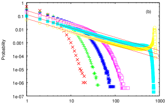
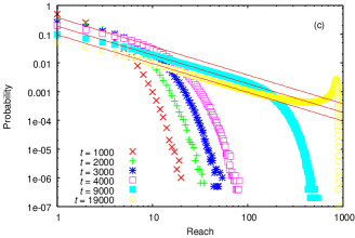
Figure 1: (Color online) Reach distribution for $n_{0}=1\,000$, with $w=n_{0}$ (a), $w=2n_{0}$ (b), and $w=3n_{0}$ (c). Solid lines give the analytic predictions of (13) and (15) for part (a), of (16) for parts (b) and (c). All simulation data are averages over $500$ independent runs.

As we increase $w$ beyond $n_{0}$ to $w=2n_{0}$ and $w=3n_{0}$, we obtain a similar evolution of $P_{t}(r)$ with respect to $t$, including the progressive probability accumulation around $r=S(1/2)$ or $r=S(1/3)$, depending on the case. This is illustrated, respectively, in parts (b) and (c) of Figure 1, where we see that the power-law regime is established only for increasingly larger values of $t$. When this happens, a good approximation to $P_{t}(r)$ seems to be

$$P_{t}(r)\approx\left(\frac{S(1)}{n_{0}+t}\right)\frac{r^{-1}}{n_{0}/w}=\left(\frac{w(1-e^{-1})}{n_{0}+t}\right)r^{-1},$$ (16)

where, curiously, it is still $S(1)$ [not $S(1/2)$ or $S(1/3)$, as we might expect] that drives the distribution, after the simple scaling by $n_{0}/w$.

III.2 Recoverability

We now examine the network’s structure as it relates to the existence of directed paths from the sources in $\{t-w+1,\ldots,t\}$, at time $t$, to the sinks. While the average number of distinct paths over all such source-sink pairs is distributed quite widely, when we look at paths that are not merely distinct but edge-disjoint the situation is very different. For a given source and a given sink, a group of directed paths between them is edge-disjoint if no two paths in the group have any edges in common. The appropriate framework in which to compute the maximum number of edge-disjoint directed paths between two nodes is that of network flows.

Given a directed network with nonnegative numbers associated with the edges (the edges’ capacities), and assuming that it has at least one source and one sink, the maximum flow from a source to a sink is an assignment of numbers to the edges (their flows) such that: no edge flow exceeds the edge’s capacity; the total flow coming into any node equals that leaving the node (except for the source and the sink); and moreover no other assignment results in a greater net flow coming into the sink. By a well-known result from the theory of network flows (the max-flow min-cut theorem), the number of edge-disjoint directed paths from the source to the sink is precisely the maximum flow from the source to the sink under unit capacities Ahuja et al. (1993).

In our present context, the number of edge-disjoint directed paths from any given source to any given sink is at most the minimum between the source’s out-degree (equal to $2$) and the sink’s in-degree (distributed, as we have noted, such that the mean is less than $2$). So we know, beforehand, that the expected average number of such paths, taken over all source-sink pairs of interest, lies somewhere in the interval $[0,2]$. Computing this number is expected to require $RS(n_{0}/w)$ maximum-flow computations for each network. We have used the publicly available, efficient HIPR code of Goldberg for $n_{0}=1\,000$ and three different values of $w$.

For $w=n_{0}$, we have found from $10$ independent runs that the expected average is $0.5024$ at $t=4\,000$, growing to the roughly stable value of $1.2402$ at $t=9\,000$. For $w=2n_{0}$ and $w=3n_{0}$, stabilization occurs later. For $t=4\,000$ and $t=19\,000$, the expected averages are, respectively, as follows: $0.0316$ and $1.4598$ for $w=2n_{0}$, $0.0122$ and $1.5069$ for $w=3n_{0}$. A small increase is then observed at stability as $w$ becomes larger.

Another pertinent indicator of the recoverability of sinks from sources in the latest window at time $t$ is the number of edge-disjoint directed paths from any of the sources to a given sink. Clearly, the expected average number of such paths, taken over all sinks, is some number in the interval $[0,2R]$, since the expected number of sources is $R$ and each has the potential of contributing two paths. However, the sink’s in-degree remains distributed with a less-than-$2$ mean, so it is very unlikely for an expected average significantly larger than $2$ to turn up. As for calculating the desired number of paths in a given network for a given sink, we note that, unlike the preceding case, a little artifice is needed before a maximum-flow computation can be performed (since it is unclear what the source is in such a computation). What we do is to add another source to the network and make capacity-$2$ directed edges outgo from it to all original sources. The combined number of edge-disjoint directed paths from the original sources to the sink is the maximum flow from the new source to the sink. For each network, we expect $S(n_{0}/w)$ maximum-flow computations to be needed.

Results for this second indicator are shown in Figure 2 for $w=n_{0}$ in the main plot set, $w=2n_{0}$ in the top inset, and $w=3n_{0}$ in the bottom inset. The resulting expected values are roughly stable at $t=9\,000$ and equal, respectively, $1.4036$, $1.8192$, and $2.2983$. It is clear from the figure that, for $w=n_{0}$, it is the distribution of the sinks’ in-degrees that exerts the greater influence on how the average number of edge-disjoint directed paths from all sources to one sink is distributed. For $w=3n_{0}$, it is the distribution of the non-sink nodes’ in-degrees (the mean-$2$ Poisson) that eventually does it.

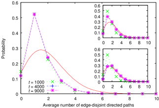
Figure 2: (Color online) Distribution of the average number of edge-disjoint directed paths from all sources to one sink for $n_{0}=1\,000$, with $w=n_{0}$, $w=2n_{0}$ (top inset), and $w=3n_{0}$ (bottom inset). Solid lines give the mean-$2$ Poisson distribution. All simulation data are averages over $500$ independent runs.

IV The case of an infinite window

At time $t$, any value of $w$ surpassing $n_{0}+t-1$ has the effect of an infinite window; that is, any node in the network may be chosen to receive one of the two new edges as an incoming edge. When this is the case, none of our conclusions so far remains valid. Even though the case of infinite $w$ is of little general interest for modeling real systems (it is inherently dependent on global properties of the system as a new node comes in), we feel it is worth commenting on the resulting reach distribution, which differs strikingly from the finite case [except when $r=1$, since $P_{t}(1)=n_{0}/(n_{0}+t)$ remains of course valid].

Expressing $P_{t}(r)$ analytically seems infeasible for most values of $r>1$, but it can be done for $r=2$ and, interestingly, this leads directly to a good approximation for the general case, provided $t\lessapprox 9n_{0}$. Notice first that, for sufficiently large $n_{0}$,

$$P_{t}(2) \approx \left(\frac{1}{n_{0}+t}\right)\sum_{i=1}^{t}\left(\frac{n_{0}}{n_{0}+i-1}\right)^{2}$$ (17)

$$= P_{t}(1)n_{0}\zeta_{t}(2,n_{0}),$$ (18)

where

$$\zeta_{t}(2,n_{0})=\sum_{u=0}^{t-1}\frac{1}{(n_{0}+u)^{2}}$$ (19)

is the truncation, to $t$ terms, of $\zeta(2,n_{0})$, Riemann’s two-parameter zeta function Gradshteyn and Ryzhik (2000). Our heuristic generalization for all values of $r$ is then simply the exponential

$$P_{t}(r)\approx P_{t}(1)\left[n_{0}\zeta_{t}(2,n_{0})\right]^{r-1}.$$ (20)

Simulation results are shown in Figure 3, indicating that, for an infinite window, reach probabilities fall at least as fast as exponentially.

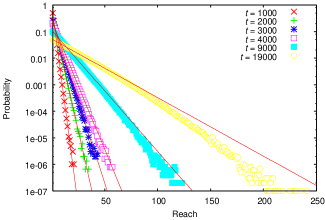
Figure 3: (Color online) Reach distribution for $n_{0}=1\,000$ under an infinite window. Solid lines give the analytic predictions of (20). All simulation data are averages over $500$ independent runs.

V Discussion and concluding remarks

We have considered directed networks that grow from a fixed set of ground nodes by the addition of one node per time step and of two edges directed from that node to previously existing, randomly chosen nodes inside a fixed-length sliding window. Networks thus constructed are devoid of directed cycles, and may be viewed as a prototypical representation of growing collections of partially ordered items, so long as some underlying time-like notion exists with respect to which the window mechanism makes sense. Laying down more than two edges per time step is expected to have no qualitatively significant effect (although it is unlikely for reaches of small even value to exist in the case of three edges, for example—a reach of $2$ is in fact impossible—and therefore reach distributions can be expected to undergo a sort of bifurcation as one moves from high reaches to lower).

Our study has been centered on the two notions that we deem especially relevant for the systems acyclic directed networks are purported to relate to. The first one is the property, here referred to as reachability, of nodes in the network to be able to reach ground nodes via directed paths. We found, by means of simulations and also through limited analytic predictions, that the number of ground nodes reachable from a randomly chosen non-ground node is distributed first exponentially, then as a power law as time elapses. The other notion on which we focused can be summarized as that of how to recover a specific ground node, in the sense of having edge-disjoint directed paths to get to it from some of the latest nodes to be added to the network. Our finds are that such paths are expected to occur in very small numbers on average (roughly somewhere near $2$), and therefore the recoverability of ground nodes may be severely affected by accidental path disruptions.

We believe this paper’s network model, along with its main observables, opens up new possibilities of investigation about abstract systems that are naturally representable as acyclic directed networks. Earlier we mentioned examples from fields related to computer software, artificial intelligence, mathematical logic, and also history. In addition to their being representable as networks such as the ones we studied, what these systems also have in common once viewed from the perspectives of ground-item reachability and recoverability is that many of them make reference, albeit indirectly, to the growing stack of digital technologies that currently separates “ground” pieces of information from their representations for end use. Concerns related to this issue are sometimes voiced in the media, referring, for example, to the digitization of documents une or to a future in which, as some envisage, autonomous systems may become inscrutable regarding their internal organization itw . Even though such issues may seem like a far cry from the study we have pursued in this paper, carrying on with an eye on them may well prove worthwhile.