Choice of Measurement Sets in Qubit Tomography

Abstract

Optimal generalized measurements for state estimation are well understood. However, practical quantum state tomography is typically performed using a fixed set of projective measurements and the question of how to choose these measurements has been largely unexplored in the literature. In this work we develop theoretical asymptotic bounds for the average fidelity of pure qubit tomography using measurement sets whose axes correspond to vertices of Platonic solids. We also present complete simulations of maximum likelihood tomography for mixed qubit states using the Platonic solid measurements. We show that overcomplete measurement sets can be used to improve the accuracy of tomographic reconstructions.

I Introduction and Background

Quantum tomography Vogel and Risken (1989), the practical estimation of quantum states through the measurement of large numbers of copies, is of fundamental importance in the study of quantum mechanics. With the emergence of quantum information science, the tomographic reconstruction of finite dimensional systems Leonhardt (1995) has also become an essential technology for characterizing the experimental performance of practical quantum gates and state preparation. Examples include tomography of the polarization states of light White et al. (1999); Langford et al. (2004) and electronic states of trapped ions Haeffner et al. (2005); Reichle et al. (2006). These experiments would benefit from a systematic study of the optimal measurement and state estimation strategy to use.

There has been much theoretical work in this area, and optimal bounds on state estimation, and constructions for measurements that achieve these bounds are known Holevo (1982); Massar and Popescu (1995); Derka et al. (1998); Vidal et al. (1999); Latorre et al. (1998). These bounds require all copies of the state to be collected and a combined measurement performed across all the copies. While these collective measurements are known to be more powerful than performing measurements on each copy one at a time (local measurements) Massar and Popescu (1995), they are currently totally impractical.

Qubit tomography is currently done using fixed local projective measurements James et al. (2001); Paris and Rehacek (2004). The important question of which fixed local projective measurement sets to use remains an open problem, although there are several relevant theoretical discussions Jones (1991); Bagan et al. (2005); Gill and Massar (2002); Bagan et al. (2006); Rehacek et al. (2004); Roy and Scott (2007). In practice, measurement sets with the minimal number of measurements such as those described in James et al. (2001) have become popular, particularly in optical experiments (but see Langford et al. (2004)). This situation arises since in optical experiments a significant amount of time can be spent on changing the measurement settings. However, such choices are made without much quantitative understanding of how the performance of the tomographic reconstruction is affected by restricting the measurement sets in this way.

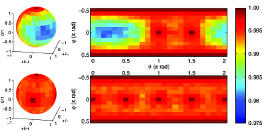
In this paper we investigate how choice of measurements affects the quality of tomographic reconstruction. We follow Jones Jones (1991) and investigate a class of measurement sets based on Platonic solids that provide excellent performance for tomography using fixed local projective measurements. This class of measurement sets allows one to trade off performance against the number of measurement settings, with more overcomplete measurement sets performing better. For example in Fig. 1 we show that both the average and worst case fidelities of the tomographic reconstruction are greatly improved by replacing the popular minimal measurement set of James et al. (2001) with the overcomplete cube Platonic measurement set.

Figure 1: Performance of tomographically reconstructed states on the Bloch sphere for two measurement sets. The top set is a popular set of measurements (James4) used in the literature James et al. (2001), the bottom set is a more isotropic set composed of measurements along the three spatial axes (a cube measurement set), see text for details. For each target state the average fidelity with 400 reconstructed states is plotted by color. The ensemble of reconstructed states was generated by adding Posssonian noise to a simulated experiment with a total of 4000 counts, and then performing maximum-likelihood tomography.

Platonic solid measurements were first proposed for tomography in Jones (1991) for the special case of pure states and using mutual information as a figure of merit. However, this figure of merit makes it hard to compare these results to more recent work which typically uses the average fidelity. We derive new asymptotic bounds for the performance of Platonic solid measurements for pure states using average fidelity as a figure of merit. We then present full numerical simulations of both one and two-qubit tomography performance as a function of the number of copies of the system, using these measurement sets. This provides a detailed study of how information is acquired during a tomography experiment. To our knowledge such a study has not been performed in experimental work but would determine whether tomographic reconstructions are limited by the expected statistics or by other experimental imperfections, such as drifting sources.

The average fidelity is the most commonly used measure of the performance of state reconstruction consequently we make use of this figure of merit. Much of the original interest in fidelity arises from the fact that it bounds the distinguishability of quantum states, see Fuchs (1996). Recently a true quantum Chernoff bound on the distinguishability of states has become available Audenaert et al. (2007) and this quantity is a tighter bound than the fidelity. As a result we use this quantity as figure of merit also, although the results do not depend greatly on this choice.

Very recently, Roy and Scott Roy and Scott (2007) identified a class of measurements, including all the Platonic solid measurements, that give the optimal performance for another figure of merit, the mean squared Hilbert-Schmidt distance. Nevertheless, it will turn out that when average fidelity is used as the figure of merit, there is a range of performance within the class, with the higher order Platonic solids performing better. This indicates that the choice of figure of merit can certainly have a qualitative effect on the comparison between tomographic procedures.

The structure of the paper is as follows: We will introduce the tomography problem, and discuss figures of merit for tomography schemes in section II. In section III we define the Platonic solid measurements. In section IV we describe some other measurement sets that have been studied in the literature for comparison with the Platonic solid measurements. We present theoretical pure state asymptotic bounds on the average fidelity of the tomographic reconstruction for the different platonic solid measurements in section V. We then give some intuition for mixed state tomography in section VI. After presenting details of our mixed state simulations for atomic and photonic qubit systems in section VII we give our results for one and two qubit systems in section VIII. Finally we will investigate the effects of using different figures of merit in sections IX and X.

II Qubit Tomography

A $d$ dimensional quantum state $\rho$ is represented by a $d{\times}d$ positive semidefinite density matrix, with trace one. There are $d^{2}{-}1$ real parameters to be estimated. In the case of optical experiments such as White et al. (1999); Langford et al. (2004) the flux must also be estimated giving $d^{2}$ real parameters to estimate.

Any setting $l$ of an experimental apparatus designed to measure the quantum state may be described by a positive operator value measure (POVM). Each of the $k$ outcomes of a measurement setting is represented by a positive semidefinite operator $O_{lk}$. The operators satisfy $\sum_{k}O_{lk}=I$. The probability of observing outcome $k$ is given by the Born rule $p_{lk}=\mathrm{tr}(\rho\,O_{lk})$. In state tomography each of the $l$ measurements are performed on a large number of copies and estimates obtained for each of the $p_{lk}$. We denote these estimates $\hat{p}_{lk}$. When the number of linearly independent $O_{lk}$ equals or exceeds the number of parameters to estimate, our measurements are known as informationally complete Caves et al. (2002). If these probability estimates were perfect, so that $\hat{p}_{lk}=p_{lk}$, it would be possible to reconstruct the state exactly. In this case there is a set of operators $R_{lk}$, known as a dual basis or dual frame, such that $\rho=\sum_{lk}p_{lk}R_{lk}$. (When the number of linearly independent $O_{lk}$ exceeds the number of parameters to be estimated the dual frame is not unique.) Since our probability estimates are not perfect due to the finite sample size, they may well be inconsistent with any such reconstruction. In this case it is common practise to resort to a maximum likelihood estimate of the state James et al. (2001); Paris and Rehacek (2004). We look at maximum likelihood reconstruction in detail in section VII.3

To judge the quality of reconstruction we need a measure of similarity between the true state $\rho$ and the reconstructed state $\hat{\rho}$. In this paper we will concentrate on two measures. The first is the commonly used fidelity:

$$f(\rho,\hat{\rho}) = \left[\mathrm{tr}\sqrt{\sqrt{\hat{\rho}}\rho\sqrt{\hat{\rho}}}\right]^{2}.$$ (1)

where $0\leq f(\rho,\hat{\rho})\leq 1$ and $f=1$ implies $\rho=\hat{\rho}$. The second is the quantity that determines the recently derived quantum Chernoff bound Audenaert et al. (2007):

$$\lambda_{cb}(\rho,\hat{\rho})=\underset{0\leq s\leq 1}{\mathrm{min}}\mathrm{tr}[\rho^{s}\hat{\rho}^{1-s}].$$ (2)

where as for the fidelity, $0\leq\lambda_{cb}(\rho,\hat{\rho})\leq 1$ and $\lambda_{cb}=1$ also implies $\rho=\hat{\rho}$.

The quantum Chernoff bound has a clear physical interpretation that can be understood by considering the following situation. Suppose an experimentalist wishes to determine if her state preparation device creates the state $\rho$ or the state $\sigma$. Time is limited and she only has $N$ identically prepared copies of the state to work with. She is assumed to be able to perform any measurement, including a collective measurement, in her efforts to distinguish the two states. The result of Audenaert et al. (2007) is that the probability of her making an error is asymptotically $\mathrm{P_{e}}\approx e^{N\ln\lambda_{cb}(\rho,\sigma)}$ where $\lambda_{cb}$ is called the quantum Chernoff bound. When one of the states is pure, the quantum Chernoff bound coincides with the fidelity. Also the square root of the fidelity is always an upper bound on the quantum Chernoff bound. Fuchs (1996); Audenaert et al. (2007). Somewhat confusingly this quantity has also been termed the fidelity in other works and serves as an alternative measure of distinguishability. We have chosen the definition in (1) for it’s appealing interpretation when one of the states is pure, and because all of the theoretical results we mention are derived using this definition. As the quantum Chernoff bound has a clear physical interpretation even when both states are mixed, we consider it a better motivated measure of the distinguishability of $\rho$ and $\sigma$.

Next we define quantities which rate the performance of a tomography scheme for a particular true state $\rho$, using the fidelity and quantum Chernoff bound. The figure of merit we adopt is based on how distinguishable the true state is from the reconstructed state, when averaged over measurement outcomes and an appropriate ensemble of true states. (An interesting alternative approach was advocated by Blume-Kohout and Hayden Blume-Kohout and Hayden (2006).) A tomography experiment produces a list of outcomes of measurements performed on $N$ copies of the true state $\rho$. These outcomes are used to obtain an estimate of the state $\hat{\rho}$, and the fidelity (or quantum Chernoff bound) between the true and estimated states is calculated. Averaging over the outcomes of many such tomography experiments we obtain the point fidelity

$$F(\rho,N)=\sum_{\hat{\rho}}p_{\rho}(\hat{\rho})f(\rho,\hat{\rho})$$ (3)

where $p_{\rho}(\hat{\rho})$ is the probability of estimating state $\hat{\rho}$ given the true state $\rho$. Or point Chernoff bound:

$$\lambda_{pt}(\rho,N)=\sum_{\hat{\rho}}p_{\rho}(\hat{\rho})\lambda_{cb}(\rho,\hat{\rho}).$$ (4)

Finally averaging the point fidelity (or point Chernoff bound) over all possible true states, we obtain the average fidelity:

$$F=\int\!\!d\rho\;F(\rho,N).$$ (5)

or the average Chernoff bound:

$$\lambda_{av}=\int\!\!d\rho\;\lambda_{pt}(\rho,N).$$ (6)

These are the figures of merit we will use to rate a tomography scheme.

To perform the averages over true states in equations (5) and (6), we must choose a prior probability distribution over true states. For pure states there is one clear choice — the Haar measure. For mixed states the choice is not so clear, see for example Zyczkowski and Sommers (2001). We will make use of two priors, one based on the fidelity, and the other on the quantum Chernoff bound.

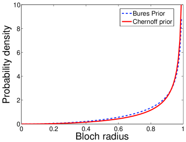
The first, known as the Bures prior, is the density of states induced by defining a volume element using the distance $1/2\arccos f(\rho,\rho+d\rho)$. It is a natural choice when using the fidelity as our measure of similarity between states. It has also been argued that the Bures prior corresponds to maximal randomness of the input states Hall (1998). The Bures prior is unitarily invariant, and it gives a radial probability density on the Bloch sphere:

$$p_{B}(r)=\frac{4}{\pi}\frac{r^{2}}{\sqrt{1-r^{2}}}$$ (7)

When the quantum Chernoff bound is used as the measure of similarity, it is natural to use a prior over states based on this. The natural metric induced by the quantum Chernoff bound was derived in Audenaert et al. (2007). Some of the authors of Audenaert et al. (2007) have also derived the corresponding volume element in the space of states which can be used as a prior on mixed states Munoz-Tapia (2007). In Appendix B we present our general derivation for states of arbitrary dimension. The resulting Chernoff prior is unitarily invariant and the probability density over eigenvalues is given by:

$$p(\lambda_{1}..\lambda_{M})=\frac{C}{\sqrt{\lambda_{1}..\lambda_{M}}}\prod_{k<j}\frac{(\lambda_{k}-\lambda_{j})^{2}}{(\sqrt{\lambda_{j}}+\sqrt{\lambda_{k}})^{2}}$$ (8)

where the eigenvalues are also constrained to satisfy $\sum_{j=1}^{M}\lambda_{j}=1$, and C is a normalisation constant. For single qubit states this corresponds to a radial probability density on the Bloch sphere given by:

$$p_{CB}(r)=\frac{2}{\pi-2}\frac{1-\sqrt{1-r^{2}}}{\sqrt{1-r^{2}}}.$$ (9)

A comparison of the density of the Bures and Chernoff priors is given in Fig. 2. Both these priors have increasing density with state purity. The Chernoff prior is slightly more skewed towards pure states, than the Bures prior.

We will present all of our mixed state results in terms of average fidelity with states drawn according to the Bures prior first, as this has become the popular way of assessing mixed state tomography. We will then present our detailed results using the average Chernoff bound figure of merit with states drawn according to the Chernoff prior. We believe that this figure of merit is better motivated and thus it is important check that our qualitative conclusions do not depend on this choice of figure of merit.

In other works the mean square Hilbert-Schmidt distance and the mean squared Euclidean distance between Bloch vectors have been used as a figures of merit for tomography Scott (2006); Rehacek et al. (2004). For single qubits these measures are equivalent up to constant factors. The Hilbert-Schmidt distance is defined as $D_{\mathrm{hs}}(\rho,\sigma)=\sqrt{\mathrm{tr}(A^{\dagger}A)}$ ,where $A=\rho-\sigma$. It is again related to the probability of error when an experimentalist must determine if she has a state $\rho$ or state $\sigma$, however in this case the experimentalist has only a single copy to measure. Under the assumption that both states are equally likely before the measurement, the probability of error in distinguishing single qubit states $\rho$ and $\sigma$ is $P_{e}=\frac{1}{2}-\frac{1}{2\sqrt{2}}D_{\mathrm{hs}}(\rho,\sigma)$. In order to get an analytically tractable measure of distinguishability Scott (2006); Rehacek et al. (2004) square $D_{\mathrm{hs}}$ before averaging this quantity over measurement outcomes and states as we have done for fidelity and the quantum Chernoff bound. This figure of merit makes it possible to find the optimal measurement sets analytically but after squaring and averaging this quantity is not as well motivated. We will examine the effect of using this figure of merit in section X and show that it can lead to qualitatively different behaviour.

Figure 2: Plot of probability density against Bloch radius for the Bures and Chernoff priors over states. Both distributions have densities which increase with state purity. The Chernoff prior is slightly more skewed towards the pure states than the Bures prior.

III Platonic solid measurements

The state density matrix of a qubit can be written as:

$$\rho=\frac{I+\vec{r}.\vec{\sigma}}{2}$$ (10)

where $\vec{r}$ is a real three dimensional vector known as the Bloch vector, and $\vec{\sigma}$ is a vector of the Pauli matrices $\sigma_{x}$, $\sigma_{y}$ and $\sigma_{z}$. In the special case of pure states, the Bloch vector is unit length. A two-outcome local projective measurement on the $l$th measurement setting can be represented by two projectors:

$$O(\pm\vec{m_{l}})=\frac{I\pm\vec{m_{l}}.\vec{\sigma}}{2}$$ (11)

where $\vec{m_{l}}$ is a real three dimensional unit Bloch vector. The orthogonal outcomes correspond to opposite directions on the Bloch sphere.

As states are isotropically arranged in the Bloch ball, one intuitively expects tomography performance to depend on how isotropically spaced our measurement vectors are on the Bloch sphere. This intuition was supported (and made precise) by the asymptotic pure state results of Jones (1991), and is demonstrated in Fig. 1. In this paper we will concentrate on the measurement sets whose Bloch vectors form Platonic solids. These are the five convex regular polyhedra: tetrahedron, cube, octahedron, dodecahedron and icosahedron. Such shapes are highly isotropic and thus would be expected to give excellent tomographic performance.

Mathematically, the idea of isotropically spacing points on a sphere is also captured by the concept of a spherical $t$-design. A description of $t$-designs is beyond the scope of this paper but note that the properties of $t$-designs mean that they are excellent sets of points for performing numerical estimation of integrals over the sphere with the quality of the approximation being expected to improve as $t$ is increased. This suggests that good measurement sets for tomography may well be associated with $t$-designs. In fact, popular measurement sets for tomography of general quantum systems include the so-called symmetric informationally complete POVMs SicPOVMs Renes et al. (2004) which are spherical 2-designs. We note that the tetrahedron measurement set described below is the SicPOVM for a single qubit, and all the Platonic solids are also 2-designs. In fact it is well known Hardin and Sloane (1996) that the cube and octagon are 3-designs and the dodecahedron and icosahedron are 5-designs. (Note that a $t$-design is also a $t^{\prime}$-design for all $t^{\prime}{<}t$). This further motivates us to concentrate on the performance of the Platonic solids.

There are two possible ways of defining Platonic measurement sets. We define a Platonic solid measurement set to be a set of $L$ different measurement settings whose $2L$ Bloch vectors $\pm\vec{m_{1}}\dots\pm\vec{m_{L}}$ match the $2L$ centres of the faces of a Platonic solid. We use this definition so that an octagon has eight measurement directions. An alternative definition would be to define the Platonic solid measurement as the set of Bloch vectors matching the vertices of a Platonic solid. This definition would result in the same set of shapes because the centres of the faces of one Platonic solid, match the vertices of another Platonic solid. Such solids are said to be duals of each other. The dual pairs are the tetrahedron with itself, the cube with the octagon and the dodecahedron with the icosahedron. We find the first definition more appealing and use it throughout the paper.

The experiments we will be modelling are described in detail in section VII. In the atomic qubit experiment, and the dual-detector photonic experiment each measurement has two orthogonal outcomes. These correspond to opposite directions on the Bloch sphere. Thus two opposite directions are measured simultaneously by a single measurement. All the Platonic solids except the tetrahedron have a face opposite every face and thus these Platonic solid measurements can be measured in this way while the tetrahedron cannot. (Attempting to measure the tetrahedron directions would result in us measuring the octagon instead). For the single-detector photonic qubit experimental model, we will require $L$ measurement settings to obtain the $L$ outcomes, as the orthogonal outcome is not detected. This enables a tetrahedron measurement to be meaningfully measured in this case. Direct measurement of the tetrahedron is possible in principle and schemes have been proposed Decker et al. (2004); Englert et al. (2005), that would however require significantly greater experimental resources so we will not consider this possibility in the following.

We will also be interested in two qubit states. The experimentally simplest measurements are projective measurements performed locally on both subsystems (recording joint outcome probabilities). While we would expect measurement sets that include measurements entangled across both subsystems to give improved results, these measurements are difficult to perform. We will examine the performance of Platonic solid measurements on each subsystem. That is measurements of the form:

$$O(\pm\vec{m_{i}})\otimes O(\pm\vec{m_{j}})$$ (12)

where both $i$ and $j$ range over the $L$ measurements of the same Platonic solid.

IV Measurement sets for comparison

For simulations of one and two qubit optical experiments (single-detector configuration) we will compare our results to the popular measurement sets described in James et al. (2001). The one qubit state measurement set consists of measuring polarizations { H, V, D, R }, that is the horizontal and vertical linear polarizations, the diagonal linear polarization [$\mbox{$|D\rangle$}{=}(\mbox{$|H\rangle$}{+}\mbox{$|V\rangle$})/\sqrt{2}$], and the right circular polarization [$\mbox{$|R\rangle$}{=}(\mbox{$|H\rangle$}{+}i\mbox{$|V\rangle$})/\sqrt{2}$]. We refer to this measurement set as James4. The two qubit state measurement set is { HH, HV, VV, VH, RH, RV, DV, DH, DR, DD, RD, HD, VD, VL, HL, RL } where for example the measurement setting HL means measuring horizontal polarization on the first qubit subsystem and left circular polarization [$\mbox{$|L\rangle$}{=}(\mbox{$|H\rangle$}{-}i\mbox{$|V\rangle$})/\sqrt{2}$] on the second qubit subsystems . We refer to this measurement set as James16. (Notice that this measurement set does not form complete POVMs. The implementation we have in mind is explained fully in Section VII)

In the case of two qubits we also consider a modified version of the SicPOVM of Renes et al. (2004) for comparison. We call this measurement a projective SicPOVM. The original SicPOVM for two qubit states, is an entangled measurement in which a single measurement produces one of 16 outcomes. Experimentally this measurement is difficult to realize. Our projective SicPOVM is a measurement set of 16 settings, in which each setting projects onto one of the directions of the SicPOVM. While still entangled this measurement should be simpler to implement experimentally than the SicPOVM.

V Pure state estimation of qubits with Platonic solids

The bound on average fidelity for collective measurements is known to be: $F{\leq}(N{+}1)/(N{+}2)\approx 1{-}1/N$ where the approximation is good for large $N$. In fact this bound is achievable with collective measurements Massar and Popescu (1995). When restricted to local measurements, measuring the three orthogonal axes of the Bloch sphere (a cube measurement) is known to give an average fidelity bounded by $F{\leq}1{-}13/(12N)$ and again this bound is achievable Bagan et al. (2002). We have derived average fidelity bounds for the other Platonic solids. The derivation only slightly generalizes Appendix B of Bagan et al. (2005). We give an overview of our derivation here, leaving the details to Appendix A.

These bounds on average tomography performance are a consequence of the Cramér-Rao bound of classical statistics. The Cramér-Rao bound concerns the problem of sampling from a probability distribution, where the probability distribution is determined by some parameters. The goal is to estimate these parameters based on the results of sampling the distribution. The Cramér-Rao bound states that the variance of an unbiassed estimator is asymptotically lower bounded by $O(1/N)$, and the coefficient of this scaling is given by the Fisher information (the definition may be found in Appendix A).

In a tomography experiment, with a fixed set of measurements, the outcome probability distribution is fixed by the parameters of the quantum state we are trying to estimate, and we can directly apply the Cramér-Rao bound. The procedure is as follows:

1. Consider a tomography experiment on a quantum state with parameters $\eta$, and its fidelity to the state estimated from the tomographic reconstruction with parameters $\hat{\eta}$. In an asymptotic regime our estimates will be close to the true state, so we can expand the fidelity in a Taylor series about the true state.

2. Calculating the expected value of the fidelity over the different measurement outcomes, we obtain an asymptotic expression for the point fidelity which is a function of the covariance matrix of the estimated parameters.

3. By applying the Cramér-Rao bound to the covariance matrix of the estimated parameters, we can obtain an upper bound on the point fidelity which is a function only of the number of each kind of measurement we have made, and the state parameters.

4. Finally by averaging this point fidelity expression uniformly over the state parameters (using the Haar measure) we obtain the average fidelity bound.

While our expressions are analytic up to the final step, we use numerical integration to average over the state parameters using the Haar measure and obtain our final asymptotic results.

We find $F{\leq}1{-}y/N$ where $y$ is 1.083 for the cube (in agreement with the value of 13/12 in Bagan et al. (2002)), 1.049 for the octahedron, 1.018 for the dodecahedron, and 1.008 for the icosahedron. It is well known in classical statistics that the Cramér-Rao bound can be achieved using a maximum likelihood estimator. Hence the above bounds are also tight. These results show that for pure states the performance of the Platonic solids measurements in tomography is close to the collective measurement bound of $y{=}1$.

Recall that the quantum Chernoff bound is equal to the fidelity if one of the states involved is pure. When, as here, both states are pure the HilbertSchmidt distance is also an equivalent measure as, $D_{hs}^{2}{=}(1{-}f)/2$. So that the choice of figure of merit does not affect the results of this section at all.

VI Mixed state qubit tomography

When the state to be reconstructed can be mixed an analytical treatment is more complicated since the requirement that the density matrix be positive semidefinite leads to constraints on the allowed set of parameters. The situation is also complicated by the way in which the fidelity function depends on the mixedness of the state to be reconstructed. We partially address both these issues in this section, with the main aim to develop intuition. For quantitative results we will resort to simulation.

For mixed state qubit tomography, the state Bloch vector is no longer unit length. The state vector is now:

$$\vec{r}=[r_{x},r_{y},r_{z}]^{T}$$ (13)

where $r_{x}{=}r\cos(\phi)\sin(\theta)$, $r_{y}{=}r\sin(\phi)\sin(\theta)$, $r_{z}{=}r\cos(\theta)$ and $r$ satisfies $r{\leq}1$. This constraint on the length of the Bloch vector reflects the requirement that the density matrix is positive semidefinite.

Mixed state tomography introduces two new complications which we discuss in this section. Both concern behaviour close to the boundary of the Bloch sphere. The first is due solely to the definition of the mixed state fidelity function:

$$f(\vec{r},\vec{\hat{r}})=\frac{1+\vec{r}.\vec{\hat{r}}+\sqrt{1-r^{2}}\sqrt{1-\hat{r}^{2}}}{2}.$$ (14)

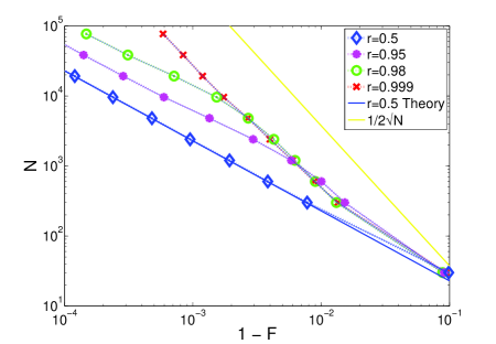
where $\vec{\hat{r}}$ is the estimated state vector. It can be understood by considering only errors in the Bloch vector length $r$ Bagan et al. (2006). Suppose $r{=}1{-}\delta$ and our estimate is $\hat{r}{=}r{-}\epsilon$. Then provided $\epsilon{\ll}\delta$ and both are small we find: $F{\approx}1{-}\epsilon^{2}/8$. From the statistical arguments of the previous section we would expect $\epsilon$ to scale asymptotically like $1/\sqrt{N}$, so we expect to see all point fidelities (except for perfectly pure states) to scale like $F{\approx}1{-}1/8N$ once $N$ is large enough that our errors are well inside the Bloch ball. Alternatively if $\delta{\ll}\epsilon$, we find that the point fidelities scale like $F{\approx}1{-}\epsilon/2$. Thus the general behaviour of point fidelities is a transition from $1/\sqrt{N}$ scaling at low $N$ to a scaling of $1/N$ at large $N$. The transition takes place when the error associated with the state reconstruction $\epsilon$ becomes small enough that $\hat{r}+\epsilon$ lies inside the Bloch ball. Thus the location of the transition happens at higher $N$ for higher purity states. This is illustrated in Fig. 3 where numerical simulations of point fidelities for states with different radial parameters are shown. The Bures prior has a radial distribution that is strongly peaked at $r=1$ and it turns out that when point fidelities are averaged over this prior the $1/\sqrt{N}$ dependence of the point fidelity persists long enough that the dependence of the average fidelity on $N$ is not $N^{-1}$ but rather $N^{-3/4}$ E. Bagan and Rodriguez (2004).

Figure 3: Numerical simulations of atomic point fidelities for a state rotated 45 degrees about the x-axis from the +ve z-axis are plotted against radius on the Bloch sphere. The cube measurement set was used for these simulations. Observe mixed states always have a $1/N$ scaling. States that are close to pure start (after we get to a sufficiently large $N$ to obtain a sensible state estimate) with a $1/\sqrt{N}$ dependence and transition to $1/N$ scaling with larger $N$. This knee occurs at larger $N$ for purer states. Also the statistical theory of equation (15) is plotted for $r{=}0.5$ giving excellent agreement

The second complication arises since our estimated physical state has to be positive semidefinite. For qubits this is equivalent to $\hat{r}{\leq}1$. An estimator that predicts states lying outside the boundary of the Bloch ball can be improved by mapping these states onto the boundary of the Bloch ball which always moves the estimate closer to the true state. Maximum likelihood estimation is a specific example of an estimator that does exactly this. This procedure creates a biassed estimator that nevertheless performs better than any unbiassed one. The naïve Cramér-Rao estimation is therefore not appropriate.

For states well away from the boundary, we can ignore this positivity constraint, and use the unbiased statistical methods of the previous section extended to three parameters to calculate the cube measurement point fidelity:

$$F(\vec{r},N)\leq 1-\frac{3}{4N}\frac{3-3r^{2}+2(r_{y}^{2}r_{x}^{2}+r_{z}^{2}r_{x}^{2}+r_{z}^{2}r_{y}^{2})}{1-r^{2}}.$$ (15)

This value is included in Fig. 3 for the case when $r{=}0.5$ and found to give excellent agreement with the numerical simulations.

VII Simulation details

The main result of this paper is the numerical simulation of tomography using Platonic solid measurements. The simulations are performed in the following way.

1. Choose $N_{s}$ states $\rho_{i}$ at random according to the Bures (or Chernoff) prior. For our simulations $N_{s}$ was chosen to be 10,000.

2. For each $\rho_{i}$, simulate measurements on $N_{c}$ copies of the state (divided equally between the measurement sets) generating $N_{c}$ measurement outcomes $\chi_{i}^{j}$. For our simulations we chose $N_{c}{=}100{,}000$.

3. Perform maximum-likelihood state estimation based on increasing numbers $N$ of these $\chi_{i}^{1}..\chi_{i}^{N}$ obtaining state estimates $\hat{\rho}_{i}(N)$.

4. Calculate the fidelity $f(\hat{\rho}_{i}(N),\rho_{i})$ [or Chernoff bound $\lambda_{cb}(\hat{\rho}_{i}(N),\rho_{i})$] between each state estimate and true state.

5. Calculate the average fidelity $F(N){=}\sum_{i=1}^{N_{s}}f(\hat{\rho}_{i}(N),\rho_{i})/N_{s}$ [or the average Chernoff bound: $\lambda_{av}(N){=}\sum_{i=1}^{N_{s}}\lambda_{cb}(\hat{\rho}_{i}(N),\rho_{i})/N_{s}$].

The Monte-Carlo averaging over states and measurement outcomes is performed simultaneously.

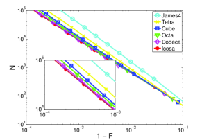
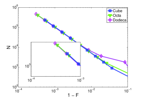
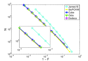
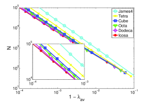
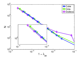
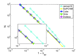
We present our results on a log-log plot of number of copies required against $1{-}F(N)$. To find the number of copies required to achieve a target average fidelity, one can select the target average fidelity on the horizontal axis, and tracing vertically upward, find the number of copies required to achieve that target average fidelity. The inserts on the graphs are enlargements of the largest $N$ section of the graph. The width of the lines on these inserts are approximately equal to the one standard deviation statistical error in average fidelity due to our choice of $N_{s}$.

We simulate two main scenarios, tomography on atomic qubits, and tomography on photonic qubits.

VII.1 Atomic Qubits

The kind of experiment we model here is an atomic qubit as in experiments on trapped ions, such as Haeffner et al. (2005); Reichle et al. (2006) represented by two metastable energy levels $|0\rangle$ and $|1\rangle$, and an auxiliary level $|r\rangle$ used for performing the measurement with a laser driving the transition $\mbox{$|0\rangle$}{\rightarrow}\mbox{$|r\rangle$}$ leading to fluorescence if the state was initially in $|0\rangle$ Cirac et al. (2002). Arbitrary single qubit projective measurements are made available by a first laser pulse tuned to the $\mbox{$|0\rangle$}{\rightarrow}\mbox{$|1\rangle$}$ transition followed by turning a laser on the $\mbox{$|0\rangle$}{\rightarrow}\mbox{$|r\rangle$}$ transition and looking for this fluorescence. We assume the dominant source of error is statistical fluctuation due to the finite number of copies of the state, and neglect all other sources of error. Many of these could be taken into account by replacing our projective measurements with suitable POVMs. However the effects such as drifts in either state preparation or measurement settings would necessitate a different approach.

In this limit these single qubit system measurements are well described by Eqns. (10), (11) and counts for each outcome $k$ of a measurement setting $l$ drawn from a multinomial distribution:

$$p(n_{l1}..n_{lK})=\frac{N_{l}}{n_{l1}..n_{lK}}p_{l1}^{n_{l1}}p_{l1}^{n_{l2}}...p_{lK}^{n_{lK}}$$ (16)

where $N_{l}$ copies of the system are measured with measurement setting $l$, $p_{lk}{=}\mathrm{tr}(\rho O_{lk})$ and $K$ is number of possible outcomes for the measurement (2 for qubit systems and 4 for two-qubit systems).

For two-qubit systems, the measurement operators $O_{lk}$ take the form of Eq. (12) and now the index $l$ ranges over all combinations of single qubit measurement settings on the subsystems. Experimentally this corresponds to noting the joint probability of the four possible outcomes of fluorescence and no fluorescence in each subsystem, for all combinations of measurement settings on the subsystems.

VII.2 Photonic qubits

Figure 4: The single photonic qubit experimental configuration consists of a quarter wave plate and a half wave plate to set the basis, and a polarizing beam splitter followed by a photon detector to analyse in that basis. We call this a single-detector configuration. An additional detector can be placed on the reflected port in a dual-detector configuration, in which case the statistics of the counts can be easily reduced to the atomic case by waiting until a fixed number of counts are obtained for each basis setting.

Our model for experiments on single photonic qubits is shown in Fig. 4. In this model our qubits are represented by the polarization state of photons issuing from a source with Poissonian arrival times. There are two configurations to consider: a single-detector configuration and a dual-detector configuration.

In the first configuration, the source is directed through a quarter wave plate, a half wave plate and polarizing beam splitter (or vertical polarizer) and finally a single photon counter James et al. (2001). The angles of the fast axes of both of the wave plates can be rotated, allowing the projection onto vertical polarization fixed by the final polarizer to be rotated into any polarization state that the experimenter requires. Photon counts are accumulated over a time $t$ for each measurement setting $m_{l}$. The total photons incident on the measurement apparatus during this time is drawn from the Poisson distribution:

$$p(N_{l})=\frac{e^{-\mathcal{N}_{f}t}(\mathcal{N}_{f}t)^{N_{l}}}{N_{l}!}$$ (17)

where $\mathcal{N}_{f}$ is the mean photon flux. The number of these photons reaching the detector $n_{l}$ is then drawn from a binomial distribution with probability $p_{l}=\mathrm{tr}(\rho O_{l})$. The flux is estimated from a set of $r$ measurements satisfying

$$\sum_{i=1}^{r}O_{i}=I$$ (18)

via

$$\mathcal{N}_{f}=\sum_{i=1}^{r}n_{i}/t.$$ (19)

For the Platonic solid measurements, the four measurements of the tetrahedron satisfy (18) and for higher order Platonic solids each axis has two measurements satisfying (18). In the later case an average is made over all the axes to obtain an improved flux estimate.

Adding a detector on the reflected port of the polarizing beam splitter gives a dual-detector configuration and potentially better flux estimation. In this configuration both orthogonal directions are measured simultaneously, and the total flux is estimated by summing the two detector counts. By waiting until a set number of total counts are obtained for each measurement set, the statistics of the counts will reduce to the atomic case covered above.

We also simulate two photon state tomography. A source produces photon pairs whose arrivals are again Poisson distributed according (17). The single photon configuration (single- and dual-detectors) are duplicated (giving two and four detectors). Now only coincidences are counted between the two single photon configurations. The number of co-incidences are drawn from the multinomial distribution of (16). For the single-detector configuration for each qubit we estimate the flux via

$$\mathcal{N}_{f}=\frac{\sum_{j=1}^{r}\sum_{i=1}^{r}n_{ij}}{r^{2}t/4}.$$ (20)

VII.3 Maximum likelihood state reconstruction

After simulating measurements on all copies of the state we have $n_{lk}$ detections corresponding to each measurement operator $O_{lk}$. Maximum likelihood reconstruction is the problem of finding the state $\rho$ which maximizes the likelihood $p(...n_{lk}...|\rho)$ or equivalently minimizes $-\log p(...n_{lk}...|\rho)$. To make our inversions efficiently solvable, we convert (an approximate version of) this problem into a semidefinite program.

For atomic (single and multiple) qubit systems, and for each measurement setting $l$, the outcomes follow the multinomial distribution of (16).

We will approximate these statistics with a Gaussian distribution with mean $\mu_{lk}{=}p_{lk}(\rho)N_{l}$ and a covariance matrix $V_{l}$ with diagonal entries $(V_{l})_{ii}{=}N_{l}p^{e}_{li}(1{-}p^{e}_{li})$, and off-diagonal entries $(V_{l})_{ij}{=}-N_{l}p^{e}_{li}p^{e}_{lj}$ where $p^{e}_{lk}{=}n_{lk}/N_{l}$. Since the outcomes of different measurement settings are statistically independent, the combined likelihood function is $p(...n_{lk}...|\rho){=}\prod_{l}p(n_{l1}..n_{lK})$. Defining $\vec{n_{l}}$ as the vector with $k$th element $n_{lk}$, and $\vec{\mu_{l}}$ as the vector with $k$th element $\mu_{lk}$, our approximate problem is to find a state $\rho$ which minimises

$$-\log p(...n_{lk}...|\rho)\propto\sum_{l}(\vec{n_{l}}-\vec{\mu_{l}})^{T}V_{l}^{-1}(\vec{n_{l}}-\vec{\mu_{l}})$$ (21)

We have assumed that the term in the exponential of the Gaussian dominates the likelihood and used experimental probabilities $p^{e}_{lk}$ instead of $p_{lk}(\rho)$ in the covariance matrices $V_{l}$ to make the problem convex. This enables the problem to be converted into a semidefinite program and solved with the SeDuMi semidefinite program solver software Sturn .

For the dual-detector simulations of single photon and two photon experiments the maximum likelihood reconstruction is identical to the reconstruction for the atomic case (if we wait for a fixed number of counts).

For single-detector simulations of single photon and two photon experiments, the counts are Poisson distributed and as we only measure one outcome per measurement setting, all outcomes are statistically independent. We make a Gaussian approximation with the expected number of counts for measurement outcome $O_{l}$ equal to the variance in those counts i.e. $\mu_{l}{=}\sigma_{l}^{2}{=}\mathcal{N}_{l}{=}p_{l}\mathcal{N}_{f}t$ where $p_{l}{=}\mathrm{tr}(\rho O_{l})$. Our approximate problem is to find the state $\rho$ which minimise the log likelihood

$$-\log[p(n_{1},n_{2},...|\rho)] = \sum_{l}\frac{(n_{l}-\mathcal{N}_{l})^{2}}{2\mathcal{N}_{l}}$$

$$= \frac{\mathcal{N}_{f}t}{2}\sum_{l}\frac{(p^{\mathrm{e}}_{l}-p_{l}(\rho))^{2}}{p_{l}(\rho)},$$

where $p^{\mathrm{e}}_{l}=n_{l}/(\mathcal{N}_{f}t)$. In this case we were able to use $\mathcal{N}_{l}$ for mean and variance without losing the convexity of the problem.

VIII Results

VIII.1 Single atomic qubit results

(a) 1 atomic qubit	(c) 1 photonic qubit
(b) 2 atomic qubits	(d) 2 photonic qubits

Figure 5: Tomography simulation results with a Bures prior. The plot is the number of copies of the state against $1{-}F$ where $F$ is the average fidelity. To read, select the desired average fidelity on the horizontal axis, and trace vertically to find the number of copies of the state required to achieve that fidelity. Each plot shows the performance of various Platonic solids. Tomography for: (a) single atomic qubit states. The tetrahedron can not be measured in this configuration. (b) two atomic qubit states. (c) single photonic qubit with single-detector configuration. (d) two photonic qubit with single-detector configuration.

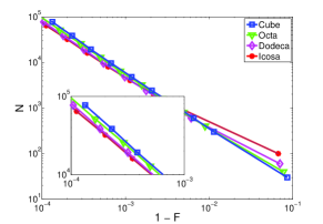
Simulation results for atomic qubit states are shown in Fig. 5(a). The tetrahedron is not plotted because for atomic measurements orthogonal outcomes are always measured simultaneously so, as noted above, the tetrahedron measurement does not arise without more experimental effort. Observe that, for sufficiently large $N$, increasing the order of the Platonic solid improves tomography performance. Recall that $N$ is the total number of systems measured so this result holds despite the fact that each outcome probability is estimated from a smaller number of measurements. The improvement of the icosahedron over the dodecahedron is only marginal but the difference in performance from the other measurements is statistically significant.

VIII.2 Two atomic qubit state results

The simulation results for two qubit atomic states are shown in Fig. 5(b). The performance is effectively the same for all the Platonic solids and experimentally one should choose the cube tensor measurement to minimize the time consumed by changes in measurement settings.

VIII.3 Single photonic qubit results

The single photonic qubit results using a single photon counter are shown in Fig. 5(c). In addition to the Platonic solid measurement sets, we have also included, the popular measurement sets proposed by James et al. in James et al. (2001). This set is labelled James4. The most striking aspect of these results is how poorly the James4 measurement set performs compared to the Platonic solids. It is a strong recommendation that experimentalists using this measurement set should switch to Platonic solid measurements. The performance of dual Platonic solids is similar (the cube and octagon, and the dodecahedron and the icosahedron), so we recommend using the cube or dodecahedron measurements.

(a) 1 atomic qubit	(c) 1 photonic qubit
(b) 2 atomic qubits	(d) 2 photonic qubits

Figure 6: Tomography simulation results with the prior induced by the quantum Chernoff bound. The number of copies is plotted against $1{-}\lambda_{av}$, where $\lambda_{av}$ is the average quantum Chernoff bound. Tomography for (a) a single atomic qubit, (b) two atomic qubits, (c) a single photonic qubit with a single-detector configuration, (d) two photonic qubits using single-detector configurations.

VIII.4 Two photonic qubit state results

The photonic two-qubit simulation results with single-detectors (one for each qubit subsystem) are shown in Fig. 5(d). In addition to the Platonic solid measurement sets, we have also included, the popular measurement sets proposed by James et al. in James et al. (2001) labelled James16, and the projective SicPOVM measurements.

Again the most striking result is how poorly the James16 measurement set performs compared to tensor products of Platonic solids. It is our strong recommendation that experimentalists using these settings change to a measurement consisting of tensor products of cube measurements or if measurement setting changes consume too much time, at least to tensors of the tetrahedral measurements.

We also observe that while the projective SicPOVM performed the best, its improvement was negligible over the cube tensors. There seems to be negligible advantage to going to Platonic solids any higher order than the cube.

IX Using the Quantum Chernoff bound as a figure of merit

As discussed in section II we find the use of the average quantum Chernoff bound to be the most physically appealing figure of merit. It is thus important to see if our conclusions hold when the quantum Chernoff bound is used instead of the fidelity.

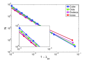
We repeated our tomography simulations using the average quantum Chernoff bound as the figure of merit, and the Chernoff bound prior over states. The results for one and two atomic qubits are shown in Figs. 6(a) and 6(b) respectively. The results for one and two photonic qubits with single-detector configurations are shown in Figs. 6(c) and 6(d) respectively.

In all cases the graphs are almost identical to those using a Bures prior and average fidelity as a figure of merit. It is clear that all of our conclusions from the average fidelity are correct, and hold also when using the quantum Chernoff figure of merit.

X Using the mean squared Hilbert-Schmidt distance as a figure of merit

While we have focussed on the average fidelity and the average Quantum Chernoff bound as our figures of merit for tomography schemes, there is one commonly used figure of merit that does behave quite differently and does affect our results — the mean squared Hilbert-Schmidt distance.

Roy and Scott Roy and Scott (2007) found Mutually Unbiased Bases (e.g. the cube measurement for a single qubit in our terminology) were an optimal measurement set for single qubit tomography using the mean squared Hilbert-Schmidt distance as a figure of merit. (They also neglect any effect of the positivity constraint on the density matrix, but our simulations bear out the hope that this is negligible.) These conclusions contrast to ours based on average fidelity which show that higher order Platonic solids perform better than cube measurements.

To explore this discrepancy we repeated the calculation of (15) (which also neglects the positivity constraints) replacing the fidelity with squared Hilbert-Schmidt distance to give a point squared Hilbert-Schmidt distance of:

$$\langle D_{hs}^{2}(r)\rangle\geq\frac{3}{2N}(3-r^{2})$$ (22)

where $r$ is the radius of the state on the Bloch sphere. This equation was derived in Rehacek et al. (2004) by other means and agrees with the results of Roy and Scott (2007). Observe the point squared Hilbert-Schmidt distance is independent of the angular parameters of the state on the Bloch sphere, unlike the point fidelity case which has an angular dependence, as shown in Eqn. (15).

We have repeated our numerical simulations using mean squared Hilbert-Schmidt distance as a figure of merit, a Bures prior and full maximum likelihood estimation. Our results show that for atomic qubits the Platonic solids all performed equivalently. Indeed our results were within statistical errors of the theoretical value obtained by integrating (22) over a Bures prior $D_{B}\geq 0.8438/N$. This suggests that the result of Roy and Scott (2007) that the cube measurement is optimal for mean squared Hilbert-Schmidt distance squared holds, even when the positivity constraint is included. We also note that for single-detector configurations our conclusions still hold, the James4 measurement set still performs badly and should be replaced by a cube measurement.

XI Discussion and conclusions

XI.1 Experimental Recommendations

The clear conclusion of this paper is that for single-detector photonic qubit tomography, experimentalists should immediately switch from the minimal four measurement set of James et al. (2001) to the overcomplete six measurement cube set, or at the very least switch to the tetrahedron measurement set if the number of measurement settings is an issue. Moving to the dual-detector configuration would further improve the results (subject to statistical fluctuation being the major source of error).

There is also a consistent trend towards better asymptotic performance for higher order Platonic solids for single qubit states. Experimentalists would have to judge whether there is a net gain after time to switch measurement settings is taken into account. We note that measurements on trapped ions are generally performing what we call the cube measurement set already.

We have found that this trend is maintained in two-qubit experiments with tensor product Platonic solid measurements performing very well even in comparison to entangled measurement sets. This strongly suggests that the use of these symmetrically arranged measurements will be advantageous for experiments on systems having larger numbers of qubits. In this case we note that the number of measurement settings grows very rapidly and the time to change between detector settings is likely to become an issue. In this regard the tetrahedron measurement should have much improved performance but requires no more measurements than the generalisations of James4 and James16.

We also note that while experiments in tomography usually report an uncertainty in the reconstruction based on a fixed number of measured systems, we are not aware of studies of how this uncertainty is reduced over time during the tomography. Such a study should contain information about the noise sources affecting the experiment. Specifically drifts in either the states or the measurement over time might be expected to lead to a saturation of the average fidelity with $N$. We have seen that when the experiment is limited by statistical noise then the quality of the tomography depends systematically on $N$ and on the choice of measurement. This could be tested experimentally and should give detailed information about the true errors in real experiments. In the case of optical experiments this simply requires rotating regularly among the different measurement settings and keeping track of the order in which counts arrive. State inversions can then be done at various time intervals and a graph of the number of qubits $N$ against point fidelity similar to our Fig. 3 could be straightforwardly obtained. One should, for example, be able to observe the general behaviour of a scaling like $1/\sqrt{N}$ at low numbers of copies transitioning to a scaling of $1/N$ at large numbers of copies. Likewise the improvement of the point fidelity with the choice of measurement could be checked. Comparison to detailed point fidelity simulations should aid characterization of experimental error sources.

XI.2 Future work

One could certainly consider measurements made from polyhedra other than the Platonic solids (for example the semi-regular polyhedra). However this paper has shown that the Platonic solids provide a good spread in the number of measurements and performance, and going to even higher order shapes appears to be of decreasing value. We thus consider exploring other shapes to be unfruitful with one likely exception. The SicPOVM was designed to be a spherical $t$ design with $t=2$. It is well known Hardin and Sloane (1996) that the cube and octagon are 3-designs while the dodecahedron and icosahedron are 5-designs. It is likely that this is the origin of the similarity in performance of the dual Platonic solids and $t$ is an indicator of the quality of tomography performance. This being the case it would be well worth investigating McLaren’s “improved Snub Cube” Hardin and Sloane (1996) which is a 24 point 7-design.

Appendix A Derivation of Pure State Cramér-Rao bounds for single qubit Tomography

Let $\eta=[\theta,\phi]^{T}$ be the state Bloch vector in spherical polar coordinates, and let $\hat{\eta}$ be the state estimate. The similarity between $\eta$ and $\hat{\eta}$ is given by the fidelity $f_{\eta}(\hat{\eta})=(1+r.\hat{r})/2$ where $r=[\cos(\phi)\sin(\theta),\sin(\phi)\sin(\theta),cos(\theta)]^{T}$ and similarly $\hat{r}=[\cos(\hat{\phi})\sin(\hat{\theta}),\sin(\hat{\phi})\sin(\hat{\theta}),cos(\hat{\theta})]^{T}$

Since we assume $\eta$ and $\hat{\eta}$ are close we expand the fidelity in a Taylor series to second order giving:

$$f_{\eta}(\hat{\eta})\approx f_{\eta}(\eta)+Df_{\eta}(\eta).(\hat{\eta}-\eta)+\frac{1}{2}(\hat{\eta}-\eta)H(\eta)(\hat{\eta}-\eta)^{T}$$ (23)

where $Df_{\eta}(\eta)_{i}=\frac{\partial f_{\eta}(\hat{\eta})}{\partial\eta_{i}}|_{\hat{\eta}=\eta}$ and $H(\eta)$ is the Hessian matrix defined by:

$$H(\eta)_{i,j}=\frac{\partial^{2}f_{\eta}(\hat{\eta})}{\partial\hat{\eta}_{i}\partial\hat{\eta}_{j}}\big{|}_{\hat{\eta}=\eta}.$$ (24)

Now $f_{\eta}(\eta)=1$ and $Df_{\eta}(\eta)=0$ so

$$f_{\eta}(\hat{\eta})\approx 1+\frac{1}{2}\sum_{i,j}\left.\frac{\partial^{2}f_{\eta}(\hat{\eta})}{\partial\eta_{i}\partial\eta_{j}}\right\rvert_{\hat{\eta}=\eta}(\hat{\eta}_{i}-\eta_{i})(\hat{\eta}_{j}-\eta_{j}).$$ (25)

During tomography, each of $N$ identical copies of the qubit state are each measured exactly once. Our measurement set consists of $l$ different measurement settings. So $\mathcal{N}=N/l$ measurements are performed with each measurement setting.

Each measurement setting is represented by Bloch vector $\vec{m_{i}}$, with outcomes $\chi_{i}{=}\pm{1}$. One set of measurements has $2^{l}$ possible outcomes represented by the string $\chi=\chi_{1}..\chi_{l}$. The probability of obtaining outcome $\chi$ is given by:

$$p_{\eta}(\chi)=\prod_{i}(1+\chi_{i}\vec{r}.\vec{m_{i}})/2.$$ (26)

The point fidelity obtained by averaging over the possible outcomes $\chi$ of the set of measurements is given by

$$F(\eta) = \sum_{\chi}p_{\eta}(\chi)f_{\eta}(\hat{\eta}(\chi))$$ (27)

$$\approx 1+\frac{1}{2}\mathrm{tr}[H(\eta)V(\eta)]$$ (28)

where $V(\eta)$ is the covariance matrix defined by:

$$V(\eta)=\sum_{\chi}p(\chi)(\hat{\eta}(\chi)-\eta)(\hat{\eta}(\chi)-\eta)^{T}.$$ (29)

The Cramér-Rao bound for unbiased estimators states:

$$V(\eta)\geq\frac{1}{\mathcal{N}I(\eta)}$$ (30)

where $I(\eta)$ is the Fisher Information matrix defined by:

$$I_{ij}(\eta)=\sum_{\chi}p_{\eta}(\chi)\frac{\partial\ln{p_{\eta}(\chi)}}{\partial\eta_{i}}\frac{\partial\ln{p_{\eta}(\chi)}}{\partial\eta_{j}}.$$ (31)

Noting that $H(\eta)$ is negative definite, the point fidelity bound is then given by:

$$F(\eta)\leq 1+\frac{1}{2\mathcal{N}}\mathrm{tr}[H(\eta)I^{-1}(\eta)].$$ (32)

Finally averaging over $\eta$ uniformly according to the Haar measure:

$$d\rho=\frac{\sin{\theta}}{4\pi}d\theta d\phi$$ (33)

gives average fidelity Cramér-Rao Bound.

Appendix B Eigenvalue distribution for the quantum Chernoff bound metric

In Audenaert et al. (2007) it was shown that the infinitesimal distance between states $\rho$ and $\rho{+}d\rho$ according to the Quantum Chernoff bound is:

$$ds^{2}=\frac{1}{2}\sum_{jk}\frac{|\mbox{$\langle j|$}d\rho\mbox{$|k\rangle$}|^{2}}{(\sqrt{\lambda_{j}}+\sqrt{\lambda_{k}})^{2}}$$ (34)

where $\rho=\sum_{j}\lambda_{j}\mbox{$|j\rangle$}\mbox{$\langle j|$}$ is the eigenvalue decomposition of $\rho$. We will follow the same procedure as Hall (1998) in his calculation of the Bures volume element to derive our quantum Chernoff bound eigenvalue distribution.

First decompose this into an infinitesimal shift in eigenvalues followed by an infinitesimal unitary rotation:

$$\rho+\delta\rho = (I+\delta U)(\rho+\delta\Lambda)(I+\delta U)^{\dagger}$$ (35)

$$= \rho+\delta\Lambda+[\delta U,\rho]$$ (36)

where we have ignored any terms which are a product of multiple infinitesimal quantities and defined $\mbox{$\langle j|$}\delta\Lambda\mbox{$|k\rangle$}=\delta_{jk}d\lambda_{j}$. In general we can rewrite the infinitesimal unitary operator as:

$$\delta U=\sum_{j\leq k}(dx_{jk}+idy_{jk})\mbox{$|j\rangle$}\mbox{$\langle k|$}+h.c.$$ (37)

Next we substitute Eq. 37 and Eq. 36 into Eq. 34 yielding

$$ds^{2} = \frac{1}{8}\sum_{j}\frac{(d\lambda_{j})^{2}}{\lambda_{j}}+\sum_{j<k}\frac{(\lambda_{k}-\lambda_{j})^{2}}{(\sqrt{\lambda_{j}}+\sqrt{\lambda_{k}})^{2}}(dx_{jk}^{2}+dy_{jk}^{2}).$$

We convert this into a differential volume element by multiplying together all the $ds_{i}$ formed by a shift in each parameter $\lambda_{i}$ assuming the shift in the other parameters is zero. Since the volume element will require normalization we combine any constant factors. The final differential volume element is given by:

$$dV=C^{\prime}\frac{d\lambda_{1}..d\lambda_{M}}{\sqrt{\lambda_{1}..\lambda_{M}}}\prod_{k<j}\frac{(\lambda_{k}-\lambda_{j})^{2}}{(\sqrt{\lambda_{j}}+\sqrt{\lambda_{k}})^{2}}dx_{jk}dy_{jk}$$ (38)

where $C^{\prime}$ is a normalisation constant.

Since the eigenvalue distribution is unitarily invariant we can concern ourselves with the marginal probability distribution over the eigenvalues of the density operators. That is:

$$p(\lambda_{1}..\lambda_{M})=\frac{C}{\sqrt{\lambda_{1}..\lambda_{M}}}\prod_{k<j}\frac{(\lambda_{k}-\lambda_{j})^{2}}{(\sqrt{\lambda_{j}}+\sqrt{\lambda_{k}})^{2}}$$ (39)

where the eigenvalues are also constrained to satisfy $\sum_{j=1}^{M}\lambda_{j}=1$ and $C$ is a normalisation constant. Next we examine the single qubit case.

B.1 Single Qubit Case

For the qubit case we have:

$$p(\lambda_{1}\lambda_{2})=\frac{C}{\sqrt{\lambda_{1}\lambda_{2}}}\frac{(\lambda_{1}-\lambda_{2})^{2}}{(\sqrt{\lambda_{1}}+\sqrt{\lambda_{2}})^{2}}$$ (40)

The eigenvalues for the qubit case are related to $r$ the radius on the Bloch sphere according to: $\lambda_{1}{=}(1{+}r)/2$ and $\lambda_{2}{=}(1{-}r)/2$. This yields

$$p(r)=\frac{C}{2}\frac{1-\sqrt{1-r^{2}}}{\sqrt{1-r^{2}}}$$ (41)

By requiring $\int_{0}^{1}p(r)dr=1$ we calculate $C{=}4/(\pi{-}2)$.

References

- Vogel and Risken (1989) K. Vogel and H. Risken, Phys. Rev. A 40, 2847 (1989).
- Leonhardt (1995) U. Leonhardt, Phys. Rev. Lett. 74, 4101 (1995).
- White et al. (1999) A. G. White, D. F. V. James, P. H. Eberhard, and P. G. Kwiat, Phys. Rev. Lett. 83, 3103 (1999).
- Langford et al. (2004) N. K. Langford, R. B. Dalton, M. D. Harvey, J. L. O’Brien, G. J. Pryde, A. Gilchrist, S. D. Bartlett, and A. G. White, Phys. Rev. Lett. 93, 053601 (2004).
- Haeffner et al. (2005) H. Haeffner, W. Haensel, C. F. Roos, J. Benhelm, D. C. al kar, M. Chwalla, T. Koerber, U. D. Rapol, M. Riebe, P. O. Schmidt, C. Becher, O. Guhne, W. Dur, R. Blatt, et al., Nature 438, 643 (2005).
- Reichle et al. (2006) R. Reichle, D. Leibfried, E. Knill, J. Britton, R. B. Blakestad, J. D. Jost, C. Langer, R. Ozeri, S. Seidelin, and D. J. Wineland, Nature 443, 838 (2006).
- Massar and Popescu (1995) S. Massar and S. Popescu, Phys. Rev. Lett. 74, 1259 (1995).
- Vidal et al. (1999) G. Vidal, J. I. Latorre, P. Pascual, and R. Tarrach, Phys. Rev. A 60, 126 (1999).
- Latorre et al. (1998) J. I. Latorre, P. Pascual, and R. Tarrach, Phys. Rev. Lett. 81, 1351 (1998).
- Holevo (1982) A. S. Holevo, Probabilistic and Statistical Aspects of Quantum Theory (North-Holland, Amsterdam, 1982).
- Derka et al. (1998) R. Derka, V. Buzek, and A. K. Ekert, Phys. Rev. Lett. 80, 1571 (1998).
- James et al. (2001) D. F. V. James, P. G. Kwiat, W. J. Munro, and A. G. White, Phys. Rev. A 64, 052312 (2001).
- Paris and Rehacek (2004) M. Paris and J. Rehacek, eds., Quantum State Estimation (Springer, 2004).
- Jones (1991) K. R. W. Jones, Ann. Phys. 207, 140 (1991).
- Bagan et al. (2005) E. Bagan, A. Monras, and R. Munoz-Tapia, Phys. Rev. A 71, 062318 (2005).
- Gill and Massar (2002) R. D. Gill and S. Massar, Phys. Rev. A 61, 042312 (2002).
- Bagan et al. (2006) E. Bagan, M. A. Ballester, R. D. Gill, R. Munoz-Tapia, and O. Romero-Isart, Phys. Rev. Lett. 97, 130501 (2006).
- Rehacek et al. (2004) J. Rehacek, B.-G. Englert, and D. Kaszlikowski, Phys. Rev. A 70, 052321 (2004).
- Roy and Scott (2007) A. Roy and A. J. Scott, Weighted complex projective 2-designs from bases: optimal state determination by orthogonal measurements (2007), quant-ph/0703025.
- Fuchs (1996) C. A. Fuchs, Distinguishability and accessible information in quantum theory (1996), quant-ph/9601020.
- Audenaert et al. (2007) K. M. R. Audenaert, J. Calsamiglia, L. Masanes, R. Munoz-Tapia, A. Acin, E. Bagan, and F. Verstraete, Phys. Rev. Lett. 98, 160501 (2007).
- Caves et al. (2002) C. M. Caves, C. A. Fuchs, and R. Schack, J. Math. Phys. 43, 4537 (2002).
- Blume-Kohout and Hayden (2006) R. Blume-Kohout and P. Hayden, Accurate quantum state estimation via ”keeping the experimentalist honest” (2006), quant-ph/0603116.
- Zyczkowski and Sommers (2001) K. Zyczkowski and H.-J. Sommers, J.PHYS.A 34, 7111 (2001).
- Hall (1998) M. J. W. Hall, Phys. Lett. A 242, 123 (1998).
- Munoz-Tapia (2007) R. Munoz-Tapia, Private communication (2007).
- Scott (2006) A. J. Scott, J. Phys. A 39, 13507 (2006).
- Renes et al. (2004) J. M. Renes, R. Blume-Kohout, A. J. Scott, and C. M. Caves, J. Math. Phys. 45, 2171 (2004).
- Hardin and Sloane (1996) R. H. Hardin and N. J. A. Sloane, Discrete Computational Geometry 15, 429 (1996).
- Decker et al. (2004) T. Decker, D. Janzing, and T. Beth, Int J. Quant. Inf. 2, 353 (2004).
- Englert et al. (2005) B.-G. Englert, T. K. Ming, G. C. Guan, and N. H. Khoon, Las. Phys. 15, 7 (2005).
- Bagan et al. (2002) E. Bagan, M. Baig, and R. Munoz-Tapia, Phys. Rev. Lett. 89, 277904 (2002).
- E. Bagan and Rodriguez (2004) R. M. E. Bagan, M. Baig and A. Rodriguez, Phys. Rev. A 69, 10304 (2004).
- Cirac et al. (2002) J. I. Cirac, L. M. Duan, and P. Zoller, Proceedings of the International School of Physics “Enrico Fermi” Course CXLVIII p. 263 (2002), quant-ph/0405030.
- (35) J. F. Sturn, Sedumi: A matlab toolbox for optimization over symmetric cones.