Critical fluctuations of time-dependent magnetization in a random-field Ising model

Abstract

Cooperative behaviors near the disorder-induced critical point in a random field Ising model are numerically investigated by analyzing time-dependent magnetization in ordering processes from a special initial condition. We find that the intensity of fluctuations of time-dependent magnetization, $\chi(t)$, attains a maximum value at a time $t=\tau$ in a normal phase and that $\chi(\tau)$ and $\tau$ exhibit divergences near the disorder-induced critical point. Furthermore, spin configurations around the time $\tau$ are characterized by a length scale, which also exhibits a divergence near the critical point. We estimate the critical exponents that characterize these power-law divergences by using a finite-size scaling method.

I Introduction

It has been known that earthquakes Sethna0 , acoustic emissions in a deformed complex material Grasso , and Barkhausen noise in random magnetsSethna1 ; Sethna2 ; Sethna3 ; Sabhapandit ; Durin ; Stanley exhibit distinctive power-law behaviors. All these systems possess some disorder and also they are driven by a slowly varying external field. As a simple model of such systems, a random field Ising model (RFIM) Young under a slowly varying magnetic field has been investigated in order to elucidate the essential mechanism of the power-law behaviors. By performing numerical experiments of the RFIM under a slowly increasing magnetic field, it was found that the size distribution of avalanches, each of which represents a spin flipping in a connected region, becomes a power-law function at the critical strength of the disorder Sethna1 . Then, the critical magnetic field at which the avalanche size becomes a system size is called disorder-induced critical point. Since this phenomenon occurs due to the existence of disorder, such power-law behaviors are called disorder-induced critical phenomena.

Despite the extensive studies for the critical phenomena, fluctuations of magnetization, which might be the most naive quantity characterizing the criticality, has never been investigated. Related to this issue, it has been known that the magnetization as a function of the magnetic field shows the almost discontinuous behavior at the disorder-induced critical point, although the precise determination of the transition type is still a controversySethna3 ; Vives2 ; Colaiori . From this observation and considering the knowledge of conventional critical phenomena, static fluctuations of magnetization hardly exhibit singular behaviors near the disorder-induced critical point. These raise a naive question whether the disorder-induced critical point can be characterized in terms of fluctuations of time-dependent magnetization.

In this paper, we present a positive answer to this question. Our key idea is to notice the recent extensive studies for critical fluctuations near an ergodicity breaking transition in glassy systems Onuki ; Bouchaud ; Garrahan ; Dauchot ; Biroli ; Miyazaki ; Sasa . Here, we review these studies briefly. As an example, let us consider cooperative behaviors near the transition point in colloidal suspensions. In this system, near the transition point, there exist long-range spatial correlations among movable particles during a time interval $\tau$, which is chosen as a typical relaxation time. When we introduce an appropriate quantity $Q({\bm{r}},t)$ that indicates the occurrence of large particle displacement at the position ${\bm{r}}$ during the time interval $t$, a discontinuous jump occurs in $Q({\bm{r}},t\to\infty)$ accompanied with critical fluctuations of $Q({\bm{r}},\tau)$ at the ergodicity breaking transition. It should be noted that $Q(r,t)$ characterizes the dynamical event intrinsic to glassy systems.

These results motivate us to study the cooperative behaviors near the disorder-induced critical point of the RFIM from the viewpoint of fluctuations of some dynamical events. In particular, we consider ordering processes of the magnetization from a special initial condition. We have numerically found that fluctuations of the time-dependent magnetization exhibit a critically divergent behavior near the disorder-induced critical point.

This paper is organized as follows. In Sec. II, we introduce the random-field Ising model and demonstrate its basic behaviors numerically. In Sec. III, we address the main result of our study. Concretely, we present new critical exponents that characterize the phenomena near the disorder-induced critical point. The final section is devoted to concluding remarks.

II Preliminaries

Let us consider a three-dimensional cubic lattice $\Lambda\equiv\{{\bm{i}}=(x,y,z)|1\leq x,y,z\leq L\}$. A spin variable $\sigma_{{\bm{i}}}\in\{-1,1\}$ is defined at each site ${\bm{i}}\in\Lambda$. We study the RFIM described by the Hamiltonian

$$H=-J\sum_{\left<{\bm{i}},{\bm{j}}\right>}\sigma_{{\bm{i}}}\sigma_{{\bm{j}}}-\sum_{{\bm{i}}\in\Lambda}(h_{{\bm{i}}}+h)\sigma_{{\bm{i}}},$$ (1)

where $\left<{\bm{i}},{\bm{j}}\right>$ represents a nearest-neighbor pair of sites, $h$ is a constant external field and the random field $h_{{\bm{i}}}$ obeys a Gaussian distribution

$$P(h_{{\bm{i}}})=\dfrac{1}{\sqrt{2\pi R^{2}}}\exp(-\frac{h_{{\bm{i}}}^{2}}{2R^{2}}).$$ (2)

The time evolution of the spin variables is described by the following rule. We first choose a site at random. If the spin flip on the site makes the system energy lower, the sign of the spin variable is changed; otherwise the spin flip is rejected. At the next step, we choose a site at random again, and repeat the above-mentioned procedure. Here, a unit time is given by $L^{3}$ steps, which is called a Monte Carlo step per site (MCS). This time evolution rule is similar to traditional avalanche dynamics such as the one used in Ref. Sethna3 , but our rule may be closer to standard Glauber dynamics. Indeed, it corresponds to the Metropolis method with the zero temperature. We should be careful to choose a time evolution rule particularly when we discuss finite temperature cases, but we do not enter a difficult question which time evolution rule is more physical.

Here, we review the disorder-induced critical phenomena in the RFIM. Let us consider the quasi static change of the external field from $h=-\infty$ to $h=\infty$. In this operation with a given $R$, $h_{\rm c}(R)$ is defined as the special value of $h$ (if it exists) at which a spin flipping in a region over the whole system first occurs. Then, $R_{\rm c}$ is defined as the maximum value below which $h_{\rm c}(R)$ exists. Their actual values were numerically determined as $(R_{\rm c},h_{\rm c}(R_{\rm c}))\simeq(2.16,1.44)$ Sethna3 , which is called disorder-induced critical point. It was reported that power-law behaviors of the size distribution of avalanches were observed in the quasi static change of the magnetic field when $R=R_{c}$. Such power-law behaviors are called the disorder-induced critical phenomena.

Figure 1: Ordering process of magnetization, $m(t)$. $L=40$ and $R=2.16$

In this paper, we study ordering processes of magnetization

$$\hat{m}(t) \equiv\frac{1}{N}\sum_{{\bm{i}}\in\Lambda}\sigma_{{\bm{i}}}(t)$$ (3)

from the initial condition $\hat{m}(0)=-1$ in which all the spins are downward. We also focus on the case $T=0$, except for a brief discussion in the final section. As preliminary calculations, we measure

$$m(t) \equiv\left<\hat{m}(t)\right>$$ (4)

for several values of $(R,h)$, where $\left<A\right>$ represents the average of a physical quantity $A$ with respect to the stochastic time evolution and quenched disorder. In the argument given below, we consider at least 20 samples of time evolution for each set of $\{h_{{\bm{i}}}\}$ and at least 20 samples of $\{h_{{\bm{i}}}\}$ for calculating average values.

Figure 2: $m(t_{\infty})$ as a function of $h$ for systems with three different sizes.

Typical samples of $m(t)$ for the case $R=2.16$ are displayed in Fig. 1. It is observed that the magnetization $m(t)$ quickly approaches the equilibrium value $m_{\rm eq}$, which is approximately 1, from -1 when $h$ is sufficiently large and that the ordering process becomes slower for the system with smaller $h$. Note that the equilibrium value $m_{\rm eq}$ is slightly less than $1$ because $h_{i}$ on some sites, whose values are largely negative, prevent the magnetization from approaching 1. Then, by decreasing $h$ further, we find that there is a value below which $m(t)$ does not reach the state with the equilibrium value $m_{\rm eq}$.

In order to quantify this transition, we consider the quantity $m(t_{\infty})$, where $t_{\infty}$ is chosen as 1000 MCSs in our numerical experiments. We confirmed that the results reported below did not depend on the choice of $t_{\infty}$ when $t_{\infty}\geq 1000$ MCSs. (The lowest value of $t_{\infty}$ depends on the system size.) On the basis of this, we define the frozen phase as the state with $m(t_{\infty})<m_{\rm eq}$. Since a discontinuous transition from $m_{\rm eq}$ to $m(t_{\infty})$ is expected to occur at a certain value of $h$ in the large size limit, we can replace the exact definition of the frozen phase with an operational one expressed as $m(t_{\infty})<1-\epsilon$, where $\epsilon=0.1$ for numerical simplicity. Indeed, as shown in Fig. 2, the transition becomes sharper when $L$ is larger. Therefore we expect that our operational definition provides an accurate determination of the phases in the large size limit. Presently, we fix $L=40$ and test whether the system exhibits a frozen phase for several values of $(R,h)$. The result is summarized in Fig. 3, which suggests the presence of a transition curve $h_{\rm b}(R,L,\epsilon)$ between the frozen and unfrozen phases. Note that the disorder-induced critical point $(R_{\rm c},h_{\rm c})$ reported in Ref. Sethna3 appears to be located on this curve. More precise correspondences with previous phase diagrams reported in Refs. Sethna2 ; Muller ; Vives will be discussed elsewhere.

Figure 3: Phase diagram. The circles represent frozen states. $L=40$.

III Result

Now, we focus on the behaviors near the disorder-induced critical point $(R_{\rm c},h_{\rm c})$. That is, by fixing $R$ as $R_{\rm c}$, we investigate the system with several values of $h$ near $h_{\rm c}$. Following our motivation, we are interested in studying fluctuations of $\hat{m}(t)$. It should be noted that our study is concerned with fluctuations of relaxation events. Although such types of fluctuations of dynamical events have been studied extensively in an ergodicity breaking transition in glassy systems, to our knowledge, there have been no such arguments on statistical properties near the disorder-induced critical point.

Since the simplest quantity characterizing the fluctuations of $\hat{m}(t)$ is given by

$$\chi(t) \equiv N\left[\left<\hat{m}(t)^{2}\right>-\left<\hat{m}(t)\right>^{2}\right],$$ (5)

we first demonstrate the graphs of $\chi(t)$ for a few values of $h$ in Fig. 4. It is observed that $\chi(t)$ has a peak at a time $\tau$ and that both $\chi_{\rm m}=\chi(\tau)$ and $\tau$ increase when $h$ approaches $h_{\rm c}(\simeq 1.44)$. Based on this observation, we next attempt to extract divergent behaviors of $\chi_{\rm m}$ and $\tau$ by using a finite-size scaling analysis.

Thus for the systems with $L=10$, $20$, and $40$, we measured $\tau(h,L)$ as a function of $(h-h_{\rm c})/h_{\rm c}$. As shown in the inset of Fig. 5, when we plot $\tau(h,L)L^{-a}$ as a function of $L^{1/\theta}(h-h_{\rm c})/h_{\rm c}$, these three graphs do not depend on $L$, where $a$ and $\theta$ are fitting parameters whose values ($\theta\simeq 0.7$ and $a\simeq 1.7$) are determined in such a manner that the three graphs are collapsed into a single curve as exactly as possible. Based on this result, we conjecture a scaling form

$$\tau(h,L) =L^{a}F_{\tau}\left(\left|\dfrac{h-h_{\rm c}}{h_{\rm c}}\right|L^{\frac{1}{\theta}}\right),$$ (6)

by using the scaling function $F_{\tau}$. Considering the asymptotic law $F_{\tau}(z)\simeq z^{-\zeta}$ (with $\zeta\simeq 1.3)$ in the regime $z\gg 1$, we expect the following critical behavior in the large size limit:

$$\tau\simeq(h-h_{\rm c})^{-\zeta}.$$ (7)

In a manner similar to that in the analysis of $\tau(h,L)$, we assume a form of the finite-size scaling as follows:

$$\chi_{m}(h,L) =L^{b}F_{\chi}\left(\left|\dfrac{h-h_{\rm c}}{h_{\rm c}}\right|L^{\frac{1}{\theta}}\right).$$ (8)

Indeed, from Fig. 5, we determine $b$ and the scaling function $F_{\chi}$, where $b\simeq 3.0$ and we find the asymptotic relation $F_{\chi}(z)\simeq z^{-\gamma}$ (with $\gamma\simeq 2.1$) in the regime $z\gg 1$. We thus obtain

$$\chi_{\rm m}\simeq(h-h_{\rm c})^{-\gamma}.$$ (9)

Figure 4: $\chi(t)$ for three values of $h$. $R=2.16$.

Figure 5: Finite-size scaling for $\chi_{m}(h,L)$ and $\tau(h,L)$ (inset). The three graphs for systems with different sizes are collapsed into a single curve. The statistical error bars are within the size of symbols. $h_{\rm c}=1.44$ and $R=2.16$.

Figure 6: $S({\bm{k}})/S({\bm{0}})$ as a function of $k\xi(h,L)$ Inset: Finite-size scaling for $\xi(h,L)$. Filled symbols represent those of the system for L=64 and the others for L=32. $R=2.16$.

These divergent behaviors observed near the disorder-induced critical point lead us to expect that some spins flip cooperatively around the time $\tau$. In order to describe the nature of the cooperative phenomena, we attempt to define a spatial correlation length that characterizes it, as carried out in studies on traditional critical phenomena. Here, it should be noted that the magnetization grows around the time $\tau$. In this paper, for numerical simplicity, we focus on the spin configurations at the time $t_{0}$ such that $\hat{m}(t_{0})=0$ for each sample because the magnetization is expected to grow at this time. We then consider the spatial pattern indicating whether the spin on each site has already flipped by the time $t_{0}$. Thus, we measure

$$\rho({\bm{j}}) =\delta(\sigma_{{\bm{j}}}(t_{0}),1),$$ (10)

where $\delta(m,n)$ represents Kronecker’s delta. Calculating its Fourier transform

$$\tilde{\rho}({\bm{k}}) =\sum_{{\bm{j}}\in\Lambda}\rho({\bm{j}})\exp(i{\bm{k}}\cdot{\bm{j}}),$$ (11)

we define the structure function

$$S({\bm{k}}) \equiv\frac{1}{N}\left<|\tilde{\rho}({\bm{k}})|^{2}\right>,$$ (12)

where we set ${\bm{k}}=(k,0,0)$ in the argument given below. For $S({\bm{k}})$ obtained for several values of $(h,L)$, we find that the fitting

$$S({\bm{k}})=\frac{S({\bm{0}})}{1+(\xi k)^{n}}$$ (13)

is obtained well with $n=3/2$, as shown in Fig. 6. This is called the Ornstein-Zernike form if $n=2$ Onuki . Then, $\xi$ represents the correlation length characterizing the spatial pattern $\rho({\bm{i}})$.

Now, in the same manner as those for $\tau$ and $\chi_{\rm m}$, we perform a finite-size scaling analysis assuming the form

$$\xi(h,L) =LF_{\xi}\left(\left|\dfrac{h-h_{\rm c}}{h_{\rm c}}\right|L^{\frac{1}{\theta}}\right).$$ (14)

The inset of Fig. 6 illustrates that this assumption is reasonable and that $F_{\xi}(z)$ obeys the asymptotic relation $F_{\xi}(z)\simeq z^{-\nu}$ for large $z$ ($\nu\simeq 0.7$). On the basis of this, we obtain the critical behavior of the dynamical correlation length:

$$\xi\simeq|h-h_{\rm c}|^{-\nu}.$$ (15)

Note that the obtained value $\nu\simeq 0.7$ is close to the value $\theta\simeq 0.7$, where $\theta$ is the exponent that characterizes the length scale appearing in the finite-size scaling method. This coincidence implies that the manner of the divergence for length scales is characterized by a single exponent. It should be noted that the exponents characterizing the length scale appearing in finite-size scaling analysis for statistical quantities related to avalanches were obtained in Refs. Dahmen ; Vives2 , where the values of the exponent are close to that of $\theta$ in our study. The relation among these results will be studied in the future.

One may be afraid that another time evolution rule provides a different result, in particular with regard to the exponent $\zeta$. Until now, we do not understand its dependency, but we conjecture that the value of $\nu$ is not so influenced by the choice of the time evolution rule, because of the consistency with the previous studies. These will be also studied in the future.

IV Concluding remarks

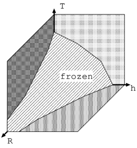
Figure 7: Schematic phase diagram in the (R,H,T) space.

We have presented the power-law divergences (7), (9), and (15) near the disorder-induced critical point in the RFIM. We have determined the exponents by using the finite-size scaling method as $\gamma\simeq 2.1$, $\zeta\simeq 1.3$ and $\nu\simeq 0.7$. These values are regarded as preliminary values and more precise values will be determined by using systems with considerably larger sizes. At present, the accuracy of values is not of primary interest, but the existence of divergent fluctuations of time-dependent magnetization is rather important. Indeed, based on our results, we conclude that the phenomena near the disorder-induced critical point can be captured from the viewpoint of fluctuations of dynamical events. In this sense, the phenomena under consideration have common features with cooperative behavior in glassy and jamming systems. It is an important future subject whether the values of critical exponents observed near the disorder-induced critical point are related to those in glassy and jamming systems.

Last, we introduce a few examples of studies motivated by this conclusion. The first example is the phase diagram in the $(R,H,T)$ space. Since the precise definition of the frozen phase appears to be complicated in the finite temperature case, we just plotted the region $m(t_{\infty})<0$ as a tentative frozen phase, using a Metropolis method. Figure 7 shows a schematic diagram of this phase. From this figure, one may recall the phase diagram of the jamming transition in granular systems (see Fig. 1 in Ref. Nagel or Fig. 4 in Ref Weitz ). We also expect that a similar type of phase diagram can be obtained when we employ other time evolution rules such as a heat bath method. Thus this resemblance motivates us to study the common aspects between granular systems and the present system.

The second example is related to a theoretical framework. In addition to extensive analysis on the power-law distribution of avalanches Sethna2 ; Sabhapandit ; Stanley , it was conjectured that the critical behaviors of avalanches in some spin models with disorder are related to metastable states Horbach ; Zimanyi ; Tarjus . It is interesting to investigate $\chi(t)$ in such systems. Furthermore, we are interested in conducting a theoretical analysis of our numerical results. Since $\chi(t)$ proposed in this paper has never been studied in the RFIM, such a theoretical analysis would shed light on a new aspect of the RFIM.

- (1) J. P. Sethna, K. A. Dahmen, and C. R. Myers, Nature 410, 242 (2001).
- (2) M. C. Miguel, A. Vespignani, S. Zapperi, J. Weiss, and J. R. Grasso, Nature 410, 667 (2001).
- (3) T. Nattermann, Spin Glasses and Random Fields, Series on Directions in Condensed Matter Physics, edited by A. P. Young (World Scientific, Singapore 1998) Vol. 12, pp. 277-298.
- (4) J. P. Sethna, K. A. Dahmen, S. Kartha, J. A. Krumhansl, B. W. Roberts, and J. D. Shore, Phys. Rev. Lett. 70, 3347 (1993).
- (5) K. A. Dahmen and J. P. Sethna, Phys. Rev. Lett. 71, 3222 (1993), Phys. Rev. B 53, 14872 (1996).
- (6) O. Perkovic, K. A. Dahmen, and J. P. Sethna, Phys. Rev. B 59, 6106 (1999).
- (7) S. Zapperi, P. Cizeau, G. Durin, and H. E. Stanley, Phys. Rev. B 58, 6353 (1998).
- (8) G. Durin and S. Zapperi, Phys. Rev. Lett 84, 4705 (2000).
- (9) S. Sabhapandit, D. Dhar, and P. Shukla, J. Stat. Phys. 98, 103 (2000).
- (10) F. J Perez-Reche and E. Vives, Phys. Rev. B 70, 214422 (2004).
- (11) F. Colaiori, M. J. Alava, G. Durin, A. Magni, and S. Zapperi, Phys. Rev. Lett. 92, 257203 (2004)
- (12) R. Yamamoto and A. Onuki, Phys. Rev. E 58, 3515 (1998).
- (13) L. Berthier, G. Biroli, J. P. Bouchaud, L. Cipelletti, D. E. Masri, D. L. Hote , F. Ladieu, and M. Pierno, Science 310, 1797 (2005).
- (14) O. Dauchot, G. Marty, and G. Biroli, Phys. Rev. Lett. 95, 265701 (2005).
- (15) D. Chandler, J. P. Garrahan, R. L. Jack, L. Maibaum , and A. C. Pan, Phys. Rev. E 74, 051501 (2006).
- (16) G. Biroli and J. P. Bouchaud, Europhys. Lett. 67, 21 (2004).
- (17) G. Biroli, J. P. Bouchaud, K. Miyazaki, and D. R. Reichman, Phys. Rev. Lett. 97, 195701 (2006).
- (18) M. Iwata and S. Sasa, Europhys. Lett. 77, 50008 (2007).
- (19) M. Muller and A. Silva, Phys. Rev. Lett. 96, 117202 (2006).
- (20) X. Illa, P. Shukla, and E. Vives, Phys. Rev. B 73, 092414 (2006).
- (21) J. H. Carpenter and K. A. Dahmen, Phys. Rev. B 67, 020412(R) (2003).
- (22) A. L. Liu and S. R. Nagel, Nature 396, 21 (1998).
- (23) V. Trappe, V. Prasad , L. Cipelletti, P. N. Segre, and D. A. Weitz, Nature 411, 772 (2001).
- (24) F. Pazmandi, G. Zarand, and G. T. Zimanyi, Phys. Rev. Lett. 83, 1034 (1999).
- (25) A. A. Pastor, V. Dobrosavljevic, and M. L. Horbach, Phys. Rev. B 66, 014413 (2002).
- (26) F. Detcheverry, M. L. Rosinberg, and G. Tarjus, Euro. Phys. J. B 44, 327 (2005).