Low Regularity local well-posedness for the 1+3 dimensional Dirac-Klein-Gordon system

Abstract.

We prove that the Cauchy problem for the Dirac-Klein-Gordon system of equations in 1+3 dimensions is locally well-posed in a range of Sobolev spaces for the Dirac spinor and the meson field. The result contains and extends the earlier known results for the same problem. Our proof relies on the null structure in the system, and bilinear spacetime estimates of Klainerman-Machedon type.

1. Introduction

We consider the Dirac-Klein-Gordon system (DKG) in three space dimensions,

$$\left\{\begin{aligned} \bigl{(}D_{t}+\alpha\cdot D_{x}\bigr{)}\psi=\phi\beta\psi,\quad\quad&(D_{t}=-i\partial_{t},\ D_{x}=-i\nabla)\\ \square\phi=-\left\langle\,\beta\psi,\psi\,\right\rangle,\quad\quad&(\square=-\partial_{t}^{2}+\Delta)\end{aligned}\right.$$ (1)

with initial data

$$\psi|_{t=0}=\psi_{0}\in H^{s},\qquad\phi|_{t=0}=\phi_{0}\in H^{r},\qquad\partial_{t}\phi|_{t=0}=\phi_{1}\in H^{r-1},$$ (2)

where $\psi(t,x)$ is the Dirac spinor, regarded as a column vector in $\mathbb{C}^{4}$, and $\phi(t,x)$ is the meson field which is real-valued; both the Dirac spinor and the meson field are defined for $t\in\mathbb{R},\ x\in\mathbb{R}^{3}$; $M,m\geq 0$ are constants; $\nabla=(\partial_{x_{1}},\partial_{x_{2}},\partial_{x_{3}})$; $\left\langle\,u,v\,\right\rangle:=\left\langle\,u,v\,\right\rangle_{\mathbb{C}^{4}}=v^{\dagger}u$ for column vectors $u,v\in\mathbb{C}^{4}$, where $v^{\dagger}$ is the complex conjugate transpose of $v$; $H^{s}=(1+\sqrt{-\Delta})^{-s}L^{2}(\mathbb{R}^{3})$ is the standard Sobolev space of order $s$. The Dirac matrices are given in $2\times 2$ block form by

$$\beta=\begin{pmatrix}I&0\\ 0&-I\end{pmatrix},\qquad\alpha^{j}=\begin{pmatrix}0&\sigma^{j}\\ \sigma^{j}&0\end{pmatrix},$$

where

$$\sigma^{1}=\begin{pmatrix}0&1\\ 1&0\end{pmatrix},\qquad\sigma^{2}=\begin{pmatrix}0&-i\\ i&0\end{pmatrix},\qquad\sigma^{3}=\begin{pmatrix}1&0\\ 0&-1\end{pmatrix}$$

are the Pauli matrices. The Dirac matrices $\alpha^{j},\beta$ satisfy

$$\beta^{\dagger}=\beta,\quad(\alpha^{j})^{\dagger}=\alpha^{j},\quad\beta^{2}=(\alpha^{j})^{2}=I,\quad\alpha^{j}\beta+\beta\alpha^{j}=0.$$ (3)

For the DKG system there are many conserved quantities which are not positive definite, such as the energy, see  [11]. However, there is a known positive conserved quantity, namely the charge, $\left\|\psi(t,.)\right\|_{L^{2}}=\text{const}$. To study questions of global regularity, a natural strategy is to study local (in time) well-posedness (LWP) for low regularity data, and then try to exploit the conserved quantities of the system. See, e.g., the global result of Chadam  [8] for 1+1 dimensional DKG system. The LWP results for DKG in 1+3 dimensions are summarized in Table 1

For DKG in 1+3 dimensions the scale invariant data is (see  [1])

$$(\psi_{0},\phi_{0},\phi_{1})\in L^{2}\times\dot{H}^{1/2}\times\dot{H}^{-1/2},$$

where $\dot{H}^{s}=(\sqrt{-\Delta})^{-s}L^{2}$. Heuristically, one cannot expect well-posedness below this regularity. This scaling also suggests that $r=1/2+s$ is the line where equation (1) is LWP. Concerning LWP of the DKG system in 1+3 dimensions, the best result to date is due to P. d’Ancona, D. Foschi and S. Selberg in  [1] for data

$$\psi_{0}\in H^{\varepsilon},\quad\phi_{0}\in H^{1/2+\varepsilon},\quad\phi_{1}\in H^{-1/2+\varepsilon},$$

where $\varepsilon>0$ is arbitrary. This result is arbitrarily close to the minimal regularity predicted by the scaling ($\varepsilon=0$). The key achievement in this result is that a null structure occurs not only in the Klein-Gordon part (in the nonlinearity $\left\langle\,\beta\psi,\psi\,\right\rangle$) which was known to be a null form (see  [1] for references)), but also in the Dirac part (in the nonlinearity $\phi\beta\psi$) of the system, which they discover using a duality argument. This requires first to diagonalize the system by using the eigenspace projections of the Dirac operator. The same authors used their result on the null structure in $\phi\beta\psi$ to prove LWP below the charge norm of the DKG system in 1+2 dimensions (see  [2]).

In the present paper we study the LWP of the DKG system in 1+3 dimensions. We prove that (1)–(2) is LWP for $(s,r)$ in the convex region shown in Figure 1, extending to the right, which contains the union of all the results shown in Table 1 as a proper subset. In our proof, we take advantage of the null structure in the nonlinearity $\phi\beta\psi$ found in  [1] besides the null structure in the nonlinearity $\left\langle\,\beta\psi,\psi\,\right\rangle$, and some bilinear spacetime estimates.

We now describe our main result.

Theorem 1.

Suppose $(s,r)\in\mathbb{R}^{2}$ belongs to the convex region described by (see Figure 1) the region

$$s>0,\qquad\max\left(\frac{1}{2}+\frac{s}{3},\frac{1}{3}+\frac{2s}{3},s\right)<r<\min\left(\frac{1}{2}+2s,1+s\right).$$

Then the DKG system (1) is LWP for data (2). Moreover, we can allow $r=1+s$ if $s>1/2$, and $r=s$ if $s>1$.

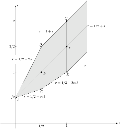
Figure 1. LWP holds in the interior of the shaded region, extending to the right. Moreover, we can allow the line $r=1+s$ for $s>1/2$, and the line $r=s$ for $s>1$. The line $r=1/2+s$ represents the regularity predicted by the scaling.

If $A,B,C,D$ are points in the $(s,r)$–plane, the symbol $AB$ represents a line from $A$ to $B$, $ABC$ represents a triangle and $ABCD$ a quadrilateral, all of them excluding the boundaries. We use the following notation for different regions in Figure 1:

$$R_{1}:=ACD\cup AD,$$ (4)

$$R_{2}:=ABD,$$

$$R_{3}:=D\cup F\cup CD\cup DF\cup FE\cup CDFE,$$

$$R_{4}:=G\cup BG\cup GF\cup BDGF,$$

$$R:=BD\cup\bigcup_{j=1}^{4}R_{j}.$$

Table 1. LWP exponents for (1), (2). That is, if the data $(\psi_{0},\phi_{0},\phi_{1})\in H^{s}\times H^{r}\times H^{r-1}$, then there exists a time $T>0$ and a solution of (1), $\bigl{(}\psi(t),\phi(t)\bigr{)}\in C\bigl{(}[0,T],H^{s}\bigr{)}\times C\bigl{(}[0,T],H^{r}\bigr{)}$ which depends continuously on the data. The solution is also unique in some subspace of $C\bigl{(}[0,T],H^{s}\bigl{)}\times C\bigl{(}[0,T],H^{r}\bigr{)}$. Here $\varepsilon>0$ is an arbitrary parameter.

	$s$	$r$
classical methods	$1+\varepsilon$	$3/2+\varepsilon$
Bachelot  [3], 1984	$1$	$3/2$
Strichartz estimate  [7, 15], 1993	$1/2+\varepsilon$	$1+\varepsilon$
Beals and Bezard  [4], 1996	$1$	$2$
Bournaveas  [7], 1999	$1/2$	$1$
Fang and Grillakis  [9], 2005	$(1/4,1/2]$	$1$
D’Ancona, Foschi and Selberg  [1], 2005	$\varepsilon$	$1/2+\varepsilon$

This paper is organized as follows. In the next section we fix some notation, state definitions and basic estimates. In addition, we shall rewrite the system (1) by splitting $\psi$ as the sum $P_{+}(D_{x})\psi+P_{-}(D_{x})\psi$, where $P_{\pm}(D_{x})$ are the projections onto the eigenspaces of the matrix $\alpha.D_{x}$. We also state the reduction of Theorem 1 to two $X^{s,b}$ bilinear estimates. In Section 3 we review the crucial null structure of the bilinear forms involved, and we discuss product estimates for wave-Sobolev spaces $H^{s,b}$. In Section 4 we interpolate between the product estimates from Section 3 to get a wider range of estimates. In Sections 5 and 6 we apply the estimates from Sections 3 and 4 to prove the bilinear estimates from Section 2. In Section 7 we prove that these bilinear estimates are optimal up to some endpoint cases, by constructing counterexamples.

For simplicity we set $M=m=0$ in the rest of the paper, but the discussion can easily be modified to handle the massive case as well.

2. Notation and preliminaries

In estimates, we use the symbols $\lesssim$, $\simeq$, $\gtrsim$ to denote relations $\leq$, $=$, $\geq$ up to a positive constant which may depend on $s$ and $r$. Also, if $K_{1}\lesssim K_{2}\lesssim K_{1}$ we will write $K_{1}\approx K_{2}$. If in the inequality $\lesssim$ the multiplicative constant is much smaller than 1 then we use the symbol $\ll$; similarly, if in $\gtrsim$ the constant is much greater than 1 then we use $\gg$. Throughout we use the notation $\langle\cdot\rangle=1+\left|\cdot\right|$. The characteristic function of a set $A$ is denoted by $\mathbb{1}_{A}$. For $a\in\mathbb{R}$, $a^{\pm}:=a\pm\epsilon$ for sufficiently small $\epsilon>0$. The Fourier transforms in space and space-time are defined by

$$\widehat{f}(\xi)=\int_{\mathbb{R}^{3}}e^{-ix\cdot\xi}f(x)\,dx,\qquad\widetilde{u}(\tau,\xi)=\int_{\mathbb{R}^{1+3}}e^{-i(t\tau+x\cdot\xi)}u(t,x)\,dt\,dx.$$

Then $\widetilde{D_{t}u}=\tau\widetilde{u}$, and $\widetilde{D_{x}u}=\xi\widetilde{u}$. If $\phi:\mathbb{R}^{3}\rightarrow\mathbb{C}$, we define the multiplier $\phi(D)$ by

$$\widehat{\phi(D)f}(\xi)=\phi(\xi)\widehat{f}(\xi).$$

Given $u(t,x)$, we denote by $\lfloor u\rfloor$ the function whose space-time Fourier transform is $\left|\widetilde{u}\right|$. If $X,Y,Z$ are normed function spaces, we use the notation $X\cdot Y\hookrightarrow Z$ to mean that

$$\left\|uv\right\|_{Z}\lesssim\left\|u\right\|_{X}\left\|v\right\|_{Y}.$$

In the study of non-linear wave equations it is standard that the following spaces of Bourgain-Klainerman-Machedon type are used. For $a,b\in\mathbb{R}$, define $X^{a,b}_{\pm}$, $H^{a,b}$ to be the completions of $\mathcal{S}(\mathbb{R}^{1+3})$ with respect to the norms

$$\left\|u\right\|_{X^{a,b}_{\pm}} =\bigl{\|}\langle\xi\rangle^{a}\langle\tau\pm\left|\xi\right|\rangle^{b}\widetilde{u}(\tau,\xi)\bigr{\|}_{L^{2}_{\tau,\xi}},$$

$$\left\|u\right\|_{H^{a,b}} =\bigl{\|}\langle\xi\rangle^{a}\langle\left|\tau\right|-\left|\xi\right|\rangle^{b}\widetilde{u}(\tau,\xi)\bigr{\|}_{L^{2}_{\tau,\xi}},$$

We also need the restrictions to a time slab $S_{T}=(0,T)\times\mathbb{R}^{3},$ since we study local in time solutions. The restriction $X_{\pm}^{a,b}(S_{T})$ is a Banach space with norm

$$\left\|u\right\|_{X_{\pm}^{a,b}(S_{T})}=\inf_{\tilde{u}_{\mid{S_{T}}}=u}\left\|\tilde{u}\right\|_{X_{\pm}^{a,b}}.$$

The restrictions $H^{a,b}(S_{T})$ is defined in the same way. We now collect some facts about these spaces which will be needed in the later sections. It is well known that the following interpolation property holds:

$$\left(H^{s_{0},\alpha_{0}},H^{s_{1},\alpha_{1}}\right)_{[\theta]}=H^{s,\alpha},$$ (5)

where $0\leq\theta\leq 1$, $s=(1-\theta)s_{0}+\theta s_{1}$, $\alpha=(1-\theta)\alpha_{0}+\theta\alpha_{1}$ and $(.,.)_{[\theta]}$ is the intermediate space with respect to the interpolation pair (.,.). It immediately follows from a general bilinear complex interpolation for Banach spaces (see for example  [6]) that if

$$H^{a_{0},\alpha_{0}}\cdot H^{b_{0},\beta_{0}} \hookrightarrow H^{-c_{0},-\gamma_{0}},$$

$$H^{a_{1},\alpha_{1}}\cdot H^{b_{1},\beta_{1}} \hookrightarrow H^{-c_{1},-\gamma_{1}},$$

then

$$H^{a,\alpha}\cdot H^{b,\beta}\hookrightarrow H^{-c,-\gamma},$$

where $0\leq\theta\leq 1$, $a=(1-\theta)a_{0}+\theta a_{1}$, $b=(1-\theta)b_{0}+\theta b_{1}$, $c=(1-\theta)c_{0}+\theta c_{1}$, $\alpha=(1-\theta)\alpha_{0}+\theta\alpha_{1}$, $\beta=(1-\theta)\beta_{0}+\theta\beta_{1}$ and $\gamma=(1-\theta)\gamma_{0}+\theta\gamma_{1}$.

We shall also need the fact that

$$X_{\pm}^{a,b}(S_{T})\hookrightarrow H^{a,b}(S_{T}) \hookrightarrow C\bigl{(}[0,T],H^{a}\bigr{)}\quad\text{provided}\ \ b>1/2,$$ (6)

$$X_{\pm}^{a,b}\hookrightarrow H^{a,b} \quad\text{for all }\ \ b\geq 0.$$ (7)

The embedding (6) is equivalent to the estimate

$$\left\|u(t)\right\|_{H^{a}}\leq C_{1}\left\|u\right\|_{H^{a,b}(S_{T})}\leq C_{2}\left\|u\right\|_{X_{\pm}^{a,b}(S_{T})},$$

for all $0\leq t\leq T$ and $C_{1},C_{2}\geq 1$. In the first inequality, $C_{1}$ will depend on $b$ (see  [1] for the proof), and the second inequality follows from the fact that $\langle\left|\tau\right|-\left|\xi\right|\rangle\leq\langle\tau\pm\left|\xi\right|\rangle$ (hence $C_{2}=1$), which also implies (7).

Following  [1], we diagonalize the system by defining the projections

$$P_{\pm}(\xi)=\frac{1}{2}\left(I\pm\hat{\xi}\cdot\alpha\right),$$

where $\hat{\xi}\equiv\frac{\xi}{\left|\xi\right|}$. Then the spinor field splits into $\psi=\psi_{+}+\psi_{-}$, where $\psi_{\pm}=P_{\pm}(D_{x})\psi$. Now applying $P_{\pm}(D_{x})$ to the Dirac equation in (1), and using the identities

$$\alpha\cdot D_{x} =\left|D_{x}\right|P_{+}(D_{x})-\left|D_{x}\right|P_{-}(D_{x}),$$ (8)

$$\quad P^{2}_{\pm}(D_{x})= P_{\pm}(D_{x})\quad\text{and}\quad P_{\pm}(D_{x})P_{\mp}(D_{x})=0,$$

we obtain

$$\left\{\begin{aligned} &\bigl{(}D_{t}+\left|D_{x}\right|\bigr{)}\psi_{+}=P_{+}(D_{x})(\phi\beta\psi),\\ &\bigl{(}D_{t}-\left|D_{x}\right|\bigr{)}\psi_{-}=P_{-}(D_{x})(\phi\beta\psi),\\ &\square\phi=-\left\langle\,\beta\psi,\psi\,\right\rangle,\end{aligned}\right.$$ (9)

which is the system we shall work with.

We iterate in the spaces

$$\psi_{+}\in X_{+}^{s,\sigma}(S_{T}),\quad\psi_{-}\in X_{-}^{s,\sigma}(S_{T}),\quad(\phi,\partial_{t}\phi)\in H^{r,\rho}\times H^{r-1,\rho}(S_{T}),$$

where

$$\frac{1}{2}<\sigma,\rho<1$$

will be chosen depending on $r,s$. By a standard argument (see  [1] for details) Theorem 1 then reduces to

$$\left\|P_{\pm}(D_{x})(\phi\beta P_{[\pm]}(D_{x})\psi)\right\|_{X^{s,\sigma-1+\varepsilon}_{\pm}} \lesssim\left\|\phi\right\|_{H^{r,\rho}}\left\|\psi\right\|_{X^{s,\sigma}_{[\pm]}},$$ (10)

$$\left\|\left\langle\,\beta P_{[\pm]}(D_{x})\psi,P_{\pm}(D_{x})\psi^{\prime}\,\right\rangle\right\|_{H^{r-1,\rho-1+\varepsilon}} \lesssim\left\|\psi\right\|_{X^{s,\sigma}_{[\pm]}}\left\|\psi^{\prime}\right\|_{X^{s,\sigma}_{\pm}},$$ (11)

for all $\phi,\psi,\psi^{\prime}\in\mathcal{S}(\mathbb{R}^{1+3})$, where $\pm$ and $[\pm]$ denote independent signs, and $\varepsilon>0$ is sufficiently small.

But in  [1], it was shown that (10) is equivalent, by duality, to an estimate similar to (11), namely

$$\left\|\left\langle\,\beta P_{[\pm]}(D_{x})\psi,P_{\pm}(D_{x})\psi^{\prime}\,\right\rangle\right\|_{H^{-r,-\rho}}\lesssim\left\|\psi\right\|_{{X_{[\pm]}^{s,\sigma}}}\left\|\psi^{\prime}\right\|_{X_{\pm}^{-s,1-\sigma-\varepsilon}}, \text{\ref{Bilinear-Dirac}}^{\prime}$$ ()

for all $\psi,\psi^{\prime}\in\mathbb{R}^{1+3}$. Note that in this formulation, the bilinear null form $\left\langle\,\beta P_{[\pm]}(D_{x})\psi,P_{\pm}(D_{x})\psi^{\prime}\,\right\rangle$,  appears again. Thus, Theorem 1 has been reduced to proving ($\text{\ref{Bilinear-Dirac}}^{\prime}$) and (11). We shall prove the following theorem, which implies Theorem 1.

Theorem 2.

Suppose

$$s>0,\qquad\max\left(\frac{1}{2}+\frac{s}{3},\frac{1}{3}+\frac{2s}{3},s\right)<r<\min\left(\frac{1}{2}+2s,1+s\right).$$ (12)

Then there exist $1/2<\rho,\sigma<1$ and $\varepsilon>0$ such that ($\text{\ref{Bilinear-Dirac}}^{\prime}$) and (11) hold simultaneously for all $\psi,\psi^{\prime}\in\mathcal{S}(\mathbb{R}^{1+3})$. Moreover, in addition to (12) we can allow $r=1+s$ if $s>1/2$, and $r=s$ if $s>1$. The parameters $\rho,\sigma$ can be chosen as follows:

$$\rho=1/2+\varepsilon,$$ (13)

$$\sigma=\begin{cases}1/2+s/3\quad&\text{if}\ \ (s,r)\in R_{1},\\ 1/2+s\quad&\text{if}\ \ (s,r)\in R_{2},\\ 5/6-s/3+\varepsilon\quad&\text{if}\ \ (s,r)\in R_{3},\\ 3/2-s+4\varepsilon\quad&\text{if}\ \ (s,r)\in R_{4},\\ 1-\varepsilon\quad&\text{if}\ \ (s,r)\in BD,\\ \text{any number in }(1/2,1)\quad&\text{otherwise},\end{cases}$$ (14)

with $\varepsilon>0$ sufficiently small depending on $s,r$ (see (4) to locate $(s,r)$ in the case of (14)).

3. Null structure and a product law for wave Sobolev spaces

Let us first discuss the null structure in $\left\langle\,\beta P_{[\pm]}(D_{x})\psi,P_{\pm}(D_{x})\psi^{\prime}\,\right\rangle$. The discussion here follows  [1]. Taking the spacetime Fourier transform on this bilinear form we get

$$\left[\left\langle\,\beta P_{[\pm]}(D_{x})\psi,P_{\pm}(D_{x})\psi^{\prime}\,\right\rangle\right]\,\,\widetilde{}\,\,(\tau,\xi)\\ =\int_{\mathbb{R}^{1+3}}\left\langle\,\beta P_{[\pm]}(\eta)\widetilde{\psi}(\lambda,\eta),P_{\pm}(\eta-\xi)\widetilde{\psi}^{\prime}(\lambda-\tau,\eta-\xi)\,\right\rangle\,d\lambda\,d\eta,$$

where we have $(\lambda-\tau,\eta-\xi)$ as an argument of $\tilde{\psi}^{\prime}$ instead of $(\tau-\lambda,\xi-\eta)$ because of the complex conjugation in the inner product. Since $P_{\pm}(\eta-\xi)^{\dagger}=P_{\pm}(\eta-\xi)$, and $P_{\pm}(\eta-\xi)\beta=\beta P_{\mp}(\eta-\xi)$, we obtain

$$\left\langle\,\beta P_{[\pm]}(\eta)\widetilde{\psi}(\lambda,\eta),P_{\pm}(\eta-\xi)\widetilde{\psi}^{\prime}(\lambda-\tau,\eta-\xi)\,\right\rangle$$

$$=\left\langle\,P_{\pm}(\eta-\xi)\beta P_{[\pm]}(\eta)\widetilde{\psi}(\lambda,\eta),\widetilde{\psi}^{\prime}(\lambda-\tau,\eta-\xi)\,\right\rangle$$

$$=\left\langle\,\beta P_{\mp}(\eta-\xi)P_{[\pm]}(\eta)\widetilde{\psi}(\lambda,\eta),\widetilde{\psi}^{\prime}(\lambda-\tau,\eta-\xi)\,\right\rangle.$$

The matrix $\beta P_{\mp}(\eta-\xi)P_{[\pm]}(\eta)$ is the symbol of the bilinear operator $(\psi,\psi^{\prime})\mapsto\left\langle\,\beta P_{[\pm]}(D_{x})\psi,P_{\pm}(D_{x})\psi^{\prime}\,\right\rangle$. By orthogonality, $P_{\mp}(\eta-\xi)P_{[\pm]}(\eta)$ vanishes when the vectors $[\pm]\eta$ and $\pm(\eta-\xi)$ line up in the same direction. The following lemma, proved in  [1], quantifies this cancellation. We shall use the notation $\measuredangle(\eta,\zeta)$ for the angle between vectors $\eta,\zeta\in\mathbb{R}^{3}$.

Lemma 1.

$\beta P_{\mp}(\eta-\xi)P_{[\pm]}(\eta)=O\left(\measuredangle([\pm]\eta,\pm(\eta-\xi))\right)$.

As a result of this lemma, we get

$$\left|\left\langle\,\beta P_{[\pm]}(D_{x})\psi,P_{\pm}(D_{x})\psi^{\prime}\,\right\rangle\,\,\widetilde{}\,\,(\tau,\xi)\right|\lesssim\int_{\mathbb{R}^{1+3}}\theta_{[\pm],\pm}\left|\widetilde{\psi}(\lambda,\eta)\right|\left|\widetilde{\psi}^{\prime}(\lambda-\tau,\eta-\xi)\right|\,d\lambda\,d\eta,$$ (15)

where $\theta_{[\pm],\pm}=\measuredangle\bigl{(}[\pm]\eta,\pm(\eta-\xi)\bigr{)}$.

The strategy for proving Theorem 2 is to make use of this null form estimate, (15), and reduce ($\text{\ref{Bilinear-Dirac}}^{\prime}$) and (11) to some well-known bilinear spacetime estimates of Klainerman-Machedon type for products of free waves. We now discuss some product laws for the wave Sobolev spaces $H^{a,\alpha}$ in the following theorems.

Theorem 3.

Let $d>1/2$. Then

$$H^{a,d}\cdot H^{b,d}\hookrightarrow L^{2},$$ (16)

provided that

$$a,b\geq 0,\quad\text{and}$$

$$a+b>1.$$

Proof.

By the same proof as in Corollary 3.3 in  [5], but using the dyadic estimates in Theorem 12.1 in  [10], we have, for any $\varepsilon>0$,

$$\left\|uv\right\|_{L^{2}(\mathbb{R}^{1+3)}}\lesssim\left\|u_{0}\right\|_{H^{1+\varepsilon}(\mathbb{R}^{3})}\left\|v_{0}\right\|_{L^{2}(\mathbb{R}^{3})}.$$

It follows by the transfer principle (see  [1], Lemma 4) that

$$H^{1+\varepsilon,d}\cdot H^{0,d}\hookrightarrow L^{2}.$$

Now, interpolation between

$$H^{1+\varepsilon,d}\cdot H^{0,d}\hookrightarrow L^{2},$$

$$H^{0,d}\cdot H^{1+\varepsilon,d}\hookrightarrow L^{2},$$

gives

$$H^{(1+\varepsilon)(1-\theta),d}\cdot H^{(1+\varepsilon)\theta,d}\hookrightarrow L^{2},$$

for $\theta\in[0,1]$. If there exists $\theta\in[0,1]$ such that $a\geq(1+\varepsilon)(1-\theta)$ ( $\Leftrightarrow\theta\geq 1-a/(1+\varepsilon))$ and $b\geq(1+\varepsilon)\theta$ ($\Leftrightarrow\theta\leq b/(1+\varepsilon)$), then we have

$$H^{a,d}\cdot H^{b,d}\hookrightarrow L^{2}.$$

If $a,b\geq 0$ and $a+b>1$, then such $\theta\in[0,1]$ exists, if we choose $\varepsilon>0$ small enough. This proves Theorem 3. ∎

Theorem 4.

[10, 13, 14]. Let $s_{1},s_{2},s_{3}\in\mathbb{R}$. For free waves $u(t)=e^{\pm it\left|D_{x}\right|}u_{0}$ and $v(t)=e^{[\pm]it\left|D_{x}\right|}u_{0}$ (where $\pm$ and $[\pm]$ are independent signs), we have the estimate

$$\left\|\left|D_{x}\right|^{-s_{3}}(uv)\right\|_{L^{2}(\mathbb{R}^{1+3)}}\lesssim\left\|u_{0}\right\|_{\dot{H}^{s_{1}}}\left\|v_{0}\right\|_{\dot{H}^{s_{2}}}$$ (17)

if and only if

$$s_{1}+s_{2}+s_{3}=1,\quad s_{1}+s_{2}>1/2,\quad s_{1},s_{2}<1.\\$$ (18)

As an application of Theorems 3 and 4 we have the following:

Theorem 5.

Suppose $s_{1},s_{2},s_{3}\in\mathbb{R}$  and  $d>1/2$. Then

$$H^{s_{1},d}\cdot H^{s_{2},d}\hookrightarrow H^{-s_{3},0}$$ (19)

provided $s_{1},s_{2},s_{3}$ satisfy

$$s_{1}+s_{2}+s_{3}=1,\quad s_{1}+s_{2}>1/2,$$ (20)

$$s_{1}+s_{3}\geq 0,\quad s_{2}+s_{3}\geq 0,$$

$$s_{1},s_{2}<1,$$

or

$$s_{1}+s_{2}+s_{3}>1,\quad s_{1}+s_{2}>1/2,$$ (21)

$$s_{1}+s_{3}\geq 0,\quad s_{2}+s_{3}\geq 0.$$

Proof.

First, let us prove (19) for $s_{1},s_{2},s_{3}\in\mathbb{R}$ satisfying (20). By Theorem 4 and the transfer principle (see  [1], Lemma 4), we obtain

$$H^{s_{1},d}\cdot H^{s_{2},d}\hookrightarrow H^{-s_{3},0}\quad\text{if}\ \ \begin{cases}&s_{1}+s_{2}+s_{3}=1,\\ &s_{1}+s_{2}>1/2,\\ &s_{1},s_{2},s_{3}\geq 0,\quad s_{1},s_{2}<1.\end{cases}$$ (22)

Note that in view of (20) at most one of $s_{1},s_{2},s_{3}$ can be $\leq 0$. But by the triangle inequality in Fourier space (i.e., Leibniz rule), we can always reduce the problem to the case $s_{1},s_{2},s_{3}\geq 0$. Indeed, if $s_{3}\leq 0$, then (19) reduces to

$$H^{s_{1}+s_{3},b}\cdot H^{s_{2},d}\hookrightarrow L^{2}\quad\text{and}\quad H^{s_{1},d}\cdot H^{s_{2}+s_{3},d}\hookrightarrow L^{2}.$$

In view of (22) these estimates hold for $s_{1},s_{2},s_{3}$ satisfying (20). If $s_{1}\leq 0$, then (19) reduces to

$$H^{0,d}\cdot H^{s_{1}+s_{2},d}\hookrightarrow H^{-s_{3},0}\quad\text{ and}\quad H^{0,d}\cdot H^{s_{2},d}\hookrightarrow H^{-(s_{1}+s_{3}),0},$$

and again by (22) these hold for $s_{1},s_{2},s_{3}$ satisfying (20). The case $s_{2}\leq 0$ is symmetrical to that of $s_{1}\leq 0$.

It remains to show (19) for $s_{1},s_{2},s_{3}$ satisfying (21). Write $s_{1}+s_{2}+s_{3}=1+\varepsilon$ where $\varepsilon>0$. We consider three cases: $s_{3}\leq 0$, $0<s_{3}<1/2$  and  $s_{3}\geq 1/2$.

Case 1: $s_{3}\leq 0$

In this case (using $s_{3}=1+\varepsilon-s_{1}-s_{2}$), (19) reduces to

$$\ H^{1+\varepsilon-s_{2},d}\cdot H^{s_{2},d}\hookrightarrow L^{2}\quad\text{and}\quad H^{s_{1},d}\cdot H^{1+\varepsilon-s_{1},d}\hookrightarrow L^{2},$$

which hold by Theorem 3 (since $s_{1},s_{2}\geq 0$, by (21) and the assumption $s_{3}\leq 0$).

Case 2: $0<s_{3}<1/2$

Here we consider three subcases: $s_{1}\leq 0$, $s_{2}\leq 0$ and $s_{1},s_{2}\geq 0$. By symmetry it suffices to consider $s_{1}\leq 0$ and $s_{1},s_{2}\geq 0$.

Assume $s_{1}\leq 0$; then (using $s_{3}=1+\varepsilon-s_{1}-s_{2}$) (19) reduces to

$$H^{0,d}\cdot H^{1+\varepsilon-s_{3},d}\hookrightarrow H^{-s_{3},0}$$ (23)

$$H^{0,d}\cdot H^{1+\varepsilon-s_{1}-s_{3},d}\hookrightarrow H^{-(s_{1}+s_{3}),0}.$$ (24)

Since (20) implies (19), we have

$$H^{0,d}\cdot H^{1/2+\varepsilon,d}\hookrightarrow H^{-(1/2-\varepsilon),0}\hookrightarrow H^{-1/2,0}.$$

Interpolating between this and

$$H^{0,d}\cdot H^{1+\varepsilon,d}\hookrightarrow L^{2},$$

with $\theta=2s_{3}$, gives (23) (note that $\theta\in(0,1)$ by the assumption on $s_{3}$). The same interpolation, but now with $\theta=2(s_{1}+s_{3})$ ($\theta\in[0,1]$ by the assumption on $s_{1}$ and $s_{3}$), gives (24).

Assume next $s_{1},s_{2}\geq 0$. Choose $0\leq s_{1}^{\prime}\leq s_{1}$, $0\leq s_{2}^{\prime}\leq s_{2}$ such that $s_{1}^{\prime},s_{2}^{\prime}<1$ and $s_{1}^{\prime}+s_{2}^{\prime}+s_{3}=1$. Indeed, we can choose such $s_{1}^{\prime}$ and $s_{2}^{\prime}$ as follows: If $s_{2}+s_{3}\leq 1$, take $s_{1}^{\prime}:=1-(s_{2}+s_{3})\in[0,1)$ and $s_{2}^{\prime}:=s_{2}\in[0,1)$. If $s_{2}+s_{3}>1$, take $s_{1}^{\prime}:=0$ and $s_{2}^{\prime}:=1-s_{3}\in(1/2,1).$ Then the problem reduces to

$$H^{s_{1}^{\prime},d}\cdot H^{s_{2}^{\prime},d}\hookrightarrow H^{-s_{3},0},$$

which holds since (20) implies (19).

Case 3: $s_{3}\geq 1/2$

Take $s_{3}^{\prime}=1/2-\delta$, where $\delta>0$ is chosen such that $s_{1}+s_{2}+s_{3}^{\prime}>1$ (this is possible due to the assumption $s_{1}+s_{2}>1/2$ in (19)). Then

$$H^{-s_{3}^{\prime},0}\hookrightarrow H^{-s_{3},0},$$

so the problem reduces to case 2 for $s_{1}$, $s_{2}$ and $s_{3}^{\prime}$. ∎

We also need the following product law for the Wave Sobolev spaces.

Theorem 6.

[16]. Let $t_{1},t_{2},t_{3}\in\mathbb{R}$. Then

$$H^{t_{1},d_{1}}\cdot H^{t_{2},d_{2}}\hookrightarrow H^{-t_{3},-d_{3}}$$ (25)

provided

$$t_{1}+t_{2}+t_{3}>3/2,$$ (26)

$$t_{1}+t_{2}\geq 0,\quad t_{2}+t_{3}\geq 0,\quad t_{1}+t_{3}\geq 0$$

$$d_{1}+d_{2}+d_{3}>1/2,$$

$$d_{1},d_{2},d_{3}\geq 0.$$

Moreover, we can allow $t_{1}+t_{2}+t_{3}=3/2$, provided $t_{j}\neq 3/2$ for $1\leq j\leq 3$. Similarly, we may take $d_{1}+d_{2}+d_{3}=1/2$, provided $d_{j}\neq 1/2$ for $1\leq j\leq 3$.

Proof.

In view of (26), at most one of $t_{1},t_{2},t_{3}$ can be negative. But by the same Leibniz rule as in the proof of Theorem 5 this can be reduced to the case $t_{1},t_{2},t_{3}\geq 0$, which was proved in [16, Proposition  10]. ∎

Theorem 7.

Let $\epsilon>0$. Then

$$H^{1/2+\epsilon,{1/2}^{+}}\cdot H^{\epsilon,{1/2}^{+}}\hookrightarrow H^{-1+\epsilon,1/2}.$$ (27)

Proof.

The embedding (27) is equivalent to the estimate

$$I\lesssim\left\|u\right\|_{L^{2}(\mathbb{R}^{1+3})}\left\|u\right\|_{L^{2}(\mathbb{R}^{1+3})},$$

where

$$I=\left\|\int_{\mathbb{R}^{1+3}}\frac{\langle\left|\tau\right|-\left|\xi\right|\rangle^{1/2}\widetilde{u}(\lambda,\eta)\widetilde{v}(\tau-\lambda,\xi-\eta)}{\langle\xi\rangle^{1-\epsilon}\langle\eta\rangle^{1/2+\epsilon}\langle\xi-\eta\rangle^{\epsilon}\langle\left|\lambda\right|-\left|\eta\right|\rangle^{{1/2}^{+}}\langle\left|\tau-\lambda\right|-\left|\xi-\eta\right|\rangle^{{1/2}^{+}}}d\lambda d\eta\right\|_{L^{2}_{(\tau,\xi)}}.$$

By the ’hyperbolic’ Leibniz rule (see  [12] lemma 3.2), we reduce this to three estimates

$$H^{1/2+\varepsilon,0}\cdot H^{\varepsilon,{1/2}^{+}}\hookrightarrow H^{-1+\varepsilon,0},$$

$$H^{1/2+\varepsilon,{1/2}^{+}}\cdot H^{\varepsilon,0}\hookrightarrow H^{-1+\varepsilon,0},$$

and (using also transfer principle to one free wave estimate)

$$\left\|\left|D_{x}\right|^{{-1+\epsilon}}D_{-}^{1/2}(uv)\right\|_{L^{2}}\lesssim\left\|\left|D_{x}\right|^{1/2+\epsilon/2}u_{0}\right\|_{L^{2}}\left\|\left|D_{x}\right|^{\epsilon/2}v_{0}\right\|_{L^{2}},$$

where $u=e^{\pm it\left|D_{x}\right|}u_{0}$ and $v=e^{\pm it\left|D_{x}\right|}v_{0}$, and the operator $D_{-}$ corresponds to the symbol $\left|\left|\tau\right|-\left|\xi\right|\right|$. The first two estimates hold by Theorem 6, and the last estimate holds by Theorem 1.1 in  [10]. ∎

4. Interpolation results

By bilinear interpolation between special cases of Theorems 5 and 6, and at one point Theorem 7, we obtain a series of estimates which will be useful in the proof of Theorem 2. For $a,b,c,\alpha,\beta,\gamma\in\mathbb{R}$, and $\epsilon>0$ sufficiently small, we obtain the following estimates (the proof is given below):

$$H^{a,\alpha}\cdot H^{0,{1/2}^{+}}\hookrightarrow H^{-c,0}\quad\text{if}\quad\begin{cases}&a,c,\alpha\geq 0,\\ &3\min(a/2,\alpha)+c>3/2.\\ \end{cases}$$ (28)

$$H^{a,\alpha}\cdot H^{0,{1/2}^{+}}\hookrightarrow H^{-c,0}\quad\text{if}\quad\begin{cases}&a,\alpha\geq 0,\ c\geq 1/2,\\ &\min(a,\alpha)+c/2>3/4.\\ \end{cases}$$ (29)

$$H^{a,\alpha}\cdot H^{0,\beta}\hookrightarrow H^{0,-\gamma}\quad\text{if}\quad\begin{cases}\ \ &a>1,\ \alpha>0,\ \beta,\gamma\geq 0,\\ &a+\min(\alpha,\beta)>3/2,\\ &\gamma+\min(\alpha,\beta)>1/2.\end{cases}$$ (30)

$$H^{a,{1/2}^{+}}\cdot H^{b,\beta}\hookrightarrow H^{-c,0}\quad\text{if}\quad\begin{cases}\ &c,\beta\geq 0,\ a,b>0,\\ &a+b=1,\\ &c+\beta>1/2.\end{cases}$$ (31)

$$H^{1,{1/2}^{+}}\cdot H^{0,\beta}\hookrightarrow H^{-c,0}\quad\text{if}\quad\begin{cases}&\beta\geq 0,\ c>0,\\ &c+\beta>1/2.\end{cases}$$ (32)

$$H^{a,\alpha}\cdot H^{b,{1/2}^{+}}\hookrightarrow H^{-c,0}\quad\text{if}\quad\begin{cases}&a,b,\alpha\geq 0,\ c\geq 1/2,\\ &\min(a,\alpha)+2b/3>1/2,\\ &\min(a,\alpha)+2c>3/2.\end{cases}$$ (33)

$$H^{a,{1/2}^{+}}\cdot H^{b,\beta}\hookrightarrow L^{2}\quad\text{if}\quad\begin{cases}&b,\beta\geq 0,\ a\geq 1/2,\\ &a+2\min(b,\beta)>3/2.\end{cases}$$ (34)

$$H^{a,{1/2}^{+}}\cdot H^{1/2,\beta}\hookrightarrow L^{2}\quad\text{if}\quad\begin{cases}&\beta\geq 0,\ a\geq 1/2,\\ &a+\beta>1.\end{cases}$$ (35)

$$H^{a,{1/2}^{+}}\cdot H^{\epsilon,\beta}\hookrightarrow H^{-1+\epsilon,-\gamma}\quad\text{if}\quad\begin{cases}&a,\beta\geq 0,\ \gamma\geq-1/2,\\ &\min(a,\beta)+\gamma/2>1/4.\end{cases}$$ (36)

$$H^{1/2,{1/2}^{+}}\cdot H^{0,\beta}\hookrightarrow H^{-c,0}\quad\text{if}\quad\begin{cases}&\beta\geq 0,\ c>1/2,\\ &c+\beta>1.\end{cases}$$ (37)

Proof of (28)–(37).

The parameter $\varepsilon>0$ is assumed to be sufficiently small.

To prove (28) we interpolate between

$$H^{1+\varepsilon,1/2+\varepsilon}\cdot H^{0,{1/2}^{+}} \hookrightarrow L^{2},$$

$$L^{2}\cdot H^{0,{1/2}^{+}} \hookrightarrow H^{-(3/2+\varepsilon),0}.$$

This gives

$$H^{(1+\varepsilon)(1-\theta),(1/2+\varepsilon)(1-\theta)}\cdot H^{0,{1/2}^{+}}\hookrightarrow H^{-(3/2+\varepsilon)\theta,0}$$

for $\theta\in[0,1]$. Now, if there exists $\theta\in[0,1]$ such that $a\geq(1+\varepsilon)(1-\theta)$  $\left(\Leftrightarrow\theta\geq 1-a/(1+\varepsilon)\right)$,  $\alpha\geq(1/2+\varepsilon)(1-\theta)$  $\left(\Leftrightarrow\theta\geq 1-2\alpha/(1+2\varepsilon)\right)$ and $c\geq(3/2+\varepsilon)\theta$  $\left(\Leftrightarrow\theta\leq 2c/(3+2\varepsilon)\right)$, then we have $H^{a,\alpha}\cdot H^{0,{1/2}^{+}}\hookrightarrow H^{-c,0}.$ But such a $\theta\in[0,1]$ exists if $a,\alpha,c\geq 0$, $3a+2c\geq 3+5\varepsilon-2\varepsilon(a+c)+2\varepsilon^{2}$ and $2c+6\alpha\geq 3+8\varepsilon-2\varepsilon(c+\alpha)+4\varepsilon^{2}$. Since $\varepsilon>0$ is very small, it is enough to have $a,\alpha,c\geq 0$, $3a+2c>3$ and $2c+6\alpha>3$. This proves (28). Interpolation between

$$H^{1/2+\varepsilon,1/2+\varepsilon}\cdot H^{0,{1/2}^{+}} \hookrightarrow H^{-(1/2+\varepsilon),0},$$

$$L^{2}\cdot H^{0,{1/2}^{+}} \hookrightarrow H^{-(3/2+\varepsilon),0},$$

with a similar argument as above, proves (29).

To prove (30), we interpolate between

$$H^{1+\varepsilon,1/2+\varepsilon}\cdot H^{0,1/2+\varepsilon} \hookrightarrow L^{2},$$

$$H^{3/2+\varepsilon,\varepsilon}\cdot L^{2} \hookrightarrow H^{0,-(1/2-\varepsilon)}.$$

This gives

$$H^{(1+\varepsilon)(1-\theta)+(3/2+\varepsilon)\theta,(1/2+\varepsilon)(1-\theta)+\varepsilon\theta}\cdot H^{0,(1/2+\varepsilon)(1-\theta)}\hookrightarrow H^{0,-(1/2-\varepsilon)\theta},$$

for $\theta\in[0,1]$. If there exists $\theta\in[0,1]$ such that $a\geq(1+\varepsilon)(1-\theta)+(3/2+\varepsilon)\theta$, $\alpha\geq(1/2+\varepsilon)(1-\theta)+\varepsilon\theta$, $\beta\geq(1/2+\varepsilon)(1-\theta)$  and $\gamma\geq(1/2-\varepsilon)\theta$ , then we have

$$H^{a,\alpha}\cdot H^{0,\beta}\hookrightarrow H^{0,-\gamma}.$$

By a similar argument as in the proof of (28), such a $\theta\in[0,1]$ exists if $a>1$, $\alpha>0$, $\beta,\gamma\geq 0$, $a+\alpha>3/2$, $a+\beta>3/2$, $\alpha+\gamma>1/2$ and $\beta+\gamma>1/2$. This proves (30).

To prove (31), we interpolate between

$$H^{a,{1/2}^{+}}\cdot H^{b,1/2+\varepsilon} \hookrightarrow L^{2},$$

$$H^{a,{1/2}^{+}}\cdot H^{b,0} \hookrightarrow H^{-1/2,0},$$

which both hold true if $a+b=1$, $a,b>0$, by Theorems 5 and 6, respectively. This gives

$$H^{a,{1/2}^{+}}\cdot H^{b,(1/2+\varepsilon)(1-\theta)}\hookrightarrow H^{-\theta/2,0}$$

for $\theta\in[0,1]$. If there exists $\theta\in[0,1]$ such that $\beta\geq(1/2+\varepsilon)(1-\theta)$ and $c\geq\theta/2$, then we have

$$H^{a,{1/2}^{+}}\cdot H^{b,\beta}\hookrightarrow H^{-c,0},$$

for $a+b=1$, $a,b>0$. By a similar argument as before such a $\theta\in[0,1]$ exists if $\beta,c\geq 0$ and $c+\beta>1/2$.

For (32)–(37), similar arguments as in the proof of (28) are used, so we only give the interpolation pairs, which give the desired estimate when interpolated.

For (32), we use

$$H^{1,{1/2}^{+}}\cdot H^{0,1/2+\varepsilon} \hookrightarrow H^{-\varepsilon,0},$$

$$H^{1,{1/2}^{+}}\cdot L^{2} \hookrightarrow H^{-1/2,0}.$$

For (33), we interpolate between

$$H^{1/2+\varepsilon,1/2+\varepsilon}\cdot H^{0,{1/2}^{+}} \hookrightarrow H^{-(1/2-\varepsilon),0},$$

$$L^{2}\cdot H^{3/4,{1/2}^{+}} \hookrightarrow H^{-3/4,0}.$$

For (34), we interpolate between

$$H^{1/2,{1/2}^{+}}\cdot H^{1/2,1/2+\varepsilon} \hookrightarrow L^{2},$$

$$H^{3/2+\varepsilon,{1/2}^{+}}\cdot L^{2} \hookrightarrow L^{2}.$$

For (35), we interpolate between

$$H^{1/2,{1/2}^{+}}\cdot H^{1/2,1/2+\varepsilon} \hookrightarrow L^{2},$$

$$H^{1,{1/2}^{+}}\cdot H^{1/2,0} \hookrightarrow L^{2}.$$

For (36), we interpolate between

$$H^{0,{1/2}^{+}}\cdot H^{\varepsilon,0} \hookrightarrow H^{-(1-\varepsilon),-(1/2+\varepsilon)},$$

$$H^{1/2+\varepsilon,{1/2}^{+}}\cdot H^{\varepsilon,1/2+\varepsilon} \hookrightarrow H^{-(1-\varepsilon),1/2},$$

where the second embedding holds by Theorem 7.

For (37), we interpolate between

$$H^{1/2,{1/2}^{+}}\cdot H^{0,1/2+\varepsilon} \hookrightarrow H^{-(1/2+\varepsilon),0},$$

$$H^{1/2,{1/2}^{+}}\cdot L^{2} \hookrightarrow H^{-1,0},$$

where the first embedding does not directly follow from Theorems 5 and 6, but from interpolation between

$$H^{1/2+\varepsilon,{1/2}^{+}}\cdot H^{0,1/2+\varepsilon} \hookrightarrow H^{-(1/2-\varepsilon),0},$$

$$H^{0,{1/2}^{+}}\cdot H^{0,1/2+\varepsilon} \hookrightarrow H^{-(3/2+\varepsilon),0},$$

which gives

$$H^{(1/2+\varepsilon)(1-\theta),{1/2}^{+}}\cdot H^{0,1/2+\varepsilon}\hookrightarrow H^{-(1/2-\varepsilon)(1-\theta)-(3/2+\varepsilon)\theta,0}$$

for $\theta\in[0,1]$. Choosing $\theta=\frac{2\varepsilon}{1+2\varepsilon}$ gives the desired estimate.

∎

In the following two sections, we shall present the proof of the bilinear estimates ($\text{\ref{Bilinear-Dirac}}^{\prime}$) and (11) for all $\psi,\psi^{\prime}\in\mathcal{S}(\mathbb{R}^{1+3})$ provided $(r,s)$, $\rho$ and $\sigma$ are as in (12), (13) and (14) respectively. These will imply Theorem 2. First we prove (11), and then ($\text{\ref{Bilinear-Dirac}}^{\prime}$). Note that using (7) we can reduce $X^{s,b}$ type estimates to $H^{s,b}$ type estimates, which we shall do in the following two sections.

5. Proof of (11)

Without loss of generality we take $[\pm]=+$. Assume $\psi,\psi^{\prime}\in\mathcal{S}(\mathbb{R}^{1+3})$ . Using (15), we can reduce (11) (write $\rho=1/2+\varepsilon$, as in (13)) to

$$I^{\pm}\lesssim\left\|\psi\right\|_{{X_{+}^{s,\sigma}}}\left\|\psi^{\prime}\right\|_{X_{\pm}^{s,\sigma}},$$

where

$$I^{\pm}=\left\|\int_{\mathbb{R}^{1+3}}\frac{\theta_{\pm}}{\langle\xi\rangle^{1-r}\langle\left|\tau\right|-\left|\xi\right|\rangle^{1/2-2\varepsilon}}\left|\widetilde{\psi}(\lambda,\eta)\right|\left|\widetilde{\psi}^{\prime}(\lambda-\tau,\eta-\xi)\right|\,d\lambda\,d\eta\right\|_{L^{2}_{\tau,\xi}},$$

and

$$\theta_{\pm}=\measuredangle\bigl{(}\eta,\pm(\eta-\xi)\bigr{)}.$$

The low frequency case, where $\min(|\eta|,|\eta-\xi|)\leq 1$ in $I^{\pm}$, follows from a similar argument as in  [2], and hence we do not consider this question here. From now on we assume that in $I^{\pm}$,

$$|\eta|,|\eta-\xi|\geq 1.$$ (38)

We shall use the following notation in order to make expressions manageable:

$$F(\lambda,\eta)=\langle\eta\rangle^{s}\langle\lambda+|\eta|\rangle^{\sigma}\left|\widetilde{\psi}(\lambda,\eta)\right|,\qquad G_{\pm}(\lambda,\eta)=\langle\eta\rangle^{s}\langle\lambda\pm|\eta|\rangle^{\sigma}\left|\widetilde{\psi}^{\prime}(\lambda,\eta)\right|,$$

$$\Gamma=\left|\tau\right|-\left|\xi\right|,\qquad\Theta=\lambda+|\eta|,\qquad\Sigma_{\pm}=\lambda-\tau\pm|\eta-\xi|,$$

$$\kappa_{+}=\left|\xi\right|-\bigl{|}|\eta|-|\eta-\xi|\bigr{|},\qquad\kappa_{-}=|\eta|+|\eta-\xi|-\left|\xi\right|.$$

We shall need the estimates (see  [1]):

$$\theta_{+}^{2}\sim\frac{\left|\xi\right|\kappa_{+}}{|\eta||\eta-\xi|},\qquad\theta_{-}^{2}\sim\frac{(|\eta|+|\eta-\xi|)\kappa_{-}}{|\eta||\eta-\xi|}\sim\frac{\kappa_{-}}{\min(|\eta|,|\eta-\xi|)}.$$ (39)

$$\kappa_{\pm} \leq 2\min(|\eta|,|\eta-\xi|),$$ (40)

$$\kappa_{\pm} \leq\left|\Gamma\right|+\left|\Theta\right|+\left|\Sigma_{\pm}\right|.$$ (41)

5.1. Estimate for $I^{+}$

By (39), and using (38)

$$I^{+}\lesssim\left\|\int_{\mathbb{R}^{1+3}}\frac{\kappa_{+}^{1/2}F(\lambda,\eta)G_{+}(\lambda-\tau,\eta-\xi)}{\langle\xi\rangle^{1/2-r}\langle\eta\rangle^{1/2+s}\langle\eta-\xi\rangle^{1/2+s}\langle\Gamma\rangle^{1/2-2\varepsilon}\langle\Theta\rangle^{\sigma}\langle\Sigma_{+}\rangle^{\sigma}}\,d\lambda\,d\eta\right\|_{L^{2}_{\tau,\xi}}.$$

By (40) and (41)

$$\kappa_{+}^{1/2}\lesssim\left|\Gamma\right|^{1/2-2\varepsilon}\min(|\eta|,|\eta-\xi|)^{2\varepsilon}+\left|\Theta\right|^{1/2}+\left|\Sigma_{+}\right|^{1/2}.$$

Moreover, by symmetry we may assume $|\eta|\geq|\eta-\xi|$ in $I^{+}$. By (12), $r>1/2$, so we have by the triangle inequality

$$\langle\xi\rangle^{r-1/2}\lesssim\langle\eta\rangle^{r-1/2}+\langle\eta-\xi\rangle^{r-1/2}\lesssim\langle\eta\rangle^{r-1/2}.$$ (42)

Hence the estimate reduces to

$$I_{j}^{+}\lesssim\left\|F\right\|_{L^{2}}\left\|G_{+}\right\|_{L^{2}},\ \ j=1,2,3,$$

where

$$I^{+}_{1} =\left\|\int_{\mathbb{R}^{1+3}}\frac{F(\lambda,\eta)G_{+}(\lambda-\tau,\eta-\xi)}{\langle\eta\rangle^{1+s-r}\langle\eta-\xi\rangle^{1/2+s-2\varepsilon}\langle\Theta\rangle^{\sigma}\langle\Sigma_{+}\rangle^{\sigma}}\,d\lambda\,d\eta\right\|_{L^{2}_{\tau,\xi}},$$

$$I^{+}_{2} =\left\|\int_{\mathbb{R}^{1+3}}\frac{F(\lambda,\eta)G_{+}(\lambda-\tau,\eta-\xi)}{\langle\eta\rangle^{1+s-r}\langle\eta-\xi\rangle^{1/2+s}\langle\Gamma\rangle^{1/2-2\varepsilon}\langle\Theta\rangle^{\sigma-1/2}\langle\Sigma_{+}\rangle^{\sigma}}\,d\lambda\,d\eta\right\|_{L^{2}_{\tau,\xi}},$$

$$I^{+}_{3} =\left\|\int_{\mathbb{R}^{1+3}}\frac{F(\lambda,\eta)G_{+}(\lambda-\tau,\eta-\xi)}{\langle\eta\rangle^{1+s-r}\langle\eta-\xi\rangle^{1/2+s}\langle\Gamma\rangle^{1/2-2\varepsilon}\langle\Theta\rangle^{\sigma}\langle\Sigma_{+}\rangle^{\sigma-1/2}}\,d\lambda\,d\eta\right\|_{L^{2}_{\tau,\xi}}.$$

5.1.1. Estimate for $I^{+}_{1}$

The problem reduces to

$$H^{1+s-r,\sigma}\cdot H^{s+1/2-2\varepsilon,\sigma}\hookrightarrow L^{2},$$

which holds by Theorem 5 for all $1/2<\sigma<1$ provided the conditions

$$s>-1/2\quad\ r<1/2+2s\quad\text{and}\quad r\leq 1+s$$

are satisfied, which they are by (12), and provided also that $\varepsilon>0$ is sufficiently small, which is tacitly assumed in the following discussion.

5.1.2. Estimate for $I^{+}_{2}$

We assume that $\left|\Gamma\right|\lesssim\min(\left|\eta\right|,\left|\eta-\xi\right|)=\left|\eta-\xi\right|$, since otherwise $I^{+}$ reduces to $I^{+}_{1}$ in view of (40). Giving up the weight $\langle\Theta\rangle^{-\sigma+1/2}$ in the integral, we get

$$I^{+}_{2}\lesssim\left\|\int_{\mathbb{R}^{1+3}}\frac{F(\lambda,\eta)G_{+}(\lambda-\tau,\eta-\xi)}{\langle\eta\rangle^{1+s-r}\langle\eta-\xi\rangle^{1/2+s-3\varepsilon}\langle\Sigma_{+}\rangle^{\sigma}\langle\Gamma\rangle^{1/2+\varepsilon}}\,d\lambda\,d\eta\right\|_{L^{2}_{\tau,\xi}}.$$

Then the problem reduces to

$$H^{1+s-r,0}\cdot H^{1/2+s-3\varepsilon,\sigma}\hookrightarrow H^{0,-1/2-\varepsilon}.$$

But by duality this is equivalent to the embedding

$$H^{0,1/2+\varepsilon}\cdot H^{1/2+s-3\varepsilon,\sigma}\hookrightarrow H^{-1-s+r,0},$$

which holds by Theorem 5 for all $1/2<\sigma<1$ provided

$$s>0,\quad r<1/2+2s\quad\text{and}\quad r\leq 1+s,$$

which are true by (12).

5.1.3. Estimate for $I^{+}_{3}$

By the same argument as for $I^{+}_{2}$, we assume $\left|\Gamma\right|\lesssim\min(\left|\eta\right|,\left|\eta-\xi\right|)=\left|\eta-\xi\right|$. Then

$$I^{+}_{3}\lesssim\left\|\int_{\mathbb{R}^{1+3}}\frac{F(\lambda,\eta)G_{+}(\lambda-\tau,\eta-\xi)}{\langle\eta\rangle^{1+s-r}\langle\eta-\xi\rangle^{1/2+s-3\varepsilon}\langle\Gamma\rangle^{1/2+\varepsilon}\langle\Theta\rangle^{\sigma}\langle\Sigma_{+}\rangle^{\sigma-1/2}}\,d\lambda\,d\eta\right\|_{L^{2}_{\tau,\xi}}.$$

Hence the problem reduces to proving

$$H^{1+s-r,\sigma}\cdot H^{1/2+s-3\varepsilon,\sigma-1/2}\hookrightarrow H^{0,-1/2-\varepsilon}.$$ (43)

By duality this is equivalent to the embedding

$$H^{1+s-r,\sigma}\cdot H^{0,1/2+\varepsilon}\hookrightarrow H^{-1/2-s+3\varepsilon,-\sigma+1/2},$$ (44)

which holds by Theorem 5 if $s>-1/2$ and $r<\min(1/2+2s,1/2+s)$. But $s>0$ by (12), so (44) holds for

$$r<1/2+s,\ \text{ and \ all }\ \ 1/2<\sigma<1.$$

If $s>1$  and  $r\leq 1+s$ (see figure 1), then (44) reduces to

$$H^{0,\sigma}\cdot H^{0,1/2+\varepsilon}\hookrightarrow H^{-1/2-s+3\varepsilon,-\sigma+1/2},$$

which is true by Theorem 6 for all $1/2<\sigma<1$ . If $s>1/2$  and  $r=1/2+s$ (this includes $(s,r)\in DF\cup F$, see figure 1), then (44) becomes

$$H^{1/2,\sigma}\cdot H^{0,1/2+\varepsilon}\hookrightarrow H^{-1/2-s+3\varepsilon,-\sigma+1/2},$$

which is true by Theorem 6 for all $1/2<\sigma<1$ .

It remains to prove (44) for (see figure 1)

$$(s,r)\in D\cup AD\cup BD\cup R_{2}\cup R_{4}.$$

To do this, we need special choices of $\sigma$ which will depend on $s$ and $r$ as in (14). We shall consider five cases based on these regions. In the rest of the paper, $\theta\in[0,1]$ is an interpolation parameter, $\varrho>0$ depends on $s$ and $r$, and $\varepsilon,\delta>0$ will be chosen sufficiently small, depending on $\varrho$. We may also assume that $\varrho\gg\delta\gg\varepsilon$.

Case 1: $(s,r)\in R_{2}$

Then according to (14) we choose $\sigma=1/2+s$ (note that $1/2<\sigma<1$, since $0<s<1/2$ in this region). Write $r=1/2+2s-\varrho$; Then (44) becomes

$$H^{1/2-s+\varrho,1/2+s}\cdot H^{0,1/2+\varepsilon}\hookrightarrow H^{-1/2-s+3\varepsilon,-s}.$$ (45)

At $s=\delta$, (45) becomes

$$H^{1/2-\delta+\varrho,1/2+\delta}\cdot H^{0,1/2+\varepsilon}\hookrightarrow H^{-1/2-\delta+3\varepsilon,-\delta},$$ (46)

which holds by Theorem 5. At $s=1/2-\delta$, (45) becomes

$$H^{\delta+\varrho,1-\delta}\cdot H^{0,1/2+\varepsilon}\hookrightarrow H^{-1+\delta+3\varepsilon,-1/2+\delta}.$$ (47)

By duality this equivalent to

$$H^{1-\delta-3\varepsilon,1/2-\delta}\cdot H^{0,1/2+\varepsilon}\hookrightarrow H^{-\delta-\varrho,-1+\delta},$$

which is true by (28). Now, interpolation between (46) and (47) with $\theta=\frac{2(s-\delta)}{1-4\delta}$ (note that $0\leq\theta\leq 1$ whenever $\delta\leq s\leq 1/2-\delta$) gives (45).

Case 2: $(s,r)\in AD$

Here $0<s<1/2$, $r=1/2+s$. According to (14) we choose $\sigma=1/2+s/3$. Then (44) becomes

$$H^{1/2,1/2+s/3}\cdot H^{0,1/2+\varepsilon}\hookrightarrow H^{-1/2-s+3\varepsilon,-s/3},$$

which holds by (29) for $s\geq\delta$.

Case 3: $(s,r)\in R_{4}$

By (14), we choose $\sigma=3/2-s+4\varepsilon$ . Since $r\geq 1+s$, (44) reduces to (using also duality)

$$H^{1/2+s-3\varepsilon,1-s+4\varepsilon}\cdot H^{0,1/2+\varepsilon}\hookrightarrow H^{0,-3/2+s-4\varepsilon},$$

which holds by (30) for $1/2<s\leq 1$.

Case 4: $(s,r)\in BD$

Here $s=1/2$ and $1<r<3/2$. According to (14), we choose $\sigma=1-\varepsilon$. Then (44) after duality becomes

$$H^{1-3\varepsilon,1/2-\varepsilon}\cdot H^{0,1/2+\varepsilon}\hookrightarrow H^{-3/2+r,-1+\varepsilon}$$

which holds by (28).

Case 5: $(s,r)\in D\ (\text{i.e},(s,r)=(1/2,1))$

Then by (14) we have $\sigma=2/3+\varepsilon$. Hence (44) becomes

$$H^{1/2,2/3+\varepsilon}\cdot H^{0,1/2+\varepsilon}\hookrightarrow H^{-1+3\varepsilon,-1/6-\varepsilon},$$

which is true by (29).

5.2. Estimate for $I^{-}$

Assume first $|\eta|\ll|\eta-\xi|$. Then $\left|\xi\right|\sim|\eta-\xi|$, so by (39),

$$\theta_{-}^{2}\sim\frac{\left|\xi\right|\kappa_{-}}{|\eta||\eta-\xi|},$$

and hence we have the same estimate for $\theta_{-}$ as for $\theta_{+}$. Moreover, by (40) and (41) we have

$$\kappa_{-}^{1/2}\lesssim\langle\Gamma\rangle^{1/2-2\varepsilon}\min(|\eta|,|\eta-\xi|)^{2\varepsilon}+\langle\Theta\rangle^{1/2}+\langle\Sigma_{-}\rangle^{1/2},$$ (48)

so the analysis of $I^{+}$ in the previous subsection applies also to $I^{-}$. The same is true if $|\eta|\gg|\eta-\xi|$ or $\left|\xi\right|\sim|\eta|\sim|\eta-\xi|$. Hence we assume from now on that

$$\left|\xi\right|\ll|\eta|\sim|\eta-\xi|,$$ (49)

in $I^{-}$. By (38) and (39), we have

$$I^{-}\lesssim\left\|\int_{\mathbb{R}^{1+3}}\frac{\kappa_{-}^{1/2}F(\lambda,\eta)G_{-}(\lambda-\tau,\eta-\xi)}{\langle\xi\rangle^{1-r}\langle\eta\rangle^{s}\langle\eta-\xi\rangle^{1/2+s}\langle\Gamma\rangle^{1/2-2\varepsilon}\langle\Theta\rangle^{\sigma}\langle\Sigma_{-}\rangle^{\sigma}}\,d\lambda\,d\eta\right\|_{L^{2}_{\tau,\xi}}.$$

By (48), the estimate reduces to

$$I_{j}^{-}\lesssim\left\|F\right\|_{L^{2}}\left\|G_{-}\right\|_{L^{2}},\ \ j=1,2,3,$$

where

$$I^{-}_{1} =\left\|\int_{\mathbb{R}^{1+3}}\frac{F(\lambda,\eta)G_{-}(\lambda-\tau,\eta-\xi)}{\langle\xi\rangle^{1-r}\langle\eta-\xi\rangle^{1/2+2s-2\varepsilon}\langle\Theta\rangle^{\sigma}\langle\Sigma_{-}\rangle^{\sigma}}\,d\lambda\,d\eta\right\|_{L^{2}_{\tau,\xi}},$$

$$I^{-}_{2} =\left\|\int_{\mathbb{R}^{1+3}}\frac{F(\lambda,\eta)G_{-}(\lambda-\tau,\eta-\xi)}{\langle\xi\rangle^{1-r}\langle\eta-\xi\rangle^{1/2+2s}\langle\Gamma\rangle^{1/2-2\varepsilon}\langle\Theta\rangle^{\sigma-1/2}\langle\Sigma_{-}\rangle^{\sigma}}\,d\lambda\,d\eta\right\|_{L^{2}_{\tau,\xi}},$$

$$I^{-}_{3} =\left\|\int_{\mathbb{R}^{1+3}}\frac{F(\lambda,\eta)G_{-}(\lambda-\tau,\eta-\xi)}{\langle\xi\rangle^{1-r}\langle\eta\rangle^{1/2+2s}\langle\Gamma\rangle^{1/2-2\varepsilon}\langle\Theta\rangle^{\sigma}\langle\Sigma_{-}\rangle^{\sigma-1/2}}\,d\lambda\,d\eta\right\|_{L^{2}_{\tau,\xi}}.$$

By symmetry it suffices to consider $I_{1}^{-}$ and $I_{2}^{-}$.

5.2.1. Estimate for $I^{-}_{1}$

Here the problem reduces to

$$H^{0,\sigma}\cdot H^{1/2+2s-2\varepsilon,\sigma}\hookrightarrow H^{-1+r,0},$$

which holds by Theorem 5 provided

$$r\leq 1,\quad s>0,\quad r<1/2+2s,$$

and $\sigma>1/2$. Now assuming $r\geq 1$, which implies $\langle\xi\rangle^{r-1}\lesssim\langle\eta\rangle^{r-1}+\langle\eta-\xi\rangle^{r-1}\sim\langle\eta-\xi\rangle^{r-1}$, the problem reduces to

$$H^{0,\sigma}\cdot H^{3/2+2s-r-2\varepsilon,\sigma}\hookrightarrow L^{2},$$

which is true by Theorem 5 provided $r<1/2+2s$ and $\sigma>1/2$. Thus, the estimate for $I^{-}_{1}$ holds in the desired region described in figure 1.

5.2.2. Estimate for $I^{-}_{2}$

We may assume $\left|\Gamma\right|\lesssim\min(\left|\eta\right|,\left|\eta-\xi\right|)\sim\left|\eta-\xi\right|$, since otherwise $I^{-}$ reduces to $I^{-}_{1}$. Giving up the weight $\langle\Theta\rangle$, the problem reduces to

$$L^{2}\cdot H^{1/2+2s-3\varepsilon,\sigma}\hookrightarrow H^{-1+r,-1/2-\varepsilon}.$$

By duality this is equivalent to the embedding

$$H^{1-r,1/2+\varepsilon}\cdot H^{1/2+2s-3\varepsilon,\sigma}\hookrightarrow L^{2},$$

which holds by Theorem 5 if

$$r<1,\quad s>-1/4,\quad r<1/2+2s,$$

and $\sigma>1/2$. For $r\geq 1$, using the triangle inequality as in the previous subsection, the problem reduces to

$$H^{0,1/2+\varepsilon}\cdot H^{3/2+2s-r-3\varepsilon,\sigma}\hookrightarrow L^{2},$$

which is true by Theorem 5 if $r<1/2+2s$ and $\sigma>1/2$. Thus, the estimate for $I^{-}_{2}$ holds in the desired region described in figure 1.

6. Proof of ($\text{\ref{Bilinear-Dirac}}^{\prime}$)

Without loss of generality we take $[\pm]=+$. Assume $\psi,\psi^{\prime}\in\mathcal{S}(\mathbb{R}^{1+3})$ . In view of the null form estimate (15), we can reduce (10) (write $\rho=1/2+\varepsilon$, as in (13)) to

$$J^{\pm}\lesssim\left\|\psi\right\|_{{X_{+}^{s,\sigma}}}\left\|\psi^{\prime}\right\|_{X_{\pm}^{-s,1-\sigma-\varepsilon}},$$ (50)

where now

$$J^{\pm}=\left\|\int_{\mathbb{R}^{1+3}}\frac{\theta_{\pm}}{\langle\xi\rangle^{r}\langle\left|\tau\right|-\left|\xi\right|\rangle^{1/2+\varepsilon}}\left|\widetilde{\psi}(\lambda,\eta)\right|\left|\widetilde{\psi}^{\prime}(\lambda-\tau,\eta-\xi)\right|\,d\lambda\,d\eta\right\|_{L^{2}_{\tau,\xi}},$$

and $\theta_{\pm}=\measuredangle\bigl{(}\eta,\pm(\eta-\xi)\bigr{)}$ as before. We use the same notation as in the previous section, except that now

$$G_{\pm}(\lambda,\eta)=\langle\eta\rangle^{-s}\langle\lambda\pm|\eta|\rangle^{1-\sigma-\varepsilon}\left|\widetilde{\psi}^{\prime}(\lambda,\eta)\right|.$$

The low frequency case, $\min(|\eta|,|\eta-\xi|)\leq 1$ in $J^{\pm}$, follows from a similar argument as in  [2], and hence we do not consider this question here. From now on we therefore assume that in $J^{\pm}$,

$$|\eta|,|\eta-\xi|\geq 1.$$ (51)

6.1. Estimate for $J^{+}$

By (39) and (51),

$$J^{+}\lesssim\left\|\int_{\mathbb{R}^{1+3}}\frac{\kappa_{+}^{1/2}F(\lambda,\eta)G_{+}(\lambda-\tau,\eta-\xi)}{\langle\xi\rangle^{r-1/2}\langle\eta\rangle^{1/2+s}\langle\eta-\xi\rangle^{1/2-s}\langle\Gamma\rangle^{1/2+\varepsilon}\langle\Theta\rangle^{\sigma}\langle\Sigma_{+}\rangle^{1-\sigma-\varepsilon}}\,d\lambda\,d\eta\right\|_{L^{2}_{\tau,\xi}}.$$

By (40) and (41),

$$\kappa_{+}^{1/2}\lesssim\left|\Gamma\right|^{1/2}+\left|\Theta\right|^{1/2}+\left|\Sigma_{+}\right|^{1-\sigma-\varepsilon}|\eta-\xi|^{\sigma-1/2+\varepsilon}.$$

Hence the estimate reduces to

$$J_{j}^{+}\lesssim\left\|F\right\|_{L^{2}}\left\|G_{+}\right\|_{L^{2}},\ \ j=1,2,3,$$

where

$$J^{+}_{1} =\left\|\int_{\mathbb{R}^{1+3}}\frac{F(\lambda,\eta)G_{+}(\lambda-\tau,\eta-\xi)}{\langle\xi\rangle^{r-1/2}\langle\eta\rangle^{1/2+s}\langle\eta-\xi\rangle^{1/2-s}\langle\Theta\rangle^{\sigma}\langle\Sigma_{+}\rangle^{1-\sigma-\varepsilon}}\,d\lambda\,d\eta\right\|_{L^{2}_{\tau,\xi}},$$

$$J^{+}_{2} =\left\|\int_{\mathbb{R}^{1+3}}\frac{F(\lambda,\eta)G_{+}(\lambda-\tau,\eta-\xi)}{\langle\xi\rangle^{r-1/2}\langle\eta\rangle^{1/2+s}\langle\eta-\xi\rangle^{1/2-s}\langle\Gamma\rangle^{1/2+\varepsilon}\langle\Theta\rangle^{\sigma-1/2}\langle\Sigma_{+}\rangle^{1-\sigma-\varepsilon}}\,d\lambda\,d\eta\right\|_{L^{2}_{\tau,\xi}},$$

$$J^{+}_{3} =\left\|\int_{\mathbb{R}^{1+3}}\frac{F(\lambda,\eta)G_{+}(\lambda-\tau,\eta-\xi)}{\langle\xi\rangle^{r-1/2}\langle\eta\rangle^{1/2+s}\langle\eta-\xi\rangle^{1-s-\sigma-\varepsilon}\langle\Gamma\rangle^{1/2+\varepsilon}\langle\Theta\rangle^{\sigma}}\,d\lambda\,d\eta\right\|_{L^{2}_{\tau,\xi}},$$

6.1.1. Estimate for $J^{+}_{1}$

The problem reduces to

$$H^{1/2+s,\sigma}\cdot H^{1/2-s,1-\sigma-\varepsilon}\hookrightarrow H^{1/2-r,0}.$$ (52)

If $s>1$ and $r\geq s$, then (52) reduces to

$$H^{1/2+s,\sigma}\cdot H^{1/2-s,1-\sigma-\varepsilon}\hookrightarrow H^{1/2-s,0},$$

which is true by Theorem 6, for all $1/2<\sigma<1$.

It remains to prove (52) in the region $R$ (see figure 1). We split this into the following five cases:

Case 1: $(s,r)\in R_{1}$

Then according to (14), we choose $\sigma=1/2+s/3$. Write $r=1/2+s/3+\varrho$; (52) becomes

$$H^{1/2+s,1/2+s/3}\cdot H^{1/2-s,1/2-s/3-\varepsilon}\hookrightarrow H^{-s/3-\varrho,0},$$

which holds by (31) for $0<s<1/2$.

Case 2: $(s,r)\in R_{2}$

Then by (14), we choose $\sigma=1/2+s$. Write $r=1/2+s+\varrho$; (52) becomes

$$H^{1/2+s,1/2+s}\cdot H^{1/2-s,1/2-s-\varepsilon}\hookrightarrow H^{-s-\varrho,0},$$

which holds by (31) for $0<s<1/2$.

Case 3: $(s,r)\in R_{3}$

Then according to (14), we choose $\sigma=5/6-s/3+\varepsilon$. Writing $r=1/3+2s/3+\varrho$, (52) becomes

$$H^{1/2+s,5/6-s/3+\varepsilon}\cdot H^{1/2-s,1/6+s/3-2\varepsilon}\hookrightarrow H^{1/6-2s/3-\varrho,0}.$$ (53)

At $s=1/2$, (53) becomes

$$H^{1,2/3+\varepsilon}\cdot H^{0,1/3-2\varepsilon}\hookrightarrow H^{-1/6-\varrho,0}$$ (54)

which holds by (32). At $s=1$, (53) becomes

$$H^{3/2,1/2+\varepsilon}\cdot H^{-1/2,1/2-2\varepsilon}\hookrightarrow H^{-1/2-\varrho,0},$$ (55)

which is true by Theorem 6. Hence we get (53) by interpolating between (54) and (55) with $\theta=-1+2s$.

Case 4: $(s,r)\in BD$

Here $s=1/2$ and $1<r<3/2$. Then we choose $\sigma=1-\varepsilon$ in view of (14). Hence (52) becomes

$$H^{1,1-\varepsilon}\cdot L^{2}\hookrightarrow H^{1/2-r,0},$$

which holds by Theorem 6.

Case 5: $(s,r)\in BD$

Then in view of (14), we choose $\sigma=3/2-s+4\varepsilon$. Writing $r=1/2+s+\varrho$, (52) reduces to

$$H^{1/2+s,3/2-s+4\varepsilon}\cdot H^{1/2-s,-1/2+s-5\varepsilon}\hookrightarrow H^{-s-\varrho,0},$$

which is true by Theorem 6 for $1/2<s\leq 1$.

6.1.2. Estimate for $J^{+}_{2}$

By duality the problem reduces to

$$H^{-1/2+r,1/2+\varepsilon}\cdot H^{1/2-s,1-\sigma-\varepsilon}\hookrightarrow H^{-1/2-s,1/2-\sigma}.$$ (56)

Assume $s>1$ and $r\geq s$. Then (56) reduces to proving

$$H^{-1/2+s,1/2+\varepsilon}\cdot H^{1/2-s,1-\sigma-\varepsilon}\hookrightarrow H^{-1/2-s,1/2-\sigma},$$

which holds by Theorem 6 for all $1/2<\sigma<1$.

To prove (56) for $(s,r)\in R$, we consider the following five cases.

Case 1: $(s,r)\in R_{1}$

Then by (14), we choose $\sigma=1/2+s/3$. Writing $r=1/2+s/3+\varrho$, (56) becomes

$$H^{s/3+\varrho,1/2+\varepsilon}\cdot H^{1/2-s,1/2-s/3-\varepsilon}\hookrightarrow H^{-1/2-s,-s/3}.$$

At $s=\delta$, this holds by (33), and at $s=1/2-\delta$ by (36); interpolation implies the intermediate cases.

Case 2: $(s,r)\in R_{2}$

By (14), we choose $\sigma=1/2+s$. Then writing $r=1/2+s+\varrho$ , (56) becomes

$$H^{s+\varrho,1/2+\varepsilon}\cdot H^{1/2-s,1/2-s-\varepsilon}\hookrightarrow H^{-1/2-s,-s}.$$

At $s=\delta$, this holds by (33), and at $s=1/2-\delta$ by Theorem 6; the intermediate cases follows by interpolation.

Case 3: $(s,r)\in R_{3}$

Then according to (14), we choose $\sigma=5/6-s/3+\varepsilon$. Write $r=1/3+2s/3+\varrho$; (56) becomes

$$H^{-1/6+2s/3+\varrho,1/2+\varepsilon}\cdot H^{1/2-s,1/6+s/3-2\varepsilon}\hookrightarrow H^{-1/2-s,-1/3+s/3-\varepsilon}.$$ (57)

At $s=1/2$, (57) reduces to

$$H^{1/6+\varrho,1/2+\varepsilon}\cdot H^{0,1/3-2\varepsilon}\hookrightarrow H^{-1,-1/6}.$$ (58)

Using the triangle inequality $\langle\eta-\xi\rangle\lesssim\langle\xi\rangle+\langle\eta\rangle$, (57) can be reduced to

$$H^{1/6+\varrho-\delta,1/2+\varepsilon}\cdot H^{\delta,1/3-2\varepsilon}\hookrightarrow H^{-1,-1/6}$$

and

$$H^{1/6+\varrho,1/2+\varepsilon}\cdot H^{\delta,1/3-2\varepsilon}\hookrightarrow H^{-1+\delta,-1/6},$$

which both hold by (36). At $s=1$, (57) becomes

$$H^{1/2+\varrho,1/2+\varepsilon}\cdot H^{-1/2,1/2-2\varepsilon}\hookrightarrow H^{-3/2,-\varepsilon},$$ (59)

which holds by Theorem 6. Interpolation between (58) and (59) with $\theta=2s-1$, gives (57).

Case 4: $(s,r)\in BD$

We choose $\sigma=1-\varepsilon$, by (14). Then (56) becomes

$$H^{-1/2+r,1/2+\varepsilon}\cdot L^{2}\hookrightarrow H^{-1,-1/2-\varepsilon},$$

which is true by Theorem 6.

Case 5: $(s,r)\in R_{4}$

Then by (14), we choose $\sigma=3/2-s+4\varepsilon$. Write $r=1/2+s+\varrho$; (56) reduces to

$$H^{s+\varrho,1/2+\varepsilon}\cdot H^{1/2-s,-1/2+s-5\varepsilon}\hookrightarrow H^{-1/2-s,-1+s-4\varepsilon},$$

which holds by Theorem 6 for $s>1/2$.

6.1.3. Estimate for $J^{+}_{3}$

By duality the problem reduces to

$$H^{1/2+s,\sigma}\cdot H^{-1/2+r,1/2+\varepsilon}\hookrightarrow H^{-1+s+\sigma+\varepsilon,0}.$$ (60)

Assume $s>1$ and $r\geq s$. Then (60) reduces to

$$H^{1/2+s,\sigma}\cdot H^{-1/2+s,1/2+\varepsilon}\hookrightarrow H^{-1+s+\sigma+\varepsilon,0},$$

which holds by Theorem 5 for all $1/2<\sigma<1$.

Next, we prove that (60) holds for $(s,r)\in R$.

Case 1: $(s,r)\in R_{1}$

Then by (14), we choose $\sigma=1/2+s/3$. Write $r=1/2+s/3+\varrho$; (60) becomes

$$H^{1/2+s,1/2+s/3}\cdot H^{s/3+\varrho,1/2+\varepsilon}\hookrightarrow H^{-1/2+4s/3+\varepsilon,0},$$

which is true by Theorem 5 for $0<s<1/2$.

Case 2: $(s,r)\in R_{2}$

We choose $\sigma=1/2+s$, by (14). Then writing $r=1/2+s+\varrho$, (60) becomes

$$H^{1/2+s,1/2+s}\cdot H^{s+\varrho,1/2+\varepsilon}\hookrightarrow H^{-1/2+2s+\varepsilon,0}.$$

which holds by Theorem 5 for $0<s<1/2$.

Case 3: $(s,r)\in R_{3}$

. Then according to (14), we choose $\sigma=5/6-s/3+\varepsilon$. Write $r=1/3+2s/3+\varrho$; (60) becomes

$$H^{1/2+s,5/6-s/3+\varepsilon}\cdot H^{-1/6+2s/3+\varrho,1/2+\varepsilon}\hookrightarrow H^{-1/6+2s/3+2\varepsilon,0},$$

which is true by Theorem 5 for $1/2\leq s\leq 1$.

Case 4: $(s,r)\in BD$

. Here, $s=1/2$ and $1<r<3/2$). By (14), we choose $\sigma=1-\varepsilon$. Then (60) becomes

$$H^{1,1-\varepsilon}\cdot H^{-1/2+r,1/2+\varepsilon}\hookrightarrow H^{1/2,0},$$

which holds by Theorem 5.

Case 5: $(s,r)\in R_{4}$

Then by (14), we choose $\sigma=3/2-s+4\varepsilon$. Write $r=1/2+s+\varrho$; (60) becomes

$$H^{1/2+s,3/2-s+4\varepsilon}\cdot H^{s+\varrho,1/2+\varepsilon}\hookrightarrow H^{1/2+5\varepsilon,0},$$

which is true by Theorem 5 for $1/2<s\leq 1$.

6.2. Estimate for $J^{-}$

By the same argument as in subsection 5.2, we may assume

$$\left|\xi\right|\ll|\eta|\sim|\eta-\xi|.$$

Combining this with (39) and (51), we get

$$J^{-}\lesssim\left\|\int_{\mathbb{R}^{1+3}}\frac{\kappa_{-}^{1/2}F(\lambda,\eta)G_{-}(\lambda-\tau,\eta-\xi)}{\langle\xi\rangle^{r}\langle\eta\rangle^{1/4}\langle\eta-\xi\rangle^{1/4}\langle\Gamma\rangle^{1/2+\varepsilon}\langle\Theta\rangle^{\sigma}\langle\Sigma_{-}\rangle^{1-\sigma-\varepsilon}}\,d\lambda\,d\eta\right\|_{L^{2}_{\tau,\xi}}.$$

By (40) and (41), we get $\kappa_{-}^{1/2}\lesssim\left|\Gamma\right|^{1/2}+\left|\Theta\right|^{1/2}+\left|\Sigma_{-}\right|^{1-\sigma-\varepsilon}|\eta-\xi|^{\sigma-1/2+\varepsilon}$. Hence the estimate reduces to

$$J_{j}^{-}\lesssim\left\|F\right\|_{L^{2}}\left\|G_{-}\right\|_{L^{2}},\ \ j=1,2,3,$$

where

$$J^{-}_{1} =\left\|\int_{\mathbb{R}^{1+3}}\frac{F(\lambda,\eta)G_{(}\lambda-\tau,\eta-\xi)}{\langle\xi\rangle^{r}\langle\eta\rangle^{1/2}\langle\Theta\rangle^{\sigma}\langle\Sigma_{-}\rangle^{1-\sigma-\varepsilon}}\,d\lambda\,d\eta\right\|_{L^{2}_{\tau,\xi}},$$

$$J^{-}_{2} =\left\|\int_{\mathbb{R}^{1+3}}\frac{F(\lambda,\eta)G_{-}(\lambda-\tau,\eta-\xi)}{\langle\xi\rangle^{r}\langle\eta-\xi\rangle^{1/2}\langle\Gamma\rangle^{1/2+\varepsilon}\langle\Theta\rangle^{\sigma-1/2}\langle\Sigma_{-}\rangle^{1-\sigma-\varepsilon}}\,d\lambda\,d\eta\right\|_{L^{2}_{\tau,\xi}},$$

$$J^{-}_{3} =\left\|\int_{\mathbb{R}^{1+3}}\frac{F(\lambda,\eta)G_{-}(\lambda-\tau,\eta-\xi)}{\langle\xi\rangle^{r}\langle\eta\rangle^{1-\sigma-\varepsilon}\langle\Theta\rangle^{\sigma}\langle\Gamma\rangle^{1/2+\varepsilon}}\ d\lambda\,d\eta\right\|_{L^{2}_{\tau,\xi}}.$$

6.2.1. Estimate for $J^{-}_{1}$

The problem reduces to the estimate

$$H^{1/2,\sigma}\cdot H^{0,1-\sigma-\varepsilon}\hookrightarrow H^{-r,0}.$$ (61)

If $s>1$ and $r\geq s$ , then (61) reduces to

$$H^{1/2,\sigma}\cdot H^{0,1-\sigma-\varepsilon}\hookrightarrow H^{-s,0},$$

which holds by Theorem 6 for all $1/2<\sigma<1$.

We now prove (61) for $(s,r)\in R$.

Case 1: $(s,r)\in R_{1}$

Then by (14), we choose $\sigma=1/2+s/3$. Write $r=1/2+s/3+\varrho$; (61) becomes

$$H^{1/2,1/2+s/3}\cdot H^{0,1/2-s/3-\varepsilon}\hookrightarrow H^{-1/2-s/3-\varrho,0},$$

which holds by (37) for $0<s<1/2$.

Case 2: $(s,r)\in R_{2}$

Then we choose $\sigma=1/2+s$, by (14). Writing $r=1/2+s+\varrho$, (61) becomes

$$H^{1/2,1/2+s}\cdot H^{0,1/2-s-\varepsilon}\hookrightarrow H^{-1/2-s-\varrho,0},$$

which is true by (37) for $0<s<1/2$.

Case 3: $(s,r)\in R_{3}$

Then according to (14), we choose $\sigma=5/6-s/3+\varepsilon$. Write $r=1/3+2s/3+\varrho$; (61) becomes

$$H^{1/2,5/6-s/3+\varepsilon}\cdot H^{0,1/6+s/3-2\varepsilon}\hookrightarrow H^{-1/3-2s/3-\varrho,0},$$

which holds by (37) for $1/2\leq s\leq 1$.

Case 4: $(s,r)\in BD$

Here $s=1/2$ and $1<r<3/2$. We choose $\sigma=1-\varepsilon$ by (14). Then (61) becomes

$$H^{1/2,1-\varepsilon}\cdot L^{2}\hookrightarrow H^{-r,0},$$

which is true by Theorem 6.

Case 5: $(s,r)\in R_{4}$

Then by (14), we choose $\sigma=3/2-s+4\varepsilon$. Write $r=1/2+s+\varrho$; (61) becomes

$$H^{1/2,3/2-s+4\varepsilon}\cdot H^{0,-1/2+s-5\varepsilon}\hookrightarrow H^{-1/2-s-\varrho,0},$$

which is true by Theorem 6 for $1/2<s\leq 1$.

6.2.2. Estimate for $J^{-}_{2}$

Giving up the weight $\langle\Theta\rangle^{\sigma-1/2}$ and keep duality, the problem reduces to

$$H^{r,1/2+\varepsilon}\cdot H^{1/2,1-\sigma-\varepsilon}\hookrightarrow L^{2}.$$ (62)

Assume $s>1$ and $r\geq s$. Then (62) reduces to proving

$$H^{s,1/2+\varepsilon}\cdot H^{1/2,1-\sigma-\varepsilon}\hookrightarrow L^{2},$$

which holds by Theorem 6 for all $1/2<\sigma<1$.

It remains to prove (62) for $(s,r)\in R$, which we shall do in the following five cases.

Case 1: $(s,r)\in R_{1}$

Then by (14), we choose $\sigma=1/2+s/3$. Write $r=1/2+s/3+\varrho$; (62) becomes

$$H^{1/2+s/3+\varrho,1/2+\varepsilon}\cdot H^{1/2,1/2-s/3-\varepsilon}\hookrightarrow L^{2}.$$

At $s=\delta$, this holds by (34), and at $s=1/2-\delta$, by (35); the intermediate cases follows by interpolation.

Case 2: $(s,r)\in R_{2}$

We choose $\sigma=1/2+s$, by (14). Then writing $r=1/2+s+\varrho$, (62) becomes

$$H^{1/2+s+\varrho,1/2+\varepsilon}\cdot H^{1/2,1/2-s-\varepsilon}\hookrightarrow L^{2}.$$

At $s=\delta$, this holds by (34), and at $s=1/2-\delta$ by Theorem 6; interpolation implies the intermediate cases.

Case 3: $(s,r)\in R_{3}$

Then according to (14), we choose $\sigma=5/6-s/3+\varepsilon$. Write $r=1/3+2s/3+\varrho$; (62) becomes

$$H^{1/3+2s/3+\varrho,1/2+\varepsilon}\cdot H^{1/2,1/6+s/3-2\varepsilon}\hookrightarrow L^{2},$$

which holds by (35) for $1/2\leq s\leq 1$.

Case 4: $(s,r)\in BD$

We choose $\sigma=1-\varepsilon$, by (14). Then (62) becomes

$$H^{r,1/2+\varepsilon}\cdot H^{1/2,0}\hookrightarrow L^{2},$$

which is true by Theorem 6.

Case 5: $(s,r)\in R_{4}$

Then by (14), we choose $\sigma=3/2-s+4\varepsilon$. Write $r=1/2+s+\varrho$; (62) becomes

$$H^{1/2+s+\varrho,1/2+\varepsilon}\cdot H^{1/2,-1/2+s-5\varepsilon}\hookrightarrow L^{2}.$$

which holds by Theorem 6 for $1/2<s\leq 1$.

6.2.3. Estimate for $J^{-}_{3}$

By duality, the problem reduces to

$$H^{r,1/2+\varepsilon}\cdot H^{1-\sigma-\varepsilon,\sigma}\hookrightarrow L^{2}.$$ (63)

If $s>1$ and $r\geq s$, then (63) reduces to

$$H^{s,1/2+\varepsilon}\cdot H^{1-\sigma-\varepsilon,1/2+\varepsilon}\hookrightarrow L^{2},$$

which holds by Theorem 5 for all $1/2<\sigma<1$.

We next prove (63) for $(s,r)\in R$.

Case 1: $(s,r)\in R_{1}$

Then by (14), we choose $\sigma=1/2+s/3$. Write $r=1/2+s/3+\varrho$; (63) becomes

$$H^{1/2+s/3+\varrho,1/2+\varepsilon}\cdot H^{1/2-s/3-\varepsilon,1/2+s/3}\hookrightarrow L^{2}.$$

which holds by Theorem 5 for $0<s<3/2$.

Case 2: $(s,r)\in R_{2}$

We choose $\sigma=1/2+s$, by (14). Then writing $r=1/2+s+\varrho$, (63) becomes

$$H^{1/2+s+\varrho,1/2+\varepsilon}\cdot H^{1/2-s-\varepsilon,1/2+s}\hookrightarrow L^{2},$$

which holds by Theorem 5 for $0<s<1/2$.

Case 3: $(s,r)\in R_{3}$

Then according to (14), we choose $\sigma=5/6-s/3+\varepsilon$. Write $r=1/3+2s/3+\varrho$; (63) becomes

$$H^{1/3+2s/3+\varrho,1/2+\varepsilon}\cdot H^{1/6+s/3-2\varepsilon,1/2+\varepsilon}\hookrightarrow L^{2}.$$

which holds by Theorem 5 for $s\geq 1/2$.

Case 4: $(s,r)\in BD$

Then by (14), we choose $\sigma=1-\varepsilon$. Hence (63) becomes

$$H^{r,1/2+\varepsilon}\cdot H^{0,1/2+\varepsilon}\hookrightarrow L^{2},$$

which is true by Theorem 5.

Case 5: $(s,r)\in R_{1}$

Then by (14), we choose $\sigma=3/2-s+4\varepsilon$. Write $r=1/2+s+\varrho$; (63) becomes

$$H^{1/2+s+\varrho,1/2+\varepsilon}\cdot H^{-1/2+s-5\varepsilon,1/2+\varepsilon}\hookrightarrow L^{2}.$$

which holds by Theorem 5 for $s>1/2$.

7. Counterexamples

Here we prove optimality conditions on $s$ and $r$ in Theorem 1, as far as iteration in the spaces $X_{\pm}^{s,\sigma}$, $H^{r,\rho}$ is concerned. To be precise, we prove:

Theorem 8.

If  $s\leq 0$  or  $r\leq\frac{1}{2}$  or  $r<s$  or  $r>1+s$ or  $r>\frac{1}{2}+2s$, then for all $\sigma,\rho\in\mathbb{R}$ and $\varepsilon>0$, at least one of the estimates ($\text{\ref{Bilinear-Dirac}}^{\prime}$) or (11) fails.

More generally, we prove:

Theorem 9.

Let $a_{1},a_{2},a_{3},\alpha_{1},\alpha_{2},\alpha_{3}\in\mathbb{R}$. If the 4-spinor estimate

$$\left\|\left\langle\,\beta P_{+}(D_{x})\psi,P_{\pm}(D_{x})\psi^{\prime}\,\right\rangle\right\|_{H^{-a_{3},-\alpha_{3}}}\lesssim\left\|\psi\right\|_{{X_{+}^{a_{1},\alpha_{1}}}}\left\|\psi^{\prime}\right\|_{X_{\pm}^{a_{2},\alpha_{2}}},$$

holds for all $\psi,\psi^{\prime}\in\mathcal{S}(\mathbb{R}^{1+3})$, then:

$$a_{1}+a_{2}+a_{3}\geq\frac{1}{2},$$ (64)

$$\frac{a_{1}+\alpha_{1}}{2}+a_{2}+a_{3}\geq\frac{3}{4}$$ (65)

$$a_{1}+\frac{a_{2}+\alpha_{2}}{2}+a_{3}\geq\frac{3}{4},$$ (66)

$$a_{1}+a_{3}\geq 0.$$ (67)

$$a_{2}+a_{3}\geq 0.$$ (68)

$$a_{1}+a_{2}+\alpha_{3}\geq 0.$$ (69)

7.1. Proof of Theorem 8

Applying (64) and (68) in Theorem 9 to ($\text{\ref{Bilinear-Dirac}}^{\prime}$), with $(a_{1},a_{2},a_{3},\alpha_{1},\alpha_{2},\alpha_{3})=(s,-s,r,\sigma,1-\sigma-\varepsilon,\rho)$, we see that the conditions $r\geq 1/2$ and $r\geq s$ are necessary. Similarly, we apply (64) and (68) in Theorem 9 to (11), with $(a_{1},a_{2},a_{3},\alpha_{1},\alpha_{2},\alpha_{3})=(s,s,1-r,\sigma,\sigma,1-\rho-\varepsilon)$, to obtain the necessary conditions $r\leq 1/2+2s$ and $r\leq 1+s$. We further apply the summation of (65) and (66) to ($\text{\ref{Bilinear-Dirac}}^{\prime}$) to obtain the necessary condition $r>1/2$ ($r\geq 1/2+\varepsilon/4$), which is stronger than $r\geq 1/2$. Finally, we combine the necessary conditions $r>1/2$ and $r\leq 1/2+2s$ to conclude that $s>0$ is also a necessary condition.

7.2. Proof of Theorem 9

The following counterexamples are directly adapted from those for the 2d case in  [2], and depend on a large, positive parameter $L$ going to infinity. We choose $A,B,C\subset\mathbb{R}^{3}$, depending on $L$ and concentrated along the $\xi_{1}$-direction, with the property

$$\eta\in A,\,\,\xi\in C\implies\eta-\xi\in B.$$ (70)

Using these sets, we then construct $\psi$ and $\psi^{\prime}$ depending on $L$, such that

$$\frac{\left\|\left\langle\,\beta P_{+}(D_{x})\psi,P_{\pm}(D_{x})\psi^{\prime}\,\right\rangle\right\|_{H^{-a_{3},-\alpha_{3}}}}{\left\|\psi\right\|_{X_{+}^{a_{1},\alpha_{1}}}\left\|\psi^{\prime}\right\|_{X_{\pm}^{a_{2},\alpha_{2}}}}\gtrsim\frac{1}{L^{\delta}},$$ (71)

for some $\delta=\delta(a_{1},a_{2},a_{3},\alpha_{1},\alpha_{2},\alpha_{3})$. This inequality will lead to the necessary condition $\delta\geq 0$.

Let us take the plus sign in (71) for the moment. Later, we will also use the minus sign. Assuming $A,B,C$ have been chosen, we set

$$\widetilde{\psi}(\lambda,\eta) =\mathbf{1}_{\lambda+\eta_{1}=O(1)}\mathbf{1}_{\eta\in A}v_{+}(\eta),$$ (72)

$$\widetilde{\psi}^{\prime}(\lambda-\tau,\eta-\xi) =\mathbf{1}_{\lambda-\tau+\eta_{1}-\xi_{1}=O(1)}\mathbf{1}_{\eta-\xi\in B}v_{+}(\eta-\xi),$$ (73)

where

$$v_{+}(\xi)=\bigl{[}1,0,\hat{\xi}_{3},\hat{\xi}_{1}+i\hat{\xi}_{2}\bigr{]}^{T}$$ (74)

is an eigenvector of $P_{+}(\xi)$, and $\hat{\xi}\equiv\frac{\xi}{\left|\xi\right|}$.

Observe that

$$\left\langle\,\beta v_{+}(\eta),v_{+}(\zeta)\,\right\rangle=1-\hat{\eta}\cdot\hat{\zeta}+i\hat{\eta^{\prime}}\wedge\hat{\zeta^{\prime}},$$ (75)

where $\hat{\eta^{\prime}}\wedge\hat{\zeta^{\prime}}=\hat{\eta}_{1}\hat{\zeta}_{2}-\hat{\eta}_{2}\hat{\zeta}_{1}\ \ \text{and}\ \ \xi^{\prime}=(\xi_{1},\xi_{2}).$ Hence

$$\operatorname{Im}\left\langle\,\beta v_{+}(\eta),v_{+}(\eta-\xi)\,\right\rangle=\pm\sin\theta_{+}\sim\pm\theta_{+},$$ (76)

where the sign in front of $\sin\theta_{+}$ depends on the orientation of $(\eta^{\prime},\eta^{\prime}-\xi^{\prime})$. But the sets $A,B,C$ will be chosen so that the orientation of the pair $(\eta^{\prime},\eta^{\prime}-\xi^{\prime})$ is fixed; hence we conclude (see  [2]) that

$$\left\|\left\langle\,\beta P_{+}(D)\psi,P_{+}(D)\psi^{\prime}\,\right\rangle\right\|_{H^{-a_{3},-\alpha_{3}}}\geq K^{+},\\ \text{where}\quad K^{+}=\left\|\int_{\mathbb{R}^{1+3}}\frac{\theta_{+}}{\langle\xi\rangle^{a_{3}}\langle\left|\tau\right|-\left|\xi\right|\rangle^{\alpha_{3}}}\mathbf{1}_{\left\{\scriptstyle\eta\in A\atop\scriptstyle\lambda+\eta_{1}=O(1)\right\}}\mathbf{1}_{\left\{\scriptstyle\xi\in C\atop\scriptstyle\tau+\xi_{1}=O(1)\right\}}\,d\lambda\,d\eta\right\|_{L^{2}_{\tau,\xi}}.$$ (77)

We now construct the counterexamples, by choosing the sets $A,B,C$. Note that in $K^{+}$,

$$\begin{gathered}\eta\in A,\qquad\xi\in C,\qquad\eta-\xi\in B,\\ \lambda+\eta_{1}=O(1),\qquad\tau+\xi_{1}=O(1),\qquad\lambda-\tau+\eta_{1}-\xi_{1}=O(1).\end{gathered}$$ (78)

7.2.1. Necessity of (64)

We consider high-high frequency interaction giving out put at high frequency. Set

$$A =\left\{\xi\in\mathbb{R}^{3}:\left|\xi_{1}-L\right|\leq L/4,\,\,\left|\xi_{2}-L^{1/2}\right|\leq L^{1/2}/4,\ \ \left|\xi_{3}-L^{1/2}\right|\leq L^{1/2}/4\right\},$$

$$B =\left\{\xi\in\mathbb{R}^{3}:\left|\xi_{1}-2L\right|\leq L/2,\,\,\left|\xi_{2}\right|\leq L^{1/2}/2,\ \ \left|\xi_{3}\right|\leq L^{1/2}/2\right\},$$

$$C =\left\{\xi\in\mathbb{R}^{3}:\left|\xi_{1}+L\right|\leq L/4,\,\,\left|\xi_{2}-L^{1/2}\right|\leq L^{1/2}/4,\ \ \left|\xi_{2}-L^{1/2}\right|\leq L^{1/2}/4\right\}.$$

Then (70) holds. By (78), we have

$$\theta_{+}=\measuredangle(\eta^{\prime},\eta^{\prime}-\xi^{\prime})\sim\frac{1}{L^{1/2}},\qquad\left|\xi\right|,|\eta|,|\eta-\xi|\sim L,$$

and

$$\lambda+|\eta|=\lambda+\eta_{1}+|\eta|-\eta_{1}=\lambda+\eta_{1}+\frac{\eta_{2}^{2}+\eta_{3}^{2}}{|\eta|+\eta_{1}}=O(1).$$ (79)

Similarly,

$$\lambda-\tau+|\eta-\xi|=O(1),\qquad\bigl{|}\left|\tau\right|-\left|\xi\right|\bigr{|}=\bigl{|}\tau-\left|\xi\right|\bigr{|}\leq\tau+\xi_{1}=O(1).$$ (80)

Let $\left|A\right|$ denotes the volume of $A$. Then

$$K^{+}\sim\frac{\left|A\right|\left|C\right|^{1/2}}{L^{1/2+a_{3}}}\qquad\text{and}\qquad\left\|\psi\right\|_{X_{+}^{a_{1},\alpha_{1}}}\sim L^{a_{1}}\left|A\right|^{1/2},\quad\left\|\psi^{\prime}\right\|_{X_{+}^{a_{2},\alpha_{2}}}\sim L^{a_{2}}\left|B\right|^{1/2}$$

Since $\left|A\right|=\left|C\right|\sim L^{2}$, we conclude that (71) holds with $\delta(a_{1},a_{2},a_{3},\alpha_{1},\alpha_{2},\alpha_{3})=a_{1}+a_{2}+a_{3}-1/2$, proving the necessity of $a_{1}+a_{2}+a_{3}\geq 1/2$.

7.2.2. Necessity of (65) and (66)

We consider high-low frequency interaction with output at high frequency.

$$A =\left\{\xi\in\mathbb{R}^{3}:\left|\xi_{1}\right|\leq L^{1/2}/2,\,\,\left|\xi_{2}-1\right|\leq L^{1/2}/2,\ \left|\xi_{3}-1\right|\leq L^{1/2}/2\right\},$$

$$B =\left\{\xi\in\mathbb{R}^{3}:\left|\xi_{1}-L\right|\leq L^{1/2},\,\,\left|\xi_{2}\right|\leq L^{1/2},\ \left|\xi_{3}\right|\leq L^{1/2}\right\},$$

$$C =\left\{\xi\in\mathbb{R}^{3}:\left|\xi_{1}+L\right|\leq L^{1/2}/2,\,\,\left|\xi_{2}-1\right|\leq L^{1/2}/2,\ \left|\xi_{3}-1\right|\leq L^{1/2}/2\right\}.$$

Then $\theta_{+}=\measuredangle(\eta^{\prime},\eta^{\prime}-\xi^{\prime})\sim 1$, $|\eta|\sim L^{1/2}$ and $\left|\xi\right|,|\eta-\xi|\sim L$. Further, (80) still holds, whereas the calculation in (79) shows that $\lambda+|\eta|\sim L^{1/2}$, since $|\eta|+\eta_{1}\geq\eta_{2}-\eta_{1}\geq L^{1/2}/2$. Thus,

$$K^{+}\sim\frac{\left|A\right|\left|C\right|^{1/2}}{L^{a_{3}}},\qquad\left\|\psi\right\|_{X_{+}^{a_{1},\alpha_{1}}}\sim L^{{a_{1}}/2+{\alpha_{1}}/2}\left|A\right|^{1/2},\qquad\left\|\psi^{\prime}\right\|_{X_{+}^{a_{2},\alpha_{2}}}\sim L^{s}\left|B\right|^{1/2}.$$

But $\left|A\right|,\left|B\right|,\left|C\right|\sim L^{3/2}$, hence (71) holds with $\delta(a_{1},a_{2},a_{3},\alpha_{1},\alpha_{2},\alpha_{3})=\frac{a_{1}+\alpha_{1}}{2}+a_{2}+a_{3}-3/4$, proving the necessity of (65).

To show the necessity of (66), we only need to modify $A$ and $B$ such that in $A$, we set $\left|\xi_{1}+L\right|\leq L^{1/2}/2$ instead of $\left|\xi_{1}\right|\leq L^{1/2}/2$, and in $B$ we set $\left|\xi_{1}\right|\leq L^{1/2}$ instead of $\left|\xi_{1}-L\right|\leq L^{1/2}/2$. Otherwise, the same argument as above shows the necessity of (66).

7.2.3. Necessity of (67) and (68)

The configuration is the same as in the previous subsection, except that the squares $A,B,C$ now have side length $\sim 1$. We set

$$A =\left\{\xi\in\mathbb{R}^{3}:\left|\xi_{1}\right|\leq 1/2,\,\,\left|\xi_{2}-1\right|\leq 1/2,\ \left|\xi_{3}-1\right|\leq 1/2\right\},$$

$$B =\left\{\xi\in\mathbb{R}^{3}:\left|\xi_{1}-L\right|\leq 1,\,\,\left|\xi_{2}\right|\leq 1,\ \left|\xi_{3}-1\right|\leq 1/2\right\},$$

$$C =\left\{\xi\in\mathbb{R}^{3}:\left|\xi_{1}+L\right|\leq 1/2,\,\,\left|\xi_{2}-1\right|\leq 1/2,\ \left|\xi_{3}-1\right|\leq 1/2\right\}.$$

Then $\theta_{+}\sim 1$, $|\eta|\sim 1$, $\left|\xi\right|,|\eta-\xi|\sim L$, and (79) holds. Since (80) also holds, we conclude:

$$K^{+}\sim\frac{\left|A\right|\left|C\right|^{1/2}}{L^{c}},\qquad\left\|\psi\right\|_{X_{+}^{a,\alpha}}\sim\left|A\right|^{1/2},\qquad\left\|\psi^{\prime}\right\|_{X_{+}^{b,\beta}}\sim L^{b}\left|B\right|^{1/2}.$$

But $\left|A\right|,\left|B\right|,\left|C\right|\sim 1$, so (71) holds with $\delta(a_{1},a_{2},a_{3},\alpha_{1},\alpha_{2},\alpha_{3})=a_{1}+a_{2}$, proving necessity of (68). By symmetry (67) is also necessary.

7.3. Necessity of (69).

Here we consider high-high frequency interaction with output at low frequency, and we choose the minus sign in (71).

$$A =\left\{\xi\in\mathbb{R}^{3}:\left|\xi_{1}-L\right|\leq 1/4,\,\,\left|\xi_{2}-1\right|\leq 1/4,\ \left|\xi_{3}-1\right|\leq 1/4\right\},$$

$$B =\left\{\xi\in\mathbb{R}^{3}:\left|\xi_{1}-L\right|\leq 1/2,\,\,\left|\xi_{2}\right|\leq 1/2,\ \left|\xi_{3}\right|\leq 1/2\right\},$$

$$C =\left\{\xi\in\mathbb{R}^{3}:\left|\xi_{1}\right|\leq 1/4,\,\,\left|\xi_{2}-1\right|\leq 1/4,\ \left|\xi_{3}\right|\leq 1/2\right\}.$$

We now restrict the integration to

$$\eta\in A,\qquad\lambda+|\eta|=O(1),\qquad\xi\in C,\qquad\tau+2L=O(1),$$

which implies

$$\eta-\xi\in B,\qquad\lambda-\tau-|\eta-\xi|=\lambda+|\eta|-\tau-2L+L-|\eta|+L-|\eta-\xi|=O(1),$$

since $L-|\eta|=L-\eta_{1}-(\eta_{2}^{2}+\eta_{3}^{2})/(|\eta|+\eta_{1})=O(1)$ and, similarly, $L-|\eta-\xi|=O(1)$. Now set

$$\widetilde{\psi}(\lambda,\eta) =\mathbf{1}_{\lambda+|\eta|=O(1)}\mathbf{1}_{\eta\in A}v_{+}(\eta),$$

$$\widetilde{\psi}^{\prime}(\lambda-\tau,\eta-\xi) =\mathbf{1}_{\lambda-\tau-|\eta-\xi|=O(1)}\mathbf{1}_{\eta-\xi\in B}v_{-}(\eta-\xi),$$

where $v_{-}(\xi)=v_{+}(-\xi)$ and $v_{+}(\xi)$ is given by (74). Thus, $v_{-}(\xi)$ is an eigenvector of $P_{-}(\xi)=P_{+}(-\xi)$. Since $\theta_{-}=\measuredangle(\eta^{\prime},\xi^{\prime}-\eta^{\prime})\sim 1,$ we then get, arguing as in (77), and using (75),

$$\left\|\left\langle\,\beta P_{+}(D)\psi,P_{-}(D)\psi^{\prime}\,\right\rangle\right\|_{H^{-a_{3},-\alpha_{3}}}\geq K^{-},\\ \text{where}\quad K^{-}=\left\|\int_{\mathbb{R}^{1+3}}\frac{1}{\langle\xi\rangle^{a_{3}}\langle\left|\tau\right|-\left|\xi\right|\rangle^{\alpha_{3}}}\mathbf{1}_{\left\{\scriptstyle\eta\in A\atop\scriptstyle\lambda+|\eta|=O(1)\right\}}\mathbf{1}_{\left\{\scriptstyle\xi\in C\atop\scriptstyle\tau+2L=O(1)\right\}}\,d\lambda\,d\eta\right\|_{L^{2}_{\tau,\xi}}.$$

Since $\left|\xi\right|\sim 1$, $|\eta|,|\eta-\xi|\sim L$ and $\left|\tau\right|-\left|\xi\right|\sim\left|\tau\right|\sim L$, we see that

$$K^{-}\sim\frac{\left|A\right|\left|C\right|^{1/2}}{L^{\alpha_{3}}},\qquad\left\|\psi\right\|_{X_{+}^{a_{1},\alpha_{1}}}\sim L^{a_{1}}\left|A\right|^{1/2},\qquad\left\|\psi^{\prime}\right\|_{X_{-}^{b,\beta}}\sim L^{a_{2}}\left|B\right|^{1/2}.$$

But $\left|A\right|,\left|B\right|,\left|C\right|\sim 1$, hence (71) holds with $\delta(a_{1},a_{2},a_{3},\alpha_{1},\alpha_{2},\alpha_{3})=a_{1}+a_{2}+\alpha_{3}$, proving necessity of (69) .

Department of Mathematical Sciences, Norwegian University of Science and Technology, Alfred Getz vei 1, N-7491 Trondheim, Norway
E-mail address: tesfahun@math.ntnu.no

References

[1]
P. D’Ancona, D. Foschi, and S. Selberg, Null structure and
almost optimal local regularity of the Dirac-Klein-Gordon system,
to appear in Journal of EMS.
[2]
P. D’Ancona, D. Foschi, and S. Selberg, Local well-posedness
below the charge norm for the Dirac-Klein-Gordon system in two space
dimensions, to appear in Journal of Hyperbolic Diff. Equations.
[3]
A. Bachelot, Problém de cauchy des systeémes
hyperboliques semi-linéaires, Ann. Inst. H. Poincaré Anal.
Non Linéire 1 (1984), no. 6, 453-478.
[4]
R. Beals and M. Bezard, Low regularity local solutions for
field equations, Comm. Partial Differential Equations 21
(1996), no. 1-2, 79-124.
[5]
P. Bechouche, N. J. Mauser, and S. Selberg, On the asymptotic
analysis of the Dirac-Maxwell system in the nonrelativistic limit,
Journal of Hyperbolic Diff. Equations 2(2005), no. 1, 129-182.
[6]
J. Bergh, J. Läfsträom, Interpolation spaces,
Springer-Verlag, Berlin, 1976
[7]
N. Bournaveas, Local existence of energy class solutions for
the Dirac-Klein-Gordon equations, Comm. Partial Differential
Equations 24 (1999), no. 7-8, 1167-1193.
[8]
J.M. Chadam, Global solutions of the cauchy problem for the
(classical) coupled Maxwell-Dirac equations in one space dimension,
J. Functional Analysis 13 (1973), 173-184.
[9]
Y. F. Fang and M. Grillakis, On the Dirac-Klein-Gordon
equations in three space dimensions, Comm. Partial Differential
Equations 30 (2005), no. 4-6, 783-812.
[10]
D. Foschi and S. Klainerman, Homogeneous Bilinear estimates
for wave equations, Ann. Scient. ENS series 23
(2000), 211-274.
[11]
R. T. Glassey and W. A. Strauss, Conservation laws for the
classical Maxwell-Dirac and Klein-Gordon- Dirac equations, J. Math.
Phys. 20 (1979), no. 3, 454-458
[12]
S. Klainerman and S. Selberg, Bilinear estimates and applications
to non-linear wave equations,Comm. Contemp. Math. 4(2002),
no. 2, 223-295.
[13]
S. Klainerman and M. Machedon, Space-time estimates for null forms
and the local existance theorem, Comm. Pure Appl. Math. 46
(1993), no. 9, 1221-1268.
[14]
S. Klainerman and M. Machedon, Remark on Strichartz type
inequalities, Int. Math. Res. Not., no. 5 (1996), 201 220
[15]
G. Ponce and T. C. Sideris, Local regularity of nonlinear wave
equations in three space dimensions , Comm. Partial Differential
Equations 18 (1993), no. 1-2, 169-177.
[16]
S. Selberg , Multilinear spacetime estimates and applications
to lcal existance theory for nonlinear wave equations , Ph.D.
thesis, Princeton University, 1999.