Chiral entanglement in triangular lattice models

Abstract

We consider the low energy spectrum of spin-$\frac{1}{2}$ two-dimensional triangular lattice models subject to a ferromagnetic Heisenberg interaction and a three spin chiral interaction of variable strength. Initially, we consider quasi-one dimensional ladder systems of various geometries. Analytical results are derived that yield the behavior of the ground states, their energies and the transition points. The entanglement properties of the ground state of these models are examined and we find that the entanglement depends on the lattice geometry due to frustration effects. To this end, the chirality of a given quantum state is used as a witness of tripartite entanglement. Finally, the two dimensional model is investigated numerically by means of exact diagonalization and indications are presented that the low energy sector is a chiral spin liquid.

I Introduction

Exotic quantum orders of correlated many-body systems have been studied extensively over the last years Wen_book . Prime examples include the Laughlin states Laughlin_1983 , which were studied in relation to the fractional quantum Hall effect, and the chiral spin states Wilczek_1989 that were studied in relation to high-$T_{c}$ superconductivity. Chiral spin states break spontaneously the parity (P) and time-reversal (T) invariance. It is known that in two spatial dimensions it is possible for such “incompressible” quantum systems with a mass gap to exhibit topological order Wen_Niu . One of the most intriguing properties in this case is that the degree of the ground state degeneracy depends on the topology of the surface in which the system resides. As a result, topologically ordered quantum states cannot be distinguished by any local measurements but are only globally distinct. The outstanding problem of characterizing quantum states that possess topological order Wen_2002 has recently motivated the study of the many-particle entanglement properties of such states S_topo .

In this paper we consider a model that breaks the PT-symmetry explicitly via a scalar chiral interaction term

$${\cal X}=\vec{\sigma}_{i}\cdot\vec{\sigma}_{j}\times\vec{\sigma}_{k}$$ (1)

while it preserves the SU(2) rotational symmetry. We study the quantum phase transitions of this model and the properties of its different phases. In particular, we are interested in the local indistinguishability of the degenerate ground states, and the absence of any structure in the classical correlations Wen_2002 ; Lhuillier . In addition, we introduce an entanglement witness that quantifies the quantum correlations of the system due to the chiral currents. This is a suitable multipartite entanglement witness that detects two-body and different classes of three-body entanglement.

From the experimental point of view, measurements of the scalar chirality in pyrochlore ferromagnets experiment_1 and Kagomé lattice structures experiment_2 have been performed. Moreover, recent theoretical and experimental advances in cold atomic and molecular physics indicate the possibility of generating the required chiral interactions. As we shall see, the chiral model studied here could be implemented with cold atoms superposed by optical lattices in the presence of effective magnetic fields Pachos ; Kay ; Pachos_Rico ; Jaksch ; Zoller .

The model we study is a two dimensional triangular lattice of spin-$\frac{1}{2}$ particles subject to chiral and ferromagnetic Heisenberg interactions. The Hamiltonian of the system is given by

$${\cal H}(\lambda)=-\sum_{\langle i,j\rangle}\vec{\sigma}_{i}\cdot\vec{\sigma}_{j}+\lambda\sum_{\langle i,j,k\rangle}\vec{\sigma}_{i}\cdot\vec{\sigma}_{j}\times\vec{\sigma}_{k}$$ (2)

where $\langle i,j\rangle$ and $\langle i,j,k\rangle$ denote any two and three nearest neighboring sites, respectively, and $\vec{\sigma}_{i}\equiv(X_{i},Y_{i},Z_{i})$ where $X_{i},Y_{i},Z_{i}$ are the Pauli matrices for spin $i$. The parameter $\lambda$ is a real number that determines the relative strength of the chiral and ferromagnetic interactions. The sign of $\lambda$ is irrelevant for the eigenvalues and it can be changed with a time reversal transformation.

The ferromagnetic and chiral terms favor different orders, although they are both $SU(2)$ symmetric. When $|\lambda|\ll 1$, the Hamiltonian (2) has a ferromagnetic ground state which is a product state with all spins pointing along the same direction. On the contrary, when $|\lambda|\gg 1$, the chiral part favors a ground state which is entangled, typically belongs to the singlet sector and has zero magnetization and nonzero chirality.

The focus of our work is on the properties of the chiral phase and on the phase transition that takes place as the value of $|\lambda|$ is changed. Our study begins in Sect. II with an interpretation of the chirality for three spin systems, focusing on the relation between chirality and entanglement. In Sect. III we introduce simple quasi-1D geometries, such as regular polygons and spin ladders, and analyze the ground state both numerically and analytically. We present indications of a topological quantum phase transition and study how different levels of frustration on the chirality give rise to ground states with different kinds of entanglement. In Sect. IV we move to a more sophisticated geometry, namely a 2D lattice with periodic boundary conditions which forms a torus. Here we perform a numerical study of the phase transition and characterize what we conjecture to be a spin-liquid order in the chiral phase. Finally, as commented above, Sect. V discusses the possibility of realizing this model using cold atoms in optical lattices, and we summarize our conclusions in Sect. VI.

II Chirality and entanglement

Consider a system of three spins in a triangular configuration. We pose the following question: is there any relation between entanglement properties of a pure state of these spins, $\left|\Psi\right\rangle$, and their scalar chirality,

$$\chi=\mbox{$\left\langle\Psi\right|$}{\cal X}\mbox{$\left|\Psi\right\rangle$},$$ (3)

defined as the expected value of the operator in Eq. (1)? In subsections B and C below we answer this question and show that indeed the chirality can be used to detect the existence of two- and three-partite entanglement in arbitrary states. This is true for any number of spins, which means that by computing the chirality on different sets of spins one can learn about the distribution of entanglement in the ground state of a Hamiltonian, such as the one of Eq. (2) (cf. Sect. III). Clearly, the scalar chirality can also be defined for general mixed states, $\rho$, as $\text{tr}(\rho{\cal X})$. This definition is employed in Sections III and IV to characterize the multiqubit ground states of quasi-1D or 2D systems.

II.1 Eigenstates and eigenvalues

$\left|S,S_{z}\right\rangle$	State	$\chi$
$\left|\tfrac{3}{2},\tfrac{3}{2}\right\rangle$	$\left|\uparrow\uparrow\uparrow\right\rangle$	0
$\left|\tfrac{3}{2},\tfrac{1}{2}\right\rangle$	$\tfrac{1}{\sqrt{3}}(\sigma^{x}_{1}+\sigma^{x}_{2}+\sigma^{x}_{3})\mbox{$\left|\uparrow\uparrow\uparrow\right\rangle$}$	$0$
$\mbox{$\left|\tfrac{1}{2},\tfrac{1}{2}\right\rangle$}^{+}$	$\tfrac{1}{\sqrt{3}}(\sigma^{x}_{1}+\omega\sigma^{x}_{2}+\omega^{2}\sigma^{x}_{3})\mbox{$\left|\uparrow\uparrow\uparrow\right\rangle$}$	$-2\sqrt{3}$
$\mbox{$\left|\tfrac{1}{2},\tfrac{1}{2}\right\rangle$}^{-}$	$\tfrac{1}{\sqrt{3}}(\sigma^{x}_{1}+\omega^{*}\sigma^{x}_{2}+\omega^{*2}\sigma^{x}_{3})\mbox{$\left|\uparrow\uparrow\uparrow\right\rangle$}$	$+2\sqrt{3}$

Table 1: Half of the eigenstates of the chirality operator of Eq. (1) for three spins expressed in terms of the phase $\omega=\exp(2\pi i/3)$ and its complex conjugate $\omega^{*}$. The eigenstates with negative values of $S_{z}$ are obtained by flipping all spins.

The chirality operator ${\cal X}$ is Hermitian, imaginary —i. e. changes sign under complex conjugation— and it is invariant under global rotations. The Hermitian nature implies that $\chi$ is real, while the rotational symmetry implies that we can split its eigenstates into the eigenstates of $S^{2}$ and $S_{z}$.

From the relation ${\cal X}^{2}=-(\vec{\sigma}_{1}+\vec{\sigma}_{2}+\vec{\sigma}_{3})^{2}+15$ we deduce that the chirality operator can only take values between $+2\sqrt{3}$ and $-2\sqrt{3}$. This relation is further exploited in Ref. Wilczek_1989 to compute all eigenstates and eigenvalues, which we summarize in Table 1. The eigenspace of ${\cal X}$ decomposes into a spin-$\tfrac{3}{2}$ multiplet with eigenvalue $\chi=0$, and two different spin-$\tfrac{1}{2}$ with eigenvalues $\chi=\pm 2\sqrt{3}$, so that in total we have $4+2+2=8$ eigenstates, as expected.

Remarkably, the states with nonzero chirality are obtained when a single spin is flipped with a relative phase $\omega$ or $\omega^{*}$ between sites. Such a wavefunction can be interpreted as a current moving left- or rightwards thus honoring the name “chirality” of the operator. This point is even more evident in the bosonic model developed in Sect. III.2, but it is also a signature of the relation between chirality and W-like entangled states Duer .

II.2 Three-partite states and chirality

The space of states for three spins (or qubits) is a particular case in which all states can be classified into few classes depending on their entanglement properties Duer . In this section we construct explicitly the most relevant instances of each class and analyze the corresponding values of the chirality. The goal is to find a relation between chirality and pure three-partite entanglement.

To begin with, we consider product states of the form $\mbox{$\left|\Psi\right\rangle$}=\mbox{$\left|\uparrow\right\rangle$}\otimes(a\mbox{$\left|\uparrow\right\rangle$}+b\mbox{$\left|\downarrow\right\rangle$})\otimes(a^{\prime}\mbox{$\left|\uparrow\right\rangle$}+b^{\prime}\mbox{$\left|\downarrow\right\rangle$})$, where without loss of generality the first spin is oriented upwards. We find that $\chi=-4{\rm Im}(a^{*}ba^{\prime}b^{\prime*})$ becomes maximum when $|a|=|b|=|a^{\prime}|=|b^{\prime}|=1/\sqrt{2}$ and the phases are suitably chosen. Thus, for a product state we will always have $|\chi|\leq 1.$ If the chirality takes a value larger than $1$, it signals the presence of quantum correlations between two or more spins.

We now consider bipartite entangled states of the form $\mbox{$\left|\Psi_{12}\right\rangle$}\otimes\mbox{$\left|\Psi_{3}\right\rangle$}$. Due to rotational symmetry we may assume $\mbox{$\left|\Psi_{3}\right\rangle$}=\mbox{$\left|\uparrow\right\rangle$}$ and $\mbox{$\left|\Psi_{12}\right\rangle$}=a\mbox{$\left|\uparrow\uparrow\right\rangle$}+b\mbox{$\left|\uparrow\downarrow\right\rangle$}+c\mbox{$\left|\downarrow\uparrow\right\rangle$}+d\mbox{$\left|\downarrow\downarrow\right\rangle$}$. Consequently, we obtain $\chi=2i(bc^{*}-b^{*}c)$, with a maximum absolute value given by $|\chi|=4|bc|\leq 2$. It is noted that, in this case, $|\chi|$ is equal to twice the concurrence of the $\left|\Psi_{12}\right\rangle$ state Hill . To see that this is not accidental consider the state $\mbox{$\left|\Psi_{12}\right\rangle$}=\alpha\mbox{$\left|\uparrow\uparrow\right\rangle$}+\beta\mbox{$\left|\downarrow\downarrow\right\rangle$}$. The local unitaries that optimize the expectation value of the relevant part of the chiral operator, $X_{1}Y_{2}-Y_{1}X_{2}$, implement the rotations $X_{2}\rightarrow-Y_{2}$ and $Y_{2}\rightarrow X_{2}$. Thus, the maximum expectation value of the chiral operator corresponds to the expectation value of $2Y_{1}Y_{2}$, which is twice the concurrence. Continuing with our reasoning, we have found that the maximum chirality bipartite entangled states can give is $\chi=2$. If the scalar chirality assumes a larger value, then genuine three-party entanglement must be present.

We finally arrive to the three-partite entangled states, which can either be GHZ-like or W-like states Duer . In the case of the GHZ-like state $\mbox{$\left|\Psi\right\rangle$}=a\mbox{$\left|\uparrow\uparrow\uparrow\right\rangle$}+b\mbox{$\left|\downarrow\downarrow\downarrow\right\rangle$}$, we obtain $|\chi|=|ab|3\sqrt{3}$ with maximal value $\chi=3\sqrt{3}/2>2$. In the case of W-like states the maximum value of $\chi$ is attained for the eigenstate of the chirality operator with the maximal eigenvalue, $\mbox{$\left|\frac{1}{2},\frac{1}{2}\right\rangle$}^{+}$, which gives $\chi=2\sqrt{3}$ (see Table 1). Thus, we can employ the chirality of three spins as an observable to distinguish between the different types of three partite entanglement.

It is noted that for states which are symmetric under the exchange of any two spins, 1, 2 or 3, the above criteria simplify. Namely, it can be proven that the chirality $\chi$ is different from zero only if the state possesses genuine tripartite entanglement.

II.3 Chirality operator as an entanglement witness

We showed in the previous subsection that for all separable states $\left|\Psi\right\rangle$ we have $|\langle\Psi|{\cal X}|\Psi\rangle|=|\chi|\leq 1$. States whose chirality is greater than $1$ necessarily have some amount of entanglement. Thus the chiral operator ${\cal X}$ can serve as a witness of entanglement Horodecki . An operator ${\hat{O}}$ is a suitable entanglement witness if for all separable states $\left|\Psi\right\rangle$ its expectation value $\langle{\hat{O}}\rangle\equiv\langle\Psi|{\hat{O}}|\Psi\rangle$ is bounded and only entangled states can yield expectation values that exceed this bound.

In our case, the appropriate definition of the chiral entanglement witness is

$$E_{\cal X}(\Psi)=-1+\max_{U}|\chi_{i,j,k}|$$ (4)

where the maximization is over all unitary operators $U\in SU(2)$ acting locally on each of the spins $i,j,k$. If $E_{\cal X}(\Psi)>0$ then $\left|\Psi\right\rangle$ is guaranteed to be entangled, otherwise we cannot infer the presence of entanglement on this basis alone. It should be stressed that $E_{\cal X}(\Psi)>1$ implies the existence of tripartite entanglement, and that, in contrast to previous other entanglement witnesses Toth , it can distinguish between some of the GHZ- and W-entangled states, as shown in the previous subsection. Finally, note that the definition of $E_{\cal\chi}$ can be straightforwardly generalized to mixed states.

III Quasi-one dimensional geometries

In this section we consider quasi-one dimensional (1D) geometries of ladders and polygons as a first step towards studying the two dimensional (2D) case. We will estimate the ground state properties of Hamiltonian (2) using a mean field variational estimate and verify that it agrees with the outcome of exact numerical diagonalizations.

III.1 Different types of quasi-1D spin systems

We will particularize the model of Eq. (2) to four different geometries which include three types of spin ladders and a ring-type setup (see Fig. 1). It is useful to reparameterize the Hamiltonian as follows

$$H=-\sum_{i<j}J_{i,j}\vec{\sigma}_{i}\cdot\vec{\sigma}_{j}+\lambda\sum_{i<j<k}X_{i,j,k}\vec{\sigma}_{i}\cdot\vec{\sigma}_{j}\times\vec{\sigma}_{k}.$$ (5)

Here $J_{i,j}$ and $X_{i,j,k}$ are nonzero only for the appropriate bonds of each particular lattice and determine both the geometry of the lattice and the sign of the Heisenberg and chiral terms ($J_{i,j},X_{i,j,k}\in\{0,+1,-1\}$).

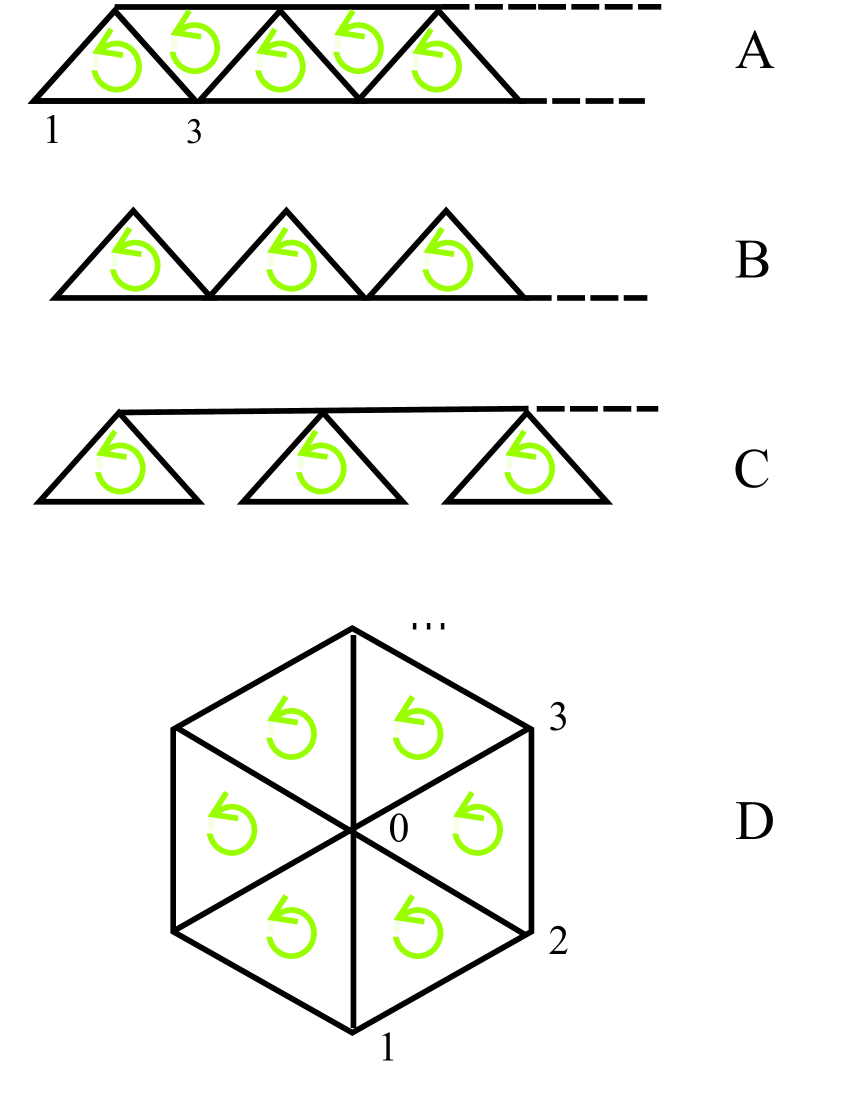
Figure 1: Quasi-1D geometries. The spins reside on the vertices and spin-spin interactions are represented by the edges. At each triangle there is also a chiral three-spin interaction which has the same sense everywhere, as indicated by the arrows.

For $|\lambda|\ll 1$, the ferromagnetic interaction dominates and spins align along any direction. For $|\lambda|\gg 1$, the chiral interaction dominates, the magnetic ordering disappears and we observe the establishment of chiral order in different plaquettes. Note that by fixing the sign of $X_{ijk}$ we impose the condition that all plaquettes have the same chiral orientation [See Fig. 1]. This leads to an additional frustration in the chiral regime and may prevent the system from achieving the largest value of the chirality, which is $2\sqrt{3}$ per plaquette, even for very large values of $\lambda$.

Let us now look at the different quasi-1D models. For the ladder of type A the nonzero couplings are

$$J_{i,i+1} = 1,$$ (6)

$$J_{i,i+2} = 1,$$

$$X_{i,i+1,i+2} = (-1)^{i},$$

where the factor $(-1)^{i}$ fixes the same orientation of the chiral term on all triangles. The ladder of type B is very similar, but the upper row of Heisenberg and half of the chiral interactions are missing, so that

$$J_{i,i+1} = 1,$$ (7)

$$J_{2i,2i+3} = 1,$$

$$X_{2i,2i+1,2i+2} = 1.$$

By contrast, the ladder of type C is formed by a set of weakly connected triangles, in which case we obtain

$$J_{i,i+1} = 1,\quad i=1,2,4,5\ldots$$ (8)

$$J_{i,i+2} = 1,\quad i=1,4,7,\ldots$$

$$J_{i,i+3} = 1,\quad i=2,5,8,\ldots$$

$$X_{i,i+1,i+2} = 1,\quad i=1,4,7,\ldots$$

Finally, in the ring-type geometry shown in Fig. 1(D) there is a central spin-$\frac{1}{2}$ particle (the spin labelled ‘0’) which is connected to $N-1$ equidistant spins. The Hamiltonian of this system is best written explicitly as

$$H_{\rm ring} = -\sum_{i=1}^{N}\vec{\sigma}_{0}\cdot\vec{\sigma}_{i}-\sum_{i=1}^{N-1}\vec{\sigma}_{i}\cdot\vec{\sigma}_{i+1}$$ (9)

$$+\lambda\sum_{i=1}^{N-1}\vec{\sigma}_{0}\cdot\vec{\sigma}_{i}\times\vec{\sigma}_{i+1}.$$

III.2 Analytic results

We have studied analytically these models, in order to get information about the ground state energies and the location of possible quantum phase transitions. We present in detail the method only for the type-A ladder, but the procedure is the same for the rest of the geometries. Our solution works in three steps (i) a mapping to a hard-core bosonic problem, (ii) a second mapping to a fermionic model and (iii) a mean-field solution of the fermionic model.

First of all, the spins are mapped onto bosons using the Dyson-Maleev transformation Sachdev ,

$$X_{n}=b_{n}+b^{\dagger}_{n},\;\;Y_{n}=-i(b_{n}-b^{\dagger}_{n}),\;\;Z_{n}=1-2b^{\dagger}_{n}b_{n}\;\;\;$$ (10)

where the $b,b^{\dagger}$ are bosonic operators that satisfy the commutation relations $[b_{n},b^{\dagger}_{m}]=\delta_{nm}$, and $[b_{n},b_{m}]=[b^{\dagger}_{n},b^{\dagger}_{m}]=0$. To be consistent with the spin-$\frac{1}{2}$ problem at hand, we allow up to one boson per lattice site, i.e., $b^{\dagger}_{n}b_{n}\leq 1$. In this representation the Heisenberg interaction between the $m$-th and $n$-th spins reads

$$\vec{\sigma}_{m}\cdot\vec{\sigma}_{n}=(1-2b^{\dagger}_{m}b_{m})(1-2b^{\dagger}_{n}b_{n})+2(b_{m}^{\dagger}b_{n}+b_{n}^{\dagger}b_{m})$$

while the chiral interaction between spins $l$, $m$ and $n$ becomes

$${\cal X}_{lmn} = 2i[(b_{m}^{\dagger}b_{l}-b_{l}^{\dagger}b_{m})(1-2b_{n}^{\dagger}b_{n})$$ (12)

$$+(b_{n}^{\dagger}b_{m}-b_{m}^{\dagger}b_{n})(1-2b_{l}^{\dagger}b_{l})$$

$$+(b_{l}^{\dagger}b_{n}-b_{n}^{\dagger}b_{l})(1-2b_{m}^{\dagger}b_{m})].$$

The next step is to turn to fermionic variables, $c_{n}$. We achieve this by using the Jordan-Wigner transformation

$$c_{n}=(-1)^{\zeta_{n}}b_{n},\quad\zeta_{n}=\sum_{k<n}c_{k}^{\dagger}c_{k}$$ (13)

where $\zeta_{n}$ gives the total number of fermions on the sites to the left of site $n$. These new operators satisfy fermionic anticommutation relations $\{c_{n},c^{\dagger}_{m}\}=\delta_{nm}$, and $\{c_{n},c_{m}\}=\{c^{\dagger}_{n},c^{\dagger}_{m}\}=0$. In addition to this we also need the following relations

$$b_{n}^{\dagger}b_{n}=c_{n}^{\dagger}c_{n},\quad b_{n}^{\dagger}b_{n+1}=c_{n}^{\dagger}c_{n+1},$$

$$b_{n}^{\dagger}b_{n+2}=c_{n}^{\dagger}(-1)^{c_{n+1}^{\dagger}c_{n+1}}c_{n+2}.$$ (14)

Replacing all formulas above into the particular Hamiltonian (5) one obtains a complicated fermionic model which in general has no simple analytical solution. We may nevertheless estimate variationally the properties of the ground state.

Our approximation method proceeds as follows. We notice that for $|\lambda|\ll 1$ one of the possible ferromagnetic ground states is polarized along the z-direction. This means that the state has no effective fermions and $\alpha\equiv\langle b^{\dagger}_{n}b_{n}\rangle=0$. It thus makes sense to treat $\alpha$ as our order parameter; to accurately find the phase transition the expression as a function of $\alpha$ must become exact in the limit of one boson, $\alpha={\cal O}(1/N)$, where the transition to the chiral regime occurs.

Our mean field method dictates two approximations. In the Heisenberg term we replace

$$(1-2c_{n}^{\dagger}c_{n})(1-2c_{m}^{\dagger}c_{m})\to 1+2(\alpha-1)(c_{n}^{\dagger}c_{n}+c_{m}^{\dagger}c_{m})$$ (15)

for the various pairs of interacting sites. In the chiral term we simply substitute $(2c_{i+2}^{\dagger}c_{i+2}-2c_{i-1}^{\dagger}c_{i-1})$ with 0, which leads to a cancellation of the diagonal hopping terms, leaving only the quadratic next-nearest-neighbor hopping. With this, the Hamiltonian of type-A ladder becomes

$$H_{\rm A}=-2N-2\sum_{l}\left[c_{l+1}^{\dagger}c_{l}+c_{l}^{\dagger}c_{l+1}-8(\alpha-1)c_{l}^{\dagger}c_{l}\right]$$ (16)

$$-2\sum_{l}\left\{[(1-2\alpha)+\lambda i(-1)^{l}]c_{l+2}^{\dagger}c_{l}+\mathrm{H.c.}\right\}.$$

It is now convenient to regroup the fermionic operators to form a spinor, $\Psi_{l}^{T}\equiv(c_{2l+1},c_{l})$, and then to perform a discrete Fourier transform

$$\Psi_{l}=\frac{1}{\sqrt{N}}\sum_{p}e^{ipl}\Psi_{p}$$ (17)

where $p=2\pi n/L$ for $n=0,1,\ldots(L-1)$ and $L=N/2$ is the length of the ladder. Consequently the Hamiltonian becomes

$$H_{\rm A}=-2N+\sum_{p}\Psi_{p}^{\dagger}M_{p}\Psi_{p}$$ (18)

with the coupling matrix

$$M_{p}=[8(1-\alpha)-4(1-2\alpha)\cos(p)]\mathbb{I}$$ (19)

$$-2[1+\cos(p)]\sigma_{x}-2\sin(p)\sigma_{y}-4\lambda\sin(p)\sigma_{z}.$$

The eigenvalues of the matrix yield the eigenenergies of the Hamiltonian, which are

$$E_{\pm}(p)=8(1-\alpha)-4(1-2\alpha)\cos(p)$$ (20)

$$\pm 2\sqrt{(4\lambda^{2}+1)\sin^{2}(p)+[1+\cos(p)]^{2}}.$$

If we label as $E_{k}$ the $2L$ eigenenergies, sorted such that $E_{k}\leq E_{k+1}$, the lowest energy state of our model has $\alpha N$ fermions occupying the states $k=1$ up to $k=\alpha N$. The energy is then given by $E=\sum_{k=1}^{\alpha N}$ and the right value of $\alpha$ is found by solving numerically the self-consistency equation

$$\alpha N=\sum_{E_{+}(p)\leq 0}1+\sum_{E_{-}(p)\leq 0}1.$$ (21)

This procedure can be repeated for all the lattice configurations shown in Fig. 1, obtaining again upper bounds for the energy of the ground state. In addition, we can compute the value of $\lambda$ at which the phase transition from the ferromagnetic ground state to the chiral state happens. This is given by the configuration at which $\alpha\neq 0$ becomes favorable, which is the configuration in which some $E_{\pm}(p)$ become negative.

III.3 Numerical results

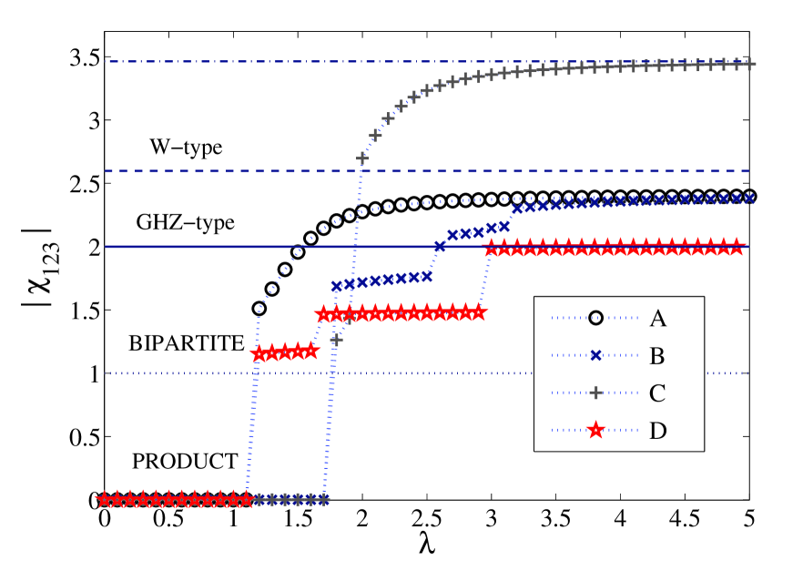
Figure 2: Absolute value of the chirality vs. strength of chiral interaction for the different geometries of Fig. 1 (for $N=9$ spins with periodic boundary conditions). We see that the chirality of lattice types A, B, C, and D becomes nonzero at the points $\lambda_{\rm A}\approx 1.1$, $\lambda_{\rm B}\approx 1.7$, $\lambda_{\rm C}\approx 1.7$, and $\lambda_{\rm D}\approx 1.1$, respectively. The horizontal lines (from top to bottom) correspond to the maximum chirality ($=2\sqrt{3}$), and the entanglement witnesses for W-like ($=3\sqrt{3}/2$), GHZ-like ($=2$) and bipartite entangled ($=1$) states, as demonstrated in Section II.

Figure 3: Ground state energy per lattice site vs. strength of chiral interaction for a type-A ladder (Fig. 1a). The solid line is the analytical estimate computed using the fermionization in Sect. III.2, while the dashed and dashed-dotted lines come from an exact diagonalization of the model for $N=7$ and $N=15$ spins, respectively.

In addition to the mean field studies, we have diagonalized exactly the Hamiltonian in Eq. (5) using all four geometries and an increasing number of spins. In all cases we observe a phase transition from a ferromagnetic regime ($\lambda=0$) to a chiral one ($|\lambda|\to\infty$). The location of the phase transition depends on the particular model and agrees with the estimates developed above. From the analytics, for the ladder of type A and for the ring geometry we find $\lambda_{\rm tran}\approx 1.1$, while for the two other configurations we have $\lambda_{\rm tran}\approx 1.7$. As shown in Fig. 2, these values are close to the actual location of the jumps in the chirality that are obtained numerically.

It is interesting to note that, in the chiral phase, the total chirality strongly depends on the geometry of the lattice. Since our Hamiltonian favors the same orientation of chirality on all plaquettes, the type-A ladder experiences a particular kind of frustration, where no two adjacent plaquettes are able to host maximal chiral currents. A similar phenomenon is experienced by the type-B lattice, but not by the type-C ladder, where the weakly connected plaquettes are able to saturate the maximum value of the chirality per site (cf. Fig. 2). On the other hand, the ring configuration appears to have only bipartite entanglement. This is due to rotational symmetry, which forces the central spin to decouple from each of the triangles, thus forbidding any possible tripartite correlations.

As we have seen, chirality acts as an entanglement witness for two- and three-partite entanglement. Following our previous analysis, and from Fig. 2, we conclude that plaquettes in the A and B ladders have genuine three-partite entanglement of GHZ-type. Ladder C, with its weakly bound triangles and no frustration, achieves W-type entanglement on every three neighboring spins.

We have compared the energies per site provided by the numerical simulation with the analytical mean-field results. As shown in Fig. 3, the derivative of the energy per site experiences a discontinuity around the transition point. This feature is shown both in the numerics and in the mean field estimates. The latter, however, only provide a variational upper bound that is approached by the numerical exact diagonalization for increasing number of spins.

We have also investigated numerically the spin-spin correlations of the ground state of type-A ladder for various ladder sizes and chiral couplings, $\lambda$, using periodic boundary conditions. A suitable way to measure the quantum correlations is to evaluate the connected correlator

$$C_{i,j}=\langle\vec{\sigma}_{i}\cdot\vec{\sigma}_{j}\rangle-\langle\vec{\sigma}_{i}\rangle\cdot\langle\vec{\sigma}_{j}\rangle$$ (22)

between any two spins. Scaling studies show that two different behaviors corresponding to the two phases of the system are obtained. Below the phase transition, $\lambda<\lambda_{\rm tran}\approx 1.1$, on the ferromagnetic regime, spins are completely aligned and the connected correlation becomes zero. Above the phase transition, in the chiral phase $\lambda>\lambda_{\rm tran}\approx 1.1$ the quantum spin-spin correlations appear to decrease exponentially fast with the separation of spins, $|i-j|$. Both regimes are shown in Fig. 4, where we plot the correlator $C_{0,\Delta}$ between the first and any other spin on a type-A ladder with $N=24$ sites. For $\lambda=0.2$ the correlator $C_{0,\Delta}$ is identically zero, while for $\lambda=100$ it becomes negligible beyond the sixth site. This demonstrates the absence of structure in the ground state of type-A ladder when it is in the chiral regime.

Figure 4: Spin-spin correlations $C_{0,\Delta}$ [Eq. (22)] for a periodic type-A ladder with $N=24$ spins. The dashed-dot line corresponds to $\lambda=0.2$ and the solid line to $\lambda=100$. In the chiral regime the correlations decay exponentially (on either direction of the periodic ladder).

IV Two-dimensional model

Rows $\times$ columns	$\left|S,S_{z}\right\rangle$	degeneracy
$2\times n$	$\left|0,0\right\rangle$	1
$3\times 3$	$\left|\frac{1}{2},\pm\frac{1}{2}\right\rangle$	4
$3\times 4$	$\left|0,0\right\rangle$	1
$3\times 5$	$\left|\frac{1}{2},\pm\frac{1}{2}\right\rangle$	4
$4\times 4$	$\left|0,0\right\rangle$	1
$4\times 5$	$\left|0,0\right\rangle$	1

Table 2: Properties of the ground state in the chiral phase, $|\lambda|\gg 1$, for various lattice sizes. We show the magnetization, $S_{z}$, the total spin, $S$, and the degeneracy of the ground state.

In this section we consider the two dimensional triangular lattice and impose periodic boundary conditions in both directions. The lattice is represented by an array, as illustrated in Fig. 6, with dimensions denoted as N times M. We have performed exact numerical diagonalization of the Hamiltonian for various sizes of the lattice and characterized both the ground state and its lowest excitations.

The results are summarized in Table 2 and in Fig. 5. Once more, we obtain two phases separated by a phase transition point at a position that approaches $\lambda_{\rm tran}\approx 1.1$ for large lattices. When the chiral coupling $\lambda$ is small ($\lambda<\lambda_{\rm tran}$) then the Heisenberg interaction is dominant and the system is in a ferromagnetic state. When the coupling is large ($\lambda>\lambda_{\rm tran}$) then the chiral term is dominant causing the ground state to have non-zero chirality (see Fig. 5(a). Connecting with our studies of the chirality as an entanglement witness, the larger degree of frustration in the toric setup prevents the system from reaching a large value of the chirality, which lays around $1.5$ in the limit $|\lambda|\to\infty$. This implies that the state belongs to the set of states which are at least two-party entangled.

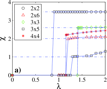
Figure 5: (a) Ground state mean chirality as a function of the coupling constant $\lambda$ for different lattice sizes. (b) Energy gap between the ground state and the first excited state.

The existence of the quantum phase transition and even its location agree qualitatively with the features of the Type A ladder, whose geometry most closely resembles that of these toric structures. However, as we show below, there are some differences. The most notable one is in the angular momentum of the ground state. We have found that in the chiral phase the system tends to adopt the state with the lowest total angular momentum which is compatible with the number of spins. Thus, as shown in Table 2, if the number of spins is even, which includes the case of Type A ladders, the ground state is a state with $S=0$ and $S_{z}=0$ and has no degeneracy. The corresponding momentum of the ground state is zero. However, if the total number of spins is odd, the total angular momentum must be fractional, having $S=\frac{1}{2}$ and $S_{z}=\pm\frac{1}{2}$. In this case the ground state becomes four-fold degenerate distinguished by the $z$ component of the spin and by the momentum which is either zero or $\pi$ in both directions.

It is interesting to note that the excited states almost always have a larger angular momentum and are separated by a large energy gap, ${\cal O}(|\lambda|)$, from the ground state. This is illustrated in Fig. 5(b). This energy gap, which survives in the thermodynamic limit, is responsible for a finite correlation length. This causes both the spin-spin and chiral-chiral correlations to die off exponentially fast (see Fig. 4 for the spin-spin correlations in the case of a type-A ladder).

Remarkably, on some special cases, such as the $3\times 5$ lattice, the gap between the ground and excited states is much smaller (see Fig. 5(b)). The excited states then have similar values of total angular momenta and their chiralities differ only slightly — by $0.2$ or less — from that of the ground state. We conjecture that the existence of these states is supported by the frustration of the chirality in Eq. (2) where we enforce all plaquettes to have a similar orientation of the spin current.

The chiral-chiral correlations are presented in Fig. 6 for a $4\times 4$ lattice, where we show the connected correlation

$$\langle{\cal XX}\rangle\equiv\langle{\cal X}_{ijk}{\cal X}_{lmn}\rangle-\langle{\cal X}_{ijk}\rangle\langle{\cal X}_{lmn}\rangle$$ (23)

between a reference plaquette $(lmn)$ and any other one, $(ijk)$. In Fig. 6(a) the reference plaquette is given by the sites $(2,2)$, $(2,3)$ and $(3,3)$ of the $4\times 4$ lattice. The value of $\langle{\cal XX}\rangle$ between the reference site and itself is $7.042$, while the connected correlation with respect to neighboring triangles decreases dramatically. This indicates the absence of any structure in the chirality of the ground state.

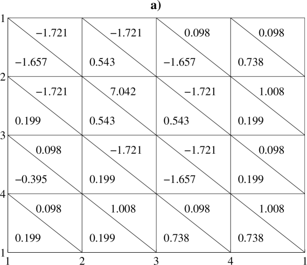
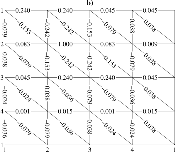
Figure 6: A geometrical configuration of the $4\times 4$ periodic lattice. The position $(n,m)$ of the site on the lattice is given in terms of the integers $n,m=1,...,4$. A certain bond is depicted as $(n,m)-(k,l)$ that connects the corresponding two neighboring sites. (a) Chiral correlation between the plaquette with sites $(2,2)$, $(2,3)$ and $(3,3)$ and the remaining ones. Note the difference between the value of $\langle{\cal XX}\rangle$ for the same plaquette ($7.042$) and neighboring ones. (b) Dimer correlations between the bond $(2,2)-(2,3)$ and the remaining bonds. The simulations were performed deep in the chiral regime $|\lambda|=100$.

The structure of the ground state is a singlet whenever the total number of spins is even. This by itself does not necessarily imply a complicated hidden order, since we could achieve the same value of the total angular momentum by packing the spins into singlets. Following Ref. misguich98 we have computed the dimer order parameter, which is defined as the connected correlation of an operator $d_{ij}=(1-\vec{\sigma}_{i}\cdot\vec{\sigma}_{j})/4$ that detects singlets. The dimer-dimer correlations are then defined as

$$D_{ij}=\frac{\langle d_{ij}d_{kl}\rangle-\langle d_{ij}\rangle\langle d_{kl}\rangle}{\langle d_{kl}\rangle(1-\langle d_{ij}\rangle)},$$ (24)

where $(kl)$ is the reference bond and $(ij)$ any other bond. In our case the value of the dimer order $D$ decreases rapidly as a function of the bond separation (see Fig. 6a), suggesting that this is not a dimer solid.

Summarizing, the ground state of the $4\times 4$ periodic lattice appears to have no structure with respect to spin-spin correlations or chirality-chirality correlations. Moreover, the dimer correlations appears to reduce dramatically for increasing distance between the dimers.

V Optical lattice implementation

Here we would like to sketch a method of how to produce the Heisenberg and chiral interactions studied in this paper by employing cold atoms superposed with optical lattices. More precisely we consider a Mott insulator of two species bosonic atoms loaded on an optical lattice with a triangular configuration, as shown in Fig. 7. These two states can be encoded in the internal hyperfine states of an atom. In the limit of deep off-resonance optical lattices, the evolution of this system is described by a Bose-Hubbard Hamiltonian for atoms of species ${\cal S}=a,b$

$$H = -\sum_{i,{\cal S}}(J^{{\cal S}}_{i}a_{i,{\cal S}}^{\dagger}a_{i+1,{\cal S}}+{\rm H.c.})$$ (25)

$$+ \frac{1}{2}\sum_{i,{\cal S}}U_{{\cal S},{\cal S}}n_{i,{\cal S}}(n_{i,{\cal S}}-1)+\sum_{i}U_{a,b}n_{i,a}n_{i,b}$$

Here $J^{S}>0$ is the atom tunnelling coupling between neighboring sites, $U_{S,S^{\prime}}$ is the on-site interaction between atoms $S$ and $S^{\prime}$, $a_{i,{\cal S}}$ denotes the annihilation operator of atoms of species ${\cal S}$ at the site $i$ and $n_{i,{\cal S}}$ is the corresponding number operator. For simplicity we take $U_{S,S^{\prime}}$ to be positive.

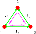
Figure 7: The triangular configuration. Three-spin interaction terms appear between sites $1$, $2$ and $3$ since tunnelling between two of the sites, such as $1$ and $2$, can happen directly or through the third site. The latter case results into an exchange interaction between $1$ and $2$ that is influenced by the state of the spin at site $3$.

As we are interested in a chiral interaction we want to generate an effective charge-magnetic field coupling in the atomic system manifested by complex, position dependent, tunnelling couplings. For example, it has been shown in Refs. Pachos ; Kay ; Pachos_Rico that a gradient of a magnetic field along the direction of the electric dipole moment can simulate effectively the interaction between a charge and a homogenous magnetic field. Alternatively, Raman assisted tunnelling with lasers that have a phase difference Jaksch can be also employed. We will employ such a technique here to generate, in a controlled way, complex position dependent tunnelling couplings.

In the insulator regime, hopping is weak compared to the interaction, $J\ll U$, and atoms have a low probability of jumping to other sites. For populations of only one atom per lattice site we can employ the pseudo-spin basis for each lattice site, given by $|n_{a}=1,n_{b}=0\rangle\equiv|\!\!\uparrow\rangle$ and $|n_{a}=0,n_{b}=1\rangle\equiv|\!\!\downarrow\rangle$. In that limit one can treat the hopping terms perturbatively and find that they help to establish effective exchange interactions between atoms in neighboring sites. Up to third order in the perturbation expansion the effective Hamiltonian is given by

$$H = \alpha\sum_{i}I\!\!I+\beta\sum Z_{i}+\gamma\sum_{i}Z_{i}Z_{i+1}$$ (26)

$$+ \delta\sum_{i}(X_{i}Y_{i+1}-Y_{i}X_{i+1})$$

$$+ \epsilon\vec{\sigma}_{i}\cdot\vec{\sigma}_{i+1}\times\vec{\sigma}_{i+2}$$

The presented couplings are given by

$$\alpha=\frac{{J^{a}}^{2}}{U_{aa}}+\frac{{J^{b}}^{2}}{U_{bb}},\,\,\,\,\,\beta=\frac{{J^{a}}^{2}}{2U_{aa}}-\frac{{J^{b}}^{2}}{2U_{bb}}$$

$$\gamma=\frac{{J^{a}}^{2}}{U_{aa}}+\frac{{J^{b}}^{2}}{U_{bb}},\,\,\,\,\,\delta=i\left(\frac{{J^{a}}^{2}J^{b}}{2U_{aa}^{2}}+\frac{{J^{b}}^{2}J^{a}}{2U_{bb}^{2}}\right)$$

$$\epsilon=i\left(\frac{{J^{a}}^{2}J^{b}}{2U_{aa}^{2}}-\frac{{J^{b}}^{2}J^{a}}{2U_{bb}^{2}}\right).$$

If we choose $J^{b}$ to be a negative imaginary number then it is possible to set $\alpha$, $\gamma$ and $\delta$ equal to zero. In addition, we can apply an effective magnetic field that cancels the $\beta$ term, resulting eventually to an isolated $\epsilon$ term,

$$H=\epsilon\sum_{i}\vec{\sigma}_{i}\cdot(\vec{\sigma}_{i+1}\times\vec{\sigma}_{i+2}).$$ (27)

This is the chiral interaction that we required.

The presented interaction is produced from third order perturbation theory and it could be rather small PachosKnight . A similar interaction can be engineered using recently developed techniques that involve cold molecules in optical lattices Zoller . Compared to the cold atom implementation shown here, the molecules would have the advantage of producing stronger interactions.

VI Conclusions

In this article we have studied a chiral spin system which is defined on a two dimensional triangular lattice. The analytical or numerical study of the 2D-model is hard so we initially resorted to simplified geometries such as triangular ladders and polygons (Fig. 1). By fermionizing and using mean field approximation we obtained the transition points, that separate between a spin-ordered and a chiral phase, as well as an upper bound for the ground state energies. These are in agreement with exact diagonalization of finite size systems (see Figs. 2, 3). From these results we have observed that for the ladder of type A the phase transition happens for smaller values of the chiral coupling $\lambda$, compared to the corresponding transition points for cases B and C. This has been attributed to frustration effects that also arise in the two dimensional case. On the contrary, case C has chirality that saturates the upper bound $\chi\leq 2\sqrt{3}$, for large chiral coupling $\lambda$. Moreover, case A and the 2D-lattice saturate to a lower value of the chirality. Using the chirality as a witness of entanglement, we have discussed the entanglement properties of the system and distinguished between two-party and genuine three-party entanglement. We have suggested that the recent advances in cold atom and polar molecule technologies Pachos ; Kay ; Pachos_Rico ; Jaksch ; Zoller could facilitate the experimental realization of the chiral systems presented here.

The study of topological order is rather complex and its presence in actual physical systems is hard to probe in a definitive way. Moreover, finite size simulations make it possible to deduce certain characteristics which can only indicate the presence of topological order. Indeed, the extensive numerical calculations carried out here on the 2D model suggest the presence of topological order in the ground state of the system, which has been supported by a number of observations. Firstly, the system exhibits a ground state degeneracy that goes beyond the breaking of the PT-symmetry. Secondly, there is an energy gap between the ground and the excited states, which persists with increasing lattice size. Finally, in the chiral regime the two-point spin correlations, the chiral connected correlation and the dimer correlations appear to decay exponentially, a behavior that indicates the absence of any local structure in the ground states.

- (1) X.-G. Wen, Quantum Field Theory of Many-Body Systems (Oxford University Press, 2004).
- (2) R.B. Laughlin, Phys. Rev. Lett. 50, 1395 (1983).
- (3) X.-G. Wen, F. Wilczek, A. Zee, Phys. Rev. B 39, 11413 (1989).
- (4) X.-G. Wen and Q. Niu, Phys. Rev. B 41, 9377 (1990).
- (5) X.-G. Wen, Phys. Rev. B 65, 165113 (2002).
- (6) A. Kitaev and J. Preskill, Phys. Rev. Lett. 96, 110404 (2006); M. Levin and X.-G. Wen, ibid. 96, 110405 (2006).
- (7) C. Lhuillier, Frustrated quantum magnets, cond-mat/0502464.
- (8) Y. Taguchi, Y. Oohara, H. Yoshizawa, N. Nagaosa, Y. Tokura, Science 291, 2573 (2001).
- (9) D. Grohol, K. Matan, J.H. Cho, S.-H. Lee, J.W. Lynn, D.G. Nocera, Y.S. Lee, Nature Materials 4, 323 (2005).
- (10) J.K. Pachos, Phys. Lett. A 344, 441 (2005).
- (11) A. Kay et al., Optics and Spectroscopy 99, 355-372 (2005).
- (12) J.K. Pachos and E. Rico, Phys. Rev. A 70, 053620 (2004).
- (13) D. Jaksch and P. Zoller, New J. Phys. 5, 56 (2003).
- (14) H.P. Büchler, A. Micheli, P. Zoller, Nature Physics 3, 726 (2007).
- (15) W. Dür, G. Vidal, and J. I. Cirac, Phys. Rev. A 62, 062314 (2000).
- (16) S. Hill and W.K. Wootters, Phys. Rev. Lett. 78, 5022 (1997).
- (17) M. Horodecki, P. Horodecki and R. Horodecki, Phys. Lett. A 223, 1 (1996).
- (18) G. Toth & O. Gühne, Phys. Rev. Lett. 94, 060501 (2005).
- (19) S. Sachdev, Quantum Phase Transitions, Cambridge University Press (2001).
- (20) G. Misguich, C. Lhuillier, B. Bernu and C. Waldtmann, Phys. Rev. Lett. 81, 1098 (1998); G. Misguich, C. Lhuillier, B. Bernu and C. Waldtmann, Phys. Rev. B 60, 1064 (1999).
- (21) J. K. Pachos and P. L. Knight, Phys. Rev. Lett. 91, 107902 (2003).