Boltzmann equation approach to transport in finite modular quantum systems

Abstract

We investigate the transport behavior of finite modular quantum systems. Such systems have recently been analyzed by different methods. These approaches indicate diffusive behavior even and especially for finite systems. Inspired by these results we analyze analytically and numerically if and in which sense the dynamics of those systems are in agreement with an appropriate Boltzmann equation. We find that the transport behavior of a certain type of finite modular quantum systems may indeed be described in terms of a Boltzmann equation. However, the applicability of the Boltzmann equation appears to be rather limited to a very specific type of model.

I Introduction

There are essentially two major tools which are used to analyze the transport behavior of quantum systems: Linear response theory as implemented in terms of the Kubo formula Kubo ; mahan ; Klu ; Zotos ; Heidr ; Jung , and approaches based on the Boltzmann equation (BE) Boltzmann . The validity of the latter has been subject to ongoing discussions during the last century boltzmann2 . This refers to the BE as a method to describe gas-dynamics on purely classical grounds. In the context of quantum mechanics the situation may even be more complicated. Can the dynamics of systems that are controlled by the Schrödinger equation (SE) be mapped on a BE? And if so, how? Considerable work in that direction has been done by Peierls Peierls , Kadanoff, Baym baym and others keldysh ; winkel ; Kohn . In this literature it is frequently pointed out that the mapping typically relies on additional assumptions like the “random phase approximation” Peierls or the possibility to truncate graphic expansions that does not necessarily follow from the underlying dynamics baym . But also recent publications address the mapping of quantum dynamics onto BE’s spohn ; Horny ; vacchi . In the article at hand we investigate the applicability of a BE to systems which are both, complex enough to exhibit diffusive behavior and simple enough to be analyzed from first principles by direct numerical integration. Thus the dynamics as resulting from a BE may simply be compared to the dynamics as resulting from the SE. The results for transport behavior of those systems obtained by other methods (Kubo formalism, Hilbert space average method (HAM), time-convolutionless (TCL) Buch ; TCL ; JG , which have been mentioned in the abstract, may be found in heat ; kubop ; chaos ; Breu

The article at hand is organized as follows:
In Sect. II we very briefly review the concepts underlaying the famous BE which is meant to be a gross description of the dynamics of dilute gases. We comment on linear forms of the BE and their diffusive solutions, i.e., we state an explicit form for the diffusion coefficient. In Sect. III we introduce our finite modular quantum system which may be viewed as model for a particle hopping between a few lattice sites or a model for the energydynamics within a chain of, e.g., molecules. The main intention of the work at hand is to investigate the transport behavior of finite quantum systems by means of an analysis based on the BE. To those ends we propose to identify the classical particle densities which appear in the BE with the the quantum mechanical occupation numbers of current eigenstates (IV). To justify this concept we numerically and analytically analyze in Sect. V whether the dynamics of the current occupation numbers are indeed well described by an appropriate linear BE. This turns out to be the case but only for a quite specific form of the interactions within the model. For this type on interactions we concretely compute the adequate linear BE and determine the diffusion coefficient using the form given in Sect. II. This coefficient turns out to be in accord with the results from the different approaches to similar systems mentioned above heat ; kubop ; chaos . An ab initio numerical analysis of the full dynamics of the quantum system (including lattice site occupation numbers) shows that it indeed exhibits diffusive behavior controlled by the above diffusion coefficient. In the last Sect. we discuss the dependence of those results on special properties of our model.

II Boltzmann equation and diffusive solutions

As wellknown, in 1872 Boltzmann undertook to explain the macroscopic dynamics of dilute gases. For the description of a gas Boltzmann introduced the ${\bf\mu}$-space, which is essentially a one-particle phase space. An $N$-particle gas would thus technically be represented by $N$ points in ${\bf\mu}$-space rather than one point in standard Hamiltonian phase space. But instead of using $N$ points in ${\bf\mu}$-space for the description of the gas, Boltzmann introduced a distribution function $\Phi({\bf r},{\bf v},t)$ in a somewhat ”coarse-grained” ${\bf\mu}$-space which is supposed to give the number of particles being in a -space cell around $d^{3}rd^{3}v$:=$dxdydzdv_{x}dv_{y}dv_{z}$. Instead of trying to describe the motion of every single particle (which is impossible due to the huge numbers of particles in a gas) Boltzmann suggested his famous equation which describes the time evolution of $\Phi({\bf r},{\bf v},t)$ in $\mu$-space and is, in the absence of any external force, given by:

$$\frac{d}{dt}\Phi({\bf r},{\bf v})={\bf v}\cdot\nabla_{{\bf r}}\Phi({\bf r},{\bf v})+\dot{\Phi}({\bf r},{\bf v})_{scatt},$$ (1)

The first expression on the right-hand-side is supposed to account for the dynamics due to particles that do not collide, whereas $\dot{\Phi}({\bf r},{\bf v})_{scatt}$ describes the dynamics arising from collisions. Those dynamics are only taken into account in terms of the transition rates $R$ and the (coarse grained) particle densities $\Phi$, neglecting all correlations and structures on a finer scale. Thus this type of dynamics implement the famous “assumption of molecular chaos” or the so-called “Stoßzahlansatz”. (According to the Stoßzahlansatz particles are not correlated before collisions, even though they get correlated by collisions, due to very many intermediate collisions before the same particles collide again). However, this treatment of collisions introduces the irreversibility into the BE that is not present in the underlying Hamiltonian equations.
If either $\Phi$ is close to equilibrium or for systems in which particels only collide with external scattering centers (no particle-particle collisions), the BE takes on the following linear form.

$$\dot{\Phi}({\bf r},{\bf v})+{\bf v}\cdot\nabla_{{\bf r}}\Phi({\bf r},{\bf v})=\int R({\bf v},{\bf v^{\prime}})\Phi({\bf r},{\bf v^{\prime}})d{\bf v}^{\prime},$$ (2)

A “velocity discretized” version of this linear BE reads

$$\dot{\Phi}_{i}({\bf r})+{\bf v}_{i}\cdot\nabla_{{\bf r}}\Phi_{i}({\bf r})=\sum_{j}R_{ij}\Phi_{j}(\bf r),$$ (3)

where the matrix of rates $R_{ij}$ is of the standard form as appearing in master equations. (It is this discrete linear BE which we are eventually going to use to describe our quantum system.)
As wellknown, in the limit of small density gradients (“long wavelength hydrodynamic modes”) (3) may feature diffusive solutions, i.e., solutions that fulfill

$$\dot{\rho}({\bf r})=\kappa\Delta\rho({\bf r}).$$ (4)

where the particle density $\rho({\bf r})$ is given by

$$\rho({\bf r})=\sum\limits_{i}\Phi_{i}({\bf r})$$ (5)

The diffusion coefficient in (4) takes on the form

$$\kappa=-\sum_{i,j}v_{i}R^{-1}_{ij}v_{j}\Phi^{0}_{j}.$$ (6)

$\Phi^{0}_{j}$ is the equilibrium velocity distribution (i.e., the solution of $R_{ij}\Phi^{0}_{j}=0$, accordingly called “null-space”). $R^{-1}_{ij}$ denotes the inverse of the rate matrix but without the null-space Balescu ; Brenig . (In the absence of any external scatterers $\kappa$ may diverge, indicating that no diffusive bahavior can be expected.)

III Definition of the model and its diffusive behavior

The systems we investigate in the following are called “finite modular quantum systems”. (This type of system has also been investigated inheat ; kubop ; chaos ). Those systems are essentially meant to allow for an investigation of transport behavior from first principles rather than to model some material or real physical system in great detail. Their total Hamiltonians may be written as

$$\hat{H}=\sum_{\mu=1}^{N}\hat{h}(\mu)+\sum_{\mu=1}^{N}\hat{V}(\mu,\mu+1),\qquad\text{with}\quad N+1\widehat{=}1$$

where $\hat{h}(\mu)$ denotes the local Hamiltonian of a subunit $\mu$, $\hat{V}(\mu,\mu+1)$ a next-neighbor interaction between subunits of the ring and $N$ the total number of subunits in the system.

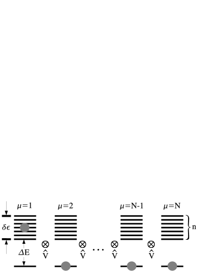
Figure 1: Sketch of the systems which are investigated for transport: N identical weakly coupled subsystems with a non- degenerate ground state and a band of equidistant energy levels.

A model which can be described by such a Hamiltonian is illustrated in Fig. 1. It consists of $N$ identical subsystems where each subunit features a nondegenerate ground state, a wide energy gap ($\Delta E$) and an energy band ($\delta\epsilon$) which contains $n$ equidistant energy levels. The local Hamiltonian is defined by

$$\hat{h}(\mu)=\sum\limits_{i=0}^{n+1}E_{i}\hat{\sigma}^{\dagger}_{i}(\mu)\hat{\sigma}_{i}(\mu) E_{i}=E_{0}+\Delta E+i\frac{\delta\epsilon}{n},$$ with (8)

for $$i\neq 0$$

and $\hat{{\sigma}}_{i}(\mu)=|0,\mu\rangle\langle i,\mu|$. Here $|0(i),\mu\rangle$ denotes the ground state (i’th level of the excitation band) of the $\mu$’th subunit. The interaction is specified by

$$\hat{V}(\mu,\mu+1)=\lambda\sum_{i,j=1}^{n}\tilde{V}_{ij}\hat{\sigma}^{\dagger}_{i}(\mu)\otimes\hat{\sigma}_{j}(\mu+1)+\text{h.c.}.$$ (9)

(h.c. denotes the hermitian conjugate of the previous sum). The $\tilde{V}_{ij}$ are complex numbers which are assumed to be adequately normalized such that $\lambda$ controlls the overall interaction strength. The choice of these $\tilde{V}_{ij}$ concretely determines the model. In heat ; kubop ; chaos the $\tilde{V}_{ij}$ are simply chosen to be independent random numbers (with mean zero) which leads to diffusive dynamics (in a sense explained below). In the paper at hand it turns out that this choice does not yield dynamics which are in accord with a BE. In fact, we will explain in Sect. V that it is only a rather specific choice which produces this accordance. However, at this point we do not specify the $\tilde{V}_{ij}$ any further.

Irrespective of the choice for the $\tilde{V}_{ij}$ the system may be viewed as a very simplified model for, e.g., a chain of coupled molecules or quantum dots, etc. In this case the hopping of the excitation from one subunit to another corresponds to energy transport. It may as well be viewed as a tight-binding model for particles on a lattice (in second quantization). There are, however, many ($n$) bands (orbitals per site) but no particle-particle interaction in the sense of the Hubbard-model (cf. (III), (9)). Thus one may characterize this model as a “single-particle multi-band quantum wire” with possibly random (interband) hoppings. Nevertheless, due to the independence of $\tilde{V}_{ij}$, $E_{i}$ of $\mu$ these are systems without disorder in the sense of, say, Anderson Anderson . (Note that the “total particle number” $\hat{N}:=\sum_{i,\mu}^{n,N}\hat{\sigma}^{\dagger}_{i}(\mu)\hat{\sigma}_{i}(\mu)$ is conserved)
We define diffusive transport for this model based on the evolution of expectation values $q_{\mu}(t)=\langle\Psi(t)|\hat{q}(\mu)|\Psi(t)\rangle$ of local fractions of some (globally conserved) quantity like energy or particle number ($|\Psi(t)\rangle$ denotes the systems full state). I. e., one may consider energy transport: $\hat{q}(\mu)=\hat{h}(\mu)$ or particle transport: $\hat{q}(\mu)=\hat{n}(\mu)=\sum_{i=1}^{n}\hat{\sigma}_{i}^{\dagger}(\mu)\hat{\sigma}_{i}(\mu)$., etc. We will call the transport diffusive if those local expectation values obey

$$\dot{q}_{\mu}(t)=\kappa\cdot\left(q_{\mu+1}(t)+q_{\mu-1}(t)-2q_{\mu}(t)\right),$$ (10)

which is a discrete version of the diffusion equation (4). In this case obviously only the diffusion coefficient $\kappa$ remains to be computed. If “diffusivity” is supposed to be a property of a system (10) has to apply of course to the largest part of all initial states under consideration.

IV Choice of quasiparticles for modelling transport

It is not a priory clear which quantum observable could play the role of a classical particle density in phase space when one attempts to map the quantum dynamics of some system onto a BE. A minimum requirement is surely the clear correspondence to some velocity
In the context of heat transport through electrically isolating crystals one identifies the particle (phonon) density with the average occupation number of a phonon mode. The velocity is then extracted from the phonon dispersion relation baym ; Peierls . However, the phonons are eigenmodes of a harmonic chain (spring-and-ball-model), and the scattering arises from a (weak) anharmonic part of the interaction. In our model the interactions do not allow for a decomposition into an harmonic and an anharmonic part. Thus this scheme cannot be applied here.
In the context of particle transport through systems of interacting particles in periodic lattices, the (quasi)particle density is basically identified with the occupation number of eigenmodes (Bloch waves) of the interaction-free particle, e.g., the crystal electron. The velocity (group velocity) is then computed from the corresponding dispersion relation . Since our model (from a “Hubbard” point of view) features no particle-particle interaction such a description would result in a BE without any scattering at all ($R_{ij}=0$), hence in ballistic transport. This however is not in accord with our findings (see below).
Thus, here we suggest to identify the particle density with the occupation number of eigenmodes of a suitable current operator. To define a current operator on the basis of the transported quantity we consider the time evolution of the corresponding local operator $\hat{q}(\mu)$ at site $\mu$ which is given by the Heisenberg equation of motion Klu ; Heidr ; Jung ; Michi :

$$\frac{d}{dt}\hat{q}(\mu) = \frac{\partial}{\partial t}\hat{q}(\mu)+\frac{{\bf i}}{h}\left[\hat{H},\hat{q}(\mu)\right]=\frac{{\bf i}}{h}\left[\hat{H},\hat{q}(\mu)\right],$$

since the operators $\hat{q}(\mu)$ mentioned above are explicitly time independent. After inserting equation (III) and applying the explicit form of $\hat{q}(\mu)(=\hat{h}(\mu),\hat{n}(\mu))$ we obtain:

$$\frac{d}{dt}\hat{q}(\mu)=\frac{{\bf i}}{h}\left[\hat{V}(\mu-1,\mu),\hat{q}(\mu)\right]+\frac{{\bf i}}{h}\left[\hat{V}(\mu,\mu+1),\hat{q}(\mu)\right].$$

(12)

If conserved quantities $q(\mu)$ are considered, currents are routinely defined on the basis of the temporal change of the respective densities by means of a (discrete) continuity equation which reads for $\hat{q}(\mu)$:

$$\frac{d}{dt}\hat{q}(\mu)=\hat{j}(\mu,\mu+1)-\hat{j}(\mu-1,\mu)=-\text{div}\hat{j}.$$ (13)

Comparing Eq.(12) with Eq.(13) this suggests the definition of a local current operator

$$\hat{j}^{Q}(\mu,\mu+1)=\frac{{\bf i}}{h}\left[\hat{V}(\mu,\mu+1),\hat{q}(\mu)\right],$$ (14)

whereas the total currentoperator $\hat{J}^{Q}$ is given by

$$\hat{J}^{Q}=\sum\limits_{\mu=1}^{N-1}\hat{j}^{Q}(\mu,\mu+1)=\frac{{\bf i}}{\hbar}\sum\limits_{\mu=1}^{N-1}\left[\hat{V}(\mu,\mu+1),\hat{q}(\mu)\right]$$ (15)

E.g., in the case of energy transport the current operator is

$$\hat{J}^{H}=\frac{{\bf i}}{\hbar}\cdot\lambda\sum\limits_{\mu=1}^{N-1}\sum\limits_{i,j}^{n}E_{i}\tilde{V}_{ij}\hat{\sigma}_{i}^{\dagger}(\mu)\otimes\hat{\sigma}_{j}(\mu+1)+\text{h.c.}.$$ (16)

Since the current is a product of velocity and density we assign a velocity to our quasiparticles by the relation

$$v_{n}=\frac{j^{Q}_{n}}{\langle j^{Q}_{n}|\hat{Q}|j^{Q}_{n}\rangle}\quad\text{with}\quad Q=\sum\limits_{\mu=1}^{N}\hat{q}(\mu),$$ (17)

where $j^{Q}_{n}$ is an eigenvalue of the corresponding current operator. In this way the velocities that eventually appear in (6) may be defined.

V Analysis of the dynamics of the model

In this Sect., we analyze whether the above described choice of quasiparticles is in accord with a BE from a dynamical point of view. Or, to formulate concise questions: May the dynamics of the populations of the current eigenmodes as resulting from the Schrödinger-dynamics of the quantum model be described in terms of an adequate BE? And if so what would be the rates in the scattering term?
In Sect. IV we suggested to identify the particle density as appearing in the BE by a quantity that corresponds to a specific velocity but not to a spatial coordinate. This is obviously in some sense insufficient since particle densities in phase space are labeled by velocity and poisition. However, since the model features translational invariance, the current eigenmodes (the populations of which are supposed to correspond to the particle densities) stretch uniformly over the full model. Thus the dynamics of their populations may be expected to possibly correspond to the dynamic as resulting from a BE for particle densities that are uniform with respect to the position coordinate, i.e., $\nabla_{\bf r}\Phi=0$. In this case particle densities are only labled by velocities and may directly be identified with current eigenstate populations. In the above mentioned case, (3) simplifies to

$$\dot{\Phi}_{n}(t)=\sum_{m}R_{nm}\Phi_{m}(t).$$ (18)

The above equation (18) yields exponential decay for the $\Phi$’s (possibly with various relaxation times). In the following we investigate whether the same behavior results from the SE for the current eigenmode populations i.e., if we compute $\Phi_{n}(t)$ from the definition $\Phi_{n}$:=Tr$\left\{\hat{\rho}(t)\hat{P}_{n}\right\}$ where $\hat{P}_{n}=|j_{n}\rangle\langle j_{n}|$ is the projector onto the subspace spanned by the current eigenstate $|j_{n}\rangle$. If this is the case the SE and the BE may be in accord. However, this question is hard to answer in general without using numerical reasoning, since otherwise the quantum dynamics for $\Phi_{n}(t)$ cannot be found. Thus, rather than analyzing the dynamics of the $\Phi_{n}(t)$’s themselves, we analyze a function of those that can be estimated without using numerics. Strictly speaking this of course means we go from a proof to a check of consistency (However, we also check dynamics of the $\Phi_{n}$ also directly numerically). This function we call $\mathcal{C}(t)$ and construct it as

$$\mathcal{C}(t)=\sum_{n}j_{n}\cdot\text{Tr}\left\{\hat{\rho}(t)\hat{P}_{n}\right\}=\text{Tr}\left\{\hat{J}\hat{\rho}(t)\right\},$$ (19)

It is obviously just a weighted sum of the $\Phi_{n}(t)$’s. If its dynamics are in accord with (18), $\mathcal{C}(t)$ should also decay exponentially. As (19) shows, $\mathcal{C}(t)$ is simply the current expectationvalue. In the Heisenberg picture the latter reads $\mathcal{C}(t)=$Tr$\left\{\hat{J}(t)\hat{\rho}(0)\right\}$. Again, we cannot analyze this in full generality, thus we specialize to a concrete initial state, which is sometimes called a “deviation density matrix”. It is given by $\hat{\rho}(0)=d^{-1}\cdot\hat{{\bf 1}}+\epsilon\hat{J}(0)$ ($\hat{{\bf 1}}$ = identity, $d$ = dimension of the corresponding (sub-)space) and fulfills the relation Tr$\left\{\hat{\rho}_{0}\right\}=1$ for density operators due to the fact that the current operator is traceless. Thus we obtain $\mathcal{C}(t)=\epsilon\cdot$Tr$\left\{\hat{J}(t)\hat{J}(0)\right\}$, which is simply the current-autocorrelation function. Without going into any detail here we should mention that, following concepts based on the Hilbert space average method (HAM) as presented in kubop ; JG ; Breu , $\mathcal{C}(t)$ can be expected to reasonably describe the evolution of the expectation value of the current for almost any initial state. Thus the results which will be derived analytically below can safely be expected to apply to a much larger class of initial states than covered by the deviation density matrix. Especially the results can be expected to apply to the largest part of all pure states, which is the class of states which will be primarily analyzed numerically below.
The current-autocorrelation function reads:

$$\tilde{\mathcal{C}}(t)=\sum\limits_{\alpha,\beta=1}^{n}|\langle\alpha|\hat{J}(0)|\beta\rangle|^{2}e^{-\frac{{\mathbf{i}}}{\hbar}(E_{\alpha}-E_{\beta})\cdot t},$$ (20)

where $|\alpha(\beta)\rangle,E_{\alpha(\beta)}$ are energy eigenvectors respectively eigenvalues of the full, coupled system.
Here and in the following we restrict ourselves to the “one excitation” (one-particle) subspace. This is possible since the particle number is conserved, cf. (9). If the coupling ($\lambda$) is weak, it may be reasonable to approximate the true eigenvectors/eigenvalues of full system $|\alpha(\beta)\rangle,E_{\alpha(\beta)}$ that appear explicitly in the correlation function, by the eigenvectors/eigenvalues of the uncoupled system from the one-particle subspace which feature the particle at a given site $\mu$. Since the current operator only “couples” states featuring the particle in adjacent sites, the double sum over sites collapses and we find in this approximation

$$\mathcal{\tilde{C}}(t) \approx \sum\limits_{\mu=1}^{N}\sum\limits_{i,j=1}^{n}|\langle i,\mu|\hat{J}(0)|\mu+1,j\rangle|^{2}e^{-\frac{{\mathbf{i}}}{\hbar}(E_{i}-E_{j})\cdot t}.$$

For $\hat{J}(0)$ we plug in the energycurrent operator as given by (16). Obviously the addends do not depend on $\mu$, thus performing the corresponding sum simply results in a prefactor $N$. If we assume $\Delta E>>\delta\epsilon$ and thus $E_{i}\approx\Delta E$ for the current operator (not for the exponential)we get

$$\tilde{\mathcal{C}}(t)=\gamma\sum\limits_{i,j=1}^{n}|\tilde{V}_{ij}|^{2}e^{-\frac{{\mathbf{i}}}{\hbar}\frac{\delta\epsilon}{n}(i-j)\cdot t}$$

where $\gamma:=2N\left(\frac{\lambda}{\hbar}\Delta E\right)^{2}$(For particle transport we simply have to set $\Delta E=1$). In order to evaluate this expression we split up the double sum into two double sums. In the first double sum we perform the index transformation $i=k-l+1,j=n-l+1$, in the second the index transformation $i=n-l+1,j=k-l+1$. Thus using for $\tilde{V}_{ij}$ the definition from (25) yields:

$$\tilde{\mathcal{C}}(t)= \gamma \cdot\left\{\sum\limits_{k=1}^{n}A(k,n)e^{-\frac{{\mathbf{i}}}{\hbar}\frac{\delta\epsilon}{n}(k-n)\cdot t}\right.$$ (23)

$$+ \left.\sum\limits_{k=1}^{n-1}A^{\prime}(k,n)e^{\frac{{\mathbf{i}}}{\hbar}\frac{\delta\epsilon}{n}(k-n)\cdot t}\right\},$$

with $$A(k,n) =\sum\limits_{l=1}^{k}|\tilde{V}_{k-l+1,n-l+1}|^{2}$$

and $$A^{\prime}(k,n) =\sum\limits_{l=1}^{k}|\tilde{V}_{n-l+1,k-l+1}|^{2}.$$ (24)

Hence $\tilde{\mathcal{C}}(t)$ is essentially the Fourier transform of the $A,$ $A^{\prime}$. As explained above, if the quantum dynamics are claimed to be in accord with the BE, $\tilde{\mathcal{C}}(t)$ must decay exponentially. But this will only be the case if $A$, $A^{\prime}$ take the form of some Lorentzian in the argument $(k-n)$. If, however, the $\tilde{V}_{ij}$ are chosen to be independent (gaussian) random numbers as done in heat , the $A$, $A^{\prime}$ will simply be proportional to $k$ and thus no exponential decay of $\tilde{\mathcal{C}}(t)$ is predicted within the framework of this approach. This expectation is confirmed by the numerical computation of $\tilde{\mathcal{C}}(t)$ as resulting from the Schrödinger equation (see Fig.’s 2, 3). Thus, in general, the dynamics of the quasiparticles (at least for this definition of quasiparticles) cannot be claimed to be in accord with a BE. If one modifies the weights of the $\tilde{V}_{ij}$, however, one can enforce a Lorentzian shape upon $A$, $A^{\prime}$. We now choose $\tilde{V}_{ij}$ as

$$\tilde{V}_{ij}=\frac{V_{ij}}{\sqrt{(1-\frac{1}{n}|i-j|)\cdot(1+\alpha^{2}(i-j)^{2})}},$$ (25)

where $V_{ij}$ are still randomly distributed complex numbers normalized to $n^{-2}\sum_{i,j}|V_{ij}|^{2}=1$ and $\alpha$ is an (to some extend) arbitrary parameter. This choice yields in good approximation for large $n$: $A\approx A^{\prime}\approx n\cdot(1-\alpha^{2}(k-n)^{2})^{-1}$ and thus leads to

$$\tilde{\mathcal{C}}(t)\approx n\gamma\cdot\left\{\sum\limits_{k=1}^{n}\frac{e^{-\frac{{\mathbf{i}}}{\hbar}\frac{\delta\epsilon}{n}(k-n)\cdot t}}{1+\alpha^{2}{(k-n)}^{2}}+\sum\limits_{k=1}^{n-1}\frac{e^{\frac{{\mathbf{i}}}{\hbar}\frac{\delta\epsilon}{n}(k-n)\cdot t}}{1+\alpha^{2}{(k-n)}^{2}}\right\}.$$

If $\alpha<<1$ we may replace the sums by the following integrals

$$\tilde{\mathcal{C}}(t) \approx$$

$$n\gamma \cdot\left\{\int\limits_{1}^{n}\frac{e^{-\frac{{\mathbf{i}}}{\hbar}\frac{\delta\epsilon}{n}(k-n)\cdot t}}{1+\alpha^{2}{(k-n)}^{2}}dk+\int\limits_{1}^{n-1}\frac{e^{\frac{{\mathbf{i}}}{\hbar}\frac{\delta\epsilon}{n}(k-n)\cdot t}}{1+\alpha^{2}{(k-n)}^{2}}dk\right\},$$

If furthermore $(\alpha n)^{2}>>1$ we may take the lower limit to negative infinity, obtaining

$$\tilde{\mathcal{C}}(t)\approx 2n\gamma\int\limits_{-\infty}^{n}\frac{\cos\left[{\frac{\delta\epsilon}{n\hbar}(k-n)\cdot t}\right]}{1+\alpha^{2}{(k-n)}^{2}}dk=\tilde{\mathcal{C}}(0)e^{-\frac{t}{\tau_{R}}}$$ (28)

with

$$\tilde{\mathcal{C}}(0)=\frac{2\pi\lambda^{2}\Delta E^{2}nN}{{\hbar}^{2}\alpha},\quad\quad\quad\tau_{R}=\frac{n\hbar\alpha}{\delta\epsilon}$$ (29)

This is obviously an exponential decay and thus indicates the applicability of an adequate BE. To countercheck this result, i.e., the validity of the above approximations, we compute the time evolution of some current eigenstate occupation number by solving the time dependent SE. The result is shown in the following figure (Fig. 2). In Fig. 2 we use for the theoretical curve the results from the above analysis of $\mathcal{C}(t)$. Obviously there is rather good agreement between theory and numerics. Due to the fact that our theory just predicts only one relaxation time $\tau_{R}$ we conclude that for our model the “relaxation time approximation” seems to be valid. This finding enables

Figure 2: Expectationvalue of the currentoperator obtained from the exact solution of the SE (here $|\psi(0)\rangle$ is a random pure state for which only the 2625 current eigenstates with the largest eigenvalues feature non-zero amplitudes) (dashed line). This is compared with the exponential function (solid line) featuring the relaxation time $\tau_{R}$ one obtains from an analytical analysis of $\tilde{\mathcal{C}}(t)$ (cf. (20)). System parameters: N = 3, n = 3500, $\Delta E=1.0$, $\delta\epsilon$ = 0.35, $\lambda=5\cdot 10^{-5}$, $\alpha=5\cdot 10^{-3}$. The pointed curve shows the current expectationvalue of a model without the proposed weighting function (cf. (25)) the other system parameters are the same as mentioned above. The current relaxes, but not in an exponential way (see also Fig. 3).

as to specify the appropriate matrix of scattering rates for our model:

$$R_{ij}=-\frac{1}{\tau_{R}}\left(\delta_{ij}-\frac{1}{n\cdot N}\right),$$ (30)

where $\delta_{ij}$ denotes Kronecker’s delta. After all this analysis it is justified to state that the microscopic dynamics of the current eigenmode populations are consistent with a BE-description as given by (18) with the above matrix of scattering rates $R_{ij}$. The equilibrium state $\Phi^{0}_{j}$ is specified by $\sum_{j}R_{ij}\Phi^{0}_{j}=0$. Thus one finds $\Phi^{0}_{j}=1/nN$. All other states which are “orthogonal” to the equilibrium state ($\sum_{j}\Phi_{j}=0$) correspond to eigenvectors of $R_{ij}$ with the eigenvalue $-1/\tau_{R}$. Hence the inverse $R_{ij}$ without the null-space is simply given by $R_{ij}^{-1}=-\tau_{R}$.

Figure 3: Logarithmic plot of the current expectationvalues shown in Fig. 2. The straight dashed line corresponds to the numerical result for the modified interaction, the parabolic dashed line to the numerical result for a purely random interaction (the solid line corresponds to theory). The purely random interaction does not yield any exponential decay of the current.

With those results we may eventually evaluate the transport coefficient $\kappa$ according to (4). Consequently we insert in (4) for $v_{n}$ the velocity of the quasiparticles cf. (17) for which are approximatively $v_{n}\approx\frac{j_{n}}{\Delta E}$. Here we exploit that $\langle j_{n}|\hat{H}|j_{n}\rangle\approx\Delta E$. Plugging now all the results into (4) yields:

$$\kappa = \frac{\tau_{R}}{n\cdot N\cdot\Delta E^{2}}\sum_{k}j_{k}^{2}$$

$$= \frac{\tau_{R}}{n\cdot N\cdot\Delta E^{2}}\text{Tr}\left\{\hat{J}^{2}\right\},$$

where we exploited the invariance of traces with respect to unitary transformations. Since Tr$\left\{\hat{J}^{2}\right\}$ is identical with the current-autocorrelation function at time $t=0$, i.e., $\tilde{\mathcal{C}}(0)$, we may use (29) to find

$$\kappa=\frac{2\pi\lambda^{2}n}{\hbar\delta\epsilon},$$ (32)

This is the diffusion coefficient one obtains through an analysis based on an BE. If it is inserted into (10) a simple equation of motion for the populations of the subunits results. To check whether the dynamics

Figure 4: Evolution of the occupation number of the subunits ($n_{\mu}(t)$) for a pure initial state featuring $n_{1}(0)=1$ ($n_{2,3}(0)=0$). Dashed lines correspond to numerical solutions of the SE, solid lines to theory, cf. (10), (32). The system parameters are the same like in Fig. 2.

produced by (10) coincide with the dynamics of the populations of subunits ($n_{\mu}(t)$) obtained from direct numerical integration of the SE, we computed both. The result is displayed in Fig. 4. Obviously the agreement is rather good. Thus two conclusions can be drawn: i.) The model indeed shows diffusive behavior ii.) The diffusive behavior may be interpreted in terms of scattering quasiparticles. The scattering has to be treated as proceeding in such a way that the assumption of molecular chaos or the Stoßzahlansatz apply. As a consequence, the macroscopic dynamics may be computed from a BE.

VI Summary and discussion

We mainly demonstrated that the dynamics of a special class of finite modular quantum systems are to some extend in accord with the dynamics generated by an adequately set up BE. The BE here essentially appears as a rate equation rather than as an evolution equation for the phase-space density. The occupation numbers of current eigenmodes of the quantum system could be shown to obey this rate equation. Furthermore the occupation numbers of the local subunits (“modules”) of the quantum system evolve diffusively, with exactly the same diffusion coefficient that one gets from analyzing the behavior of long-wavelength hydrodynamical modes of the BE.

However, we consider it crucial, that the above described applicability of a BE to modular quantum systems does not hold in general. In the example considered in this paper the applicability has been enforced by the special form of the interaction as described in (25). This special form contains no restriction regarding the phases of the transition (interaction) matrix elements but requires that there weights essentially fall off in a Lorentzian shape with energy differences getting larger. A statement about a the “typicality” of such interactions can hardly be made, but as a mathematical condition the special form appears quite restrictive. In contrary to this large classes of those modular quantum systems exhibit diffusive behavior with respect to occupation numbers of their subunits even if the interaction does not feature the above form. This implys that there may be a (large?) class of systems in general that exhibit diffusive behavior but cannot be described in terms of a BE picture, i.e., the concept of scattering quasiparticles may, strictly speaking, be inapplicable. Most investigations of transport based on the Kubo formula focus on the question whether the integral over the current-autocorrelation function is finite, not on whether the correlation function decays exponentially. But the latter would be needed for the applicability of a BE.

Also the fact that a translationally invariant “one-particle” system exhibits diffusive behavior requires explanation. According to standard solid-state theory excitations should correspond to free “lattice-particles” featuring a dispersion relation depending on the periodic Hamiltonian. Thus transport is expected to be ballistic. However, in the case of a rather small amount of subunits and a large amount of “orbitals” per subunit the band structure looks more like a disconnected set of points in the $E(k)$ vs. $k$ diagram, rather than the usual set of smooth dispersion relations. In the same case eigenstates of the current operator do not coincide with Bloch energy eigenstates. They only do coincide in the limit of the number of subunits going to infinity in which one then also gets smooth dispersion relations. So for a comparatively small number of subsystems the current eigenstates are no stationary states. Thus it appears to be especially the limit of small numbers of subunits that yields the diffusive behavior. (We expect that to vanish in the limit of infinitely many subunits, investigations in that direction are currently being done.) Thus, for the case of a small number of subunits we have the seemingly paradox situation that a translationally invariant one particle system maps onto a BE in which diffusivity only arises from external scatterers. This, however, one routinely only expects for systems featuring disorder, defects or impurities.

- (1) R. Kubo, M. Toda, N. Hashitsume, Statistical Physics II. Nonequilibrium Statistical Mechanics, Springer-Verlag, Berlin (1991)
- (2) G. D. Mahan, Many Particle Systems, Plenum, New York (1990)
- (3) A. Klūmper and K. Sakai: J. Phys. A 35, 2173 (2002)
- (4) X. Zotos, F. Naef, P. Prelovsek, Phys. Rev. B. 55, 11029 (1997)
- (5) F. Heidrich-Meisner, A. Honecker, D. Cabra, W. Brenig, Phys. Rev. B. 66, 140406 (2002)
- (6) P. Jung, R. W. Helmes, A. Rosch, Phys. Rev. Lett. 96, 067202 (2006)
- (7) L. Boltzmann, Lectures on Gas Theory, University of California Press, Los Angeles (1964)
- (8) C. Cercignani, The Boltzmann Equation and Its Applications, Springer, N. Y. (1988)
- (9) R. E. Peierls, Quantum Theory of Solids, Claredon Press, Oxford (2001)
- (10) L. P. Kadanoff, G. Baym, Quantum Statistical Mechanics, Benjamin, New York (1962)
- (11) J. Rammer, H. Smith, Rev. Mod. Phys. 58, 323 (1968)
- (12) K. Bärwinkel, Z. Naturforsch. A 24A, 22 (1969); 24A, 38 (1969)
- (13) W. Kohn, J. M. Luttinger, Phys. Rev. 108, 590 (1957)
- (14) K. Aoki, J. Lukkarinen, H. Spohn, J. Stat. Phys. 124 (2006)
- (15) K. Hornberger, Phys. Rev. Lett. 97, 060601 (2006)
- (16) B. Vacchini, Int. J. Theor. Phys. 44, 1011 (2005)
- (17) J. Gemmer, M. Michel, G. Mahler Quantum Thermodynamics, Lecture Notes in Physics 657, Springer-Verlag, Berlin (2004)
- (18) H. P. Breuer, F. Petruccione, The Theory of Open Quantum Systems, Oxford University Press, Oxford (2002)
- (19) J. Gemmer, M. Michel, Eur. Phys. J. B 53, 517 (2006)
- (20) M. Michel, J. Gemmer, G. Mahler, Phys. Rev. Lett. 95, 180602 (2005)
- (21) J. Gemmer, R. Steinigeweg, M. Michel, Phys. Rev. B, 73, 104302 (2006)
- (22) R. Steinigeweg, J. Gemmer, M. Michel, Europhys. Lett. 75, 406 (2006)
- (23) H. P. Breuer, J. Gemmer, M. Michel, Phys. Rev. E 73, 016139 (2006)
- (24) R. Balescu, Equlibrium and Nonequilibrium Statistical Mechanics, John Wiley & Sons, New York, London, Sydney, Toronto (1975)
- (25) W. Brenig, Statistical Theory of Heat, Springer-Verlag, Berlin, Heidelberg, New York (1989)
- (26) P. W. Anderson, Phys. Rev. 109, 1492 (1958)
- (27) M. Michel, J. Gemmer, G. Mahler, Euro. Phys. J. B 42, 555 (2004)