Generation of perturbation after multi-field inflation

Abstract

We explore a new possibility that some inflaton fields in multi-field inflation models satisfy the observed value of the spectral index so that the curvature perturbation generated by them through post-inflationary dynamics may be relevant for the current observations. We illustrate this point using a simple and reasonable multi-field chaotic inflation model motivated from string theory. Possible non-Gaussianity and the tensor-to-scalar ratio are briefly addressed.

Now it is widely accepted that an inflationary epoch at the earliest moment in the history of the universe [1] provides the initial conditions for the standard hot big bang cosmology and solves many cosmological problems such as the horizon problem. At the same time, it is usually assumed that the vacuum fluctuations of the scalar field which gives rise to inflation, the inflaton, are responsible for the primordial density perturbations [2]. A particularly convenient quantity to study these perturbations is the curvature perturbation defined on comoving or uniform energy density hypersurfaces: the former and the latter are usually written as $\mathcal{R}_{c}$ and $\zeta$ respectively, and are equivalent on super-horizon scales.

Quite frequently the models are invoked where inflation is driven by only one inflaton field as the simplest possibility. Since there exists only a single degree of freedom during inflation, the resulting curvature perturbation is in nature adiabatic and practically constant after horizon crossing. This renders the calculation of the curvature perturbation very simple and systematic, as accurate as we want [3]. However, an immediate difficulty from the particle physics point of view is that, typically the simplest possibility of chaotic inflation with power law type potential requires an initial value of the inflaton field far larger than the Planck scale $m_{\mathrm{Pl}}\equiv(8\pi G)^{-1/2}\approx 2.4\times 10^{18}\mathrm{GeV}$. Thus the form of the effective potential is under yet uncontrollable radiative corrections, quantum gravity effects, and so on. Meanwhile, in multi-field models all the fields participating in the inflationary dynamics can have sub-Planckian amplitudes throughout inflation since the Hubble friction receives contributions from every field. This fact can lead to the desirable slow-roll phase which is not possible at all for single field case with sub-Planckian field value, and gives better theoretical control on the models. Moreover, in theories beyond the standard model of particle physics which might be the plausible framework for implementing inflation in the early universe, there exist plenty of scalar fields [4]. Thus it is natural to consider multi-field inflation models within such theories [5]. In multi-field inflation models, to calculate the curvature perturbation we can resort to the so-called $\delta\mathcal{N}$ formalism [6] so that all the light fields come together to contribute to the final curvature perturbation.

However, the existence of a number of light scalar fields opens many interesting possibilities for the generation of perturbations other than by the fluctuations of the inflaton field, e.g. curvaton mechanism [7] and inhomogeneous reheating scenario [8]. Indeed, if the resulting amplitude of the curvature perturbation generated during inflation is not sufficient to satisfy the observations, other scenarios would provide the dominant mechanism for the generation of the curvature perturbation. It is fair to say that this possibility is open and hence deserves further study. If this is the case, not only the amplitude, but also the spectral index of the corresponding field fluctuations should be what we have observed [9],

$$n-1\approx-0.052_{-0.018}^{+0.015}\,.$$ (1)

This is in fact a very strong constraint on the possible mechanism for the generation of curvature perturbation. In $\delta\mathcal{N}$ formalism, however, the collective contributions to $n$ is calculated but the index of each inflaton field is not considered. On the contrary, for the usual curvaton and other scenarios the relevant fields are completely negligible during inflation. In any case, the possible contribution of the individual inflaton field after inflation has not yet been considered. In this note, we consider a new possibility that some of the inflaton fields may satisfy Eq. (1) so that they are responsible for the generation of perturbation after inflation.

First let us recall the notion of the ‘inflaton’ field in multi-field inflation models. During inflation, we may choose a basis in the field space in which the field evolution is aligned to one field direction $\phi$, or the inflaton, and the fluctuations associated with $\phi$ are responsible for the time independent ‘adiabatic’ component of the perturbations. At a given point where the quantities of our interest are evaluated, $V$ has the steepest descent along the $\phi$ direction. This component has the well known result of the spectral index [10],

$$n_{\phi}-1=2\eta_{\phi}-6\epsilon\,,$$ (2)

where the slow-roll parameters, evaluated at a particular moment of horizon crossing, are given by

$$\epsilon\equiv-\frac{\dot{H}}{H^{2}}\,\hskip 14.22636pt\mbox{and}\hskip 14.22636pt\eta_{\phi}\equiv\frac{V_{\phi\phi}}{3H^{2}}\,.$$ (3)

Here, the derivative $V_{\phi\phi}\equiv d^{2}V/d\phi^{2}$ is taken along the field trajectory. The curvature of the potential along the other orthogonal directions $\sigma_{i}$ is smaller than that associated with the $\phi$ direction, so that the primary evolution is along $\phi$ at that very moment. If some of these directions in the $(\phi,\sigma_{i})$ basis are extremely flat, which is usually taken to be the case for e.g. the curvaton field, the field trajectory remains always orthogonal to those $\sigma_{i}$ directions during inflation. In this case, such $\sigma_{i}$ are practically decoupled from the inflationary dynamics except adding some almost constant vacuum energy during inflation, which is not too large to make inflation eternal. The fluctuations associated with these ‘isocurvature’ fields $\sigma_{i}$ have a little different spectral indices [5, 6], which is again evaluated at a specific moment,

$$n_{\sigma}-1=2\eta_{\sigma}-2\epsilon\,.$$ (4)

Now let us return to the subject of our interest, namely, the question whether the spectral index of the fluctuations associated with some inflaton fields in multi-field inflation models can be negative to satisfy Eq. (1). Here, the term ‘inflaton fields’ denote the fields with big enough masses to affect the field trajectory appreciably during inflation. In general, the curvature associated with $\sigma_{i}$ directions at the moment when the scales of observational interest exit the horizon is relatively small, but it will later give rise to a curved field trajectory. This is clearly different from the previously mentioned ‘curvaton type’ fields, which practically do not affect the field trajectory during inflation. Usually $\epsilon\lll 1$ for a wide class of realistic inflation models when the scales corresponding to the current Hubble radius exit the horizon. Thus the spectral index of the orthogonal fields, which we can always find in the field space by appropriate transformation, given by Eq. (4), receives contributions mostly from $\eta_{\sigma}$, which seems to be negative to satisfy Eq. (1). In the following we examine this point using a simple example. Before then, at this point, we would like to stress that our main concern here is the spectral index, not the observed magnitude of the curvature perturbation,

$$\mathcal{P}^{1/2}\sim 5\times 10^{-5}\,.$$ (5)

As stated before, there exist many different ways of generating curvature perturbation other than the standard one generated by the fluctuations in the inflaton field. Thus it should not be impossible to match Eq. (5) by appropriate post-inflationary process: in the curvaton scenario, for example, the spectrum is known to be [12]

$$\mathcal{P}^{1/2}=\frac{2}{3}rq\frac{H_{\star}}{2\pi\sigma_{\star}}\,,$$ (6)

where $r=\rho_{\sigma}/\rho|_{\mathrm{dec}}$ is the ratio of the curvaton energy density to the total energy density of the universe at the epoch of curvaton decay, $q\lesssim 1$ is a constant, and the subscript $\star$ denotes the moment of horizon crossing. The spectral index $n$, however, is very hard to get modified once it is generated, and thus can put very strong constraints on the mechanism of perturbation generation.

For definiteness, we consider the simplest case of the multi-field chaotic inflation,

$$V=\sum_{i=1}^{N}V_{i}=\frac{1}{2}\sum_{i=1}^{N}m_{i}^{2}\phi_{i}^{2}\,,$$ (7)

which may be motivated by the ubiquitous string axion fields in a specific string compactification [14]. In general the masses would not be exactly the same, and without loss of generality we can place the order of fields by their masses so that $m_{1}$ corresponds to the most massive field. The system is described by simple $N+1$ coupled equations: the Friedmann equation and the equation of motion of $\phi_{i}$ are written as

$$H^{2}=\frac{1}{3m_{\mathrm{Pl}}^{2}}\sum_{i}\left(\frac{1}{2}\dot{\phi}_{i}^{2}+\frac{1}{2}m_{i}^{2}\phi_{i}^{2}\right)\,,$$ (8)

and

$$\ddot{\phi}_{i}+3H\dot{\phi}_{i}+m_{i}^{2}\phi_{i}=0\,,$$ (9)

respectively. In Fig. 1 is shown a typical field trajectory in the case $N=2$.

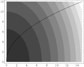
Figure 1: A typical plot of the field trajectory on the two-field potential $V=m_{1}^{2}\phi_{1}^{2}/2+m_{2}^{2}\phi_{2}^{2}/2$ [16]. The horizontal and vertical axes correspond to $\phi_{1}$ and $\phi_{2}$, respectively. Since here we take $m_{1}>m_{2}=0.7m_{1}$, the potential is steeper in the $\phi_{1}$ direction, i.e. the contour lines are denser along $\phi_{1}$ direction, and hence the trajectory is along this direction significantly at the early times. But appreciable $m_{2}$ makes the trajectory “curved” towards the $\phi_{2}$ direction later.

From Eqs. (8) and (9), the slow-roll parameter $\epsilon$ is given by [17]

$$\epsilon=\frac{2m_{\mathrm{Pl}}^{2}\sum_{i}m_{i}^{4}\phi_{i}^{2}}{\left(\sum_{j}m_{j}^{2}\phi_{j}^{2}\right)^{2}}\,.$$ (10)

The other parameters $\eta_{i}$ are, along each direction,

$$\eta_{i}=\frac{2m_{\mathrm{Pl}}^{2}m_{i}^{2}}{\sum_{j}m_{j}^{2}\phi_{j}^{2}}\,.$$ (11)

First consider the simplest case where all the masses are the same. Then, Eq. (7) enjoys perfect rotational symmetry, and this makes every direction physically indistinguishable and thus becomes practically single field inflation. Hence we can set the field trajectory a straight line along one direction, say $\phi_{I}$, with the other orthogonal fields zero [17, 18]. Then we find

$$\epsilon=\eta_{i}=\frac{2m_{\mathrm{Pl}}^{2}}{\phi_{I}^{2}}\,,$$ (12)

so that for the orthogonal fields the spectral index of the field fluctuations, given by Eq. (4), is almost exactly scale invariant. This is an interesting but extremely simple limit: generally we should expect that during inflation the field follows a curved trajectory due to unequal masses.

Now let us break this symmetry in the next simplest two-field case with $m_{1}>m_{2}$ as shown in Fig. 1. Note that the field trajectory along any of these axes will be a straight line. Thus the two directions $\phi_{1}$ and $\phi_{2}$ give the extrema of the curvature of the potential, with along $\phi_{1}$ ($\phi_{2}$) corresponding to the maximum (minimum). Now let us assume that the field trajectory is a straight line on the $\phi_{1}$ axis ($\phi_{2}=0$). Then, the orthogonal direction to the field trajectory is the $\phi_{2}$ direction, and correspondingly

$$\eta_{\sigma}=\eta_{2}=\frac{2m_{\mathrm{Pl}}^{2}m_{2}^{2}}{m_{1}^{2}\phi_{1}^{2}}=\epsilon\frac{m_{2}^{2}}{m_{1}^{2}}\,,$$ (13)

and

$$\eta_{\phi}=\eta_{1}=\epsilon=\frac{2m_{\mathrm{Pl}}^{2}}{\phi_{1}^{2}}\,.$$ (14)

If the orthogonal fluctuations, currently $\phi_{2}$, are responsible for the curvature perturbation we can observe now, then the spectral index, given by Eq. (4), should be negative, i.e. $\eta_{\sigma}/\epsilon<1$. We can easily see

$$\frac{\eta_{\sigma}}{\epsilon}=\frac{\eta_{2}}{\epsilon}=\frac{m_{2}^{2}}{m_{1}^{2}}<1\,,$$ (15)

and indeed in this case the orthogonal field, $\phi_{2}$, may give dominant contribution to the curvature perturbation with right spectral tilt due to post-inflationary dynamics. Note that from Eqs. (4) and (15) to match the observations, we need

$$\epsilon\approx\frac{0.025}{1-m_{2}^{2}/m_{1}^{2}}\,.$$ (16)

When the masses are not equal, $\epsilon$ becomes greater compared with that of the equal mass case and it is unclear by how much it grows without the detail of the model under consideration [17]: from Eq. (7), we can find the number of $e$-folds as

$$\mathcal{N}\equiv\int Hdt=\frac{\sum_{i}\phi_{i}^{2}}{4m_{\mathrm{Pl}}^{2}}\,,$$ (17)

where we have neglected $\mathcal{O}(1)$ constant. For the equal mass case, it is equivalent to the single field chaotic inflation. Thus in terms of $\mathcal{N}$, we can estimate

$$\epsilon>\epsilon_{\mathrm{eq}}=\frac{1}{2\mathcal{N}}\,.$$ (18)

It may be noticed that Eq. (15) is valid for a special case and is not applicable in general. However, this can be easily resolved as long as there are enough number of fields. From Eqs. (10) and (11), the ratio is written as

$$\frac{\eta_{i}}{\epsilon}=\frac{m_{i}^{2}\sum_{j}m_{j}^{2}\phi_{j}^{2}}{\sum_{k}m_{k}^{4}\phi_{k}^{2}}\,.$$ (19)

Exactly for how many fields this ratio is less than one would depend on the underlying mass distribution [11]: for example, as the simplest possibility assume that the masses are randomly distributed over a range. Then, it is easy to expect that roughly half of the fields satisfy the condition $\eta_{i}/\epsilon<1$. More importantly, about 50 $\sim$ 60 $e$-folds before the end of inflation, the field trajectory is almost orthogonal to the most light fields. Thus, the corresponding $\eta_{i}$ of these field fluctuations receive contributions mostly from $m_{i}$ and the effects by other fields, especially those which provide the most significant curvature in the field space at that time, are negligible. However, we stress again that unlike the curvaton type fields the later stage of inflation is driven by these fields and they are indeed the ‘inflaton’ fields.

Finally, let us briefly examine if this is really the case, what would be the distinctive observational signatures from the case where the curvature perturbation is mostly due to the inflaton fluctuations, regarding near future cosmological observations in particular: non-Gaussianity and the tensor-to-scalar ratio. Denoting $\mathcal{N}_{,i}\equiv\partial\mathcal{N}/\partial\phi_{i}$ and $\mathcal{N}_{,ij}\equiv\partial^{2}\mathcal{N}/\partial\phi_{i}\partial\phi_{j}$ and using Eq. (17), the non-linear parameter $f_{\mathrm{NL}}$ is given by [19]

$$-\frac{3}{5}f_{\mathrm{NL}}\approx\frac{\sum_{i,j}\mathcal{N}_{,i}\mathcal{N}_{,ij}\mathcal{N}_{,j}}{2\left(\sum_{k}\mathcal{N}_{,k}^{\,\,2}\right)^{2}}=\frac{m_{\mathrm{Pl}}^{2}}{\sum_{i}\phi_{i}^{2}}=\frac{1}{4\mathcal{N}}\,,$$ (20)

which is far less than 1 and is absolutely not observable as long as relevant non-Gaussian contribution is generated during inflation. However, it is indeed possible that significant non-Gaussianity is obtained by the post-inflationary dynamics: e.g. if the curvaton mechanism is relevant [12, 20],

$$f_{\mathrm{NL}}\sim\frac{5}{4r}\,,$$ (21)

i.e. a small fraction of such fields would give rise to large non-Gaussianity, along with considerable isocurvature perturbation between radiation and matter [21]. It seems impossible to make any completely general and model independent prediction on the level of non-Gaussianity. Meanwhile, the well known result for the tensor-to-scalar ratio, $r=16\epsilon$, gives the ratio of the tensor perturbations to the scalar perturbations due to the inflaton contribution only. In the cases of our interest, however, for the scalar perturbations there exist contributions other than the inflaton component. Thus we can write [22]

$$r=\frac{\mathcal{P}_{\mathrm{T}}}{\mathcal{P}_{\mathrm{s}}}=16\epsilon\frac{\mathcal{P}_{\phi}}{\mathcal{P}_{\phi}+\mathcal{P}_{\sigma}}\,,$$ (22)

which is always smaller than $16\epsilon$, and can be absolutely negligible if the inflaton contribution is sub-dominant.

In summary, we have explored the possibility that during multi-field inflation the spectral indices of the fluctuations of the isocurvature components of the inflaton field are negative. Indeed, at least for some of them the indices are negative and may match the observed value. Therefore as far as the spectral index is concerned, they can be plausible candidates for curvaton type mechanism, and may serve as the dominant contributions to the curvature perturbation relevant for our observable universe, depending on the post-inflationary dynamics. This suggests that the generation of the curvature perturbation in multi-field inflation models is a much more generic phenomenon than usually perceived, and that the studies on this topic should be very careful. Concerned with near future observations, compared with the case where the inflaton contribution is dominant, we cannot make any model independent prediction on non-Gaussianity. The tensor-to-scalar ratio, however, will be smaller and may not be detected in any foreseeable observations.

References

- [1] A. H. Guth, Phys. Rev. D 23, 347 (1981) ; A. D. Linde, Phys. Lett. B 108, 389 (1982) ; A. Albrecht and P. J. Steinhardt, Phys. Rev. Lett. 48, 1220 (1982)
- [2] V. F. Mukhanov and G. V. Chibisov, JETP Lett. 33, 532 (1981) ; S. W. Hawking, Phys. Lett. B 115, 295 (1982) ; A. A. Starobinsky, Phys. Lett. B 117, 175 (1982) ; A. H. Guth and S.-Y. Pi, Phys. Rev. Lett. 49, 1110 (1982) ; J. M. Bardeen, P. J. Steinhardt and M. S. Turner, Phys. Rev. D 28, 679 (1983) ; M. Sasaki, Prog. Theor. Phys. 70, 394 (1983)
- [3] E. D. Stewart and J.-O. Gong, Phys. Lett. B 510, 1 (2001) astro-ph/0101225 ; J. Choe, J.-O. Gong and E. D. Stewart, J. Cosmol. Astropart. Phys. 07, 012 (2004) hep-ph/0405155
- [4] See, e.g. P. Langacker, Phys. Rept. 72, 185 (1981) ; H. P. Nilles, Phys. Rept. 110, 1 (1984)
- [5] See, e.g. D. H. Lyth and A. Riotto, Phys. Rept. 314, 1 (1999) hep-ph/9807278
- [6] A. A. Starobinsky, JETP Lett. 42, 152 (1985) ; M. Sasaki and E. D. Stewart, Prog. Theor. Phys. 95, 71 (1996) astro-ph/9507001 ; M. Sasaki and T. Tanaka, Prog. Theor. Phys. 99, 763 (1998) gr-qc/9801017 ; J.-O. Gong and E. D. Stewart, Phys. Lett. B 538, 213 (2002) astro-ph/0202098 ; D. H. Lyth, K. A. Malik and M. Sasaki, J. Cosmol. Astropart. Phys. 05, 004 (2005) astro-ph/0411220
- [7] A. Linde and V. Mukhanov, Phys. Rev. D 56, R535 (1997) astro-ph/9610219 ; D. H. Lyth and D. Wands, Phys. Lett. B 524, 5 (2002) hep-ph/0110002 ; T. Moroi and T. Takahashi, Phys. Lett. B 522, 215 (2001) hep-ph/0110096 ; Erratum-ibid. B 539, 303 (2002)
- [8] G. Dvali, A. Gruzinov and M. Zaldarriaga, Phys. Rev. D 69, 023505 (2004) astro-ph/0303591 ; G. Dvali, A. Gruzinov and M. Zaldarriaga, Phys. Rev. D 69, 083505 (2004) astro-ph/0305548
- [9] D. N. Spergel et al., astro-ph/0603449
- [10] See, e.g. A. R. Liddle and D. H. Lyth, Cosmological inflation and large scale structure, Cambridge University Press (2000) ; V. F. Mukhanov, Physical foundations of cosmology, Cambridge University Press (2005)
- [11] J.-O. Gong, Phys. Rev. D 75, 043502 (2007) hep-th/0611293
- [12] D. H. Lyth, C. Ungarelli and D. Wands, Phys. Rev. D 67, 023503 (2003) astro-ph/0208055
- [13] D. H. Lyth, Phys. Lett. B 579, 239 (2004) hep-th/0308110 ; J.-O. Gong, Phys. Lett. B 637, 149 (2006) hep-ph/0602106
- [14] S. Dimopoulos, S. Kachru, J. McGreevy and J. G. Wacker, hep-th/0507205
- [15] N. Bartolo and A. R. Liddle, Phys. Rev. D 65, 121301 (2002) astro-ph/0203076
- [16] D. Polarski and A. A. Starobinsky, Nucl. Phys. B 385, 623 (1992) ; D. Langlois, Phys. Rev. D 59, 123512 (1999) astro-ph/9906080
- [17] L. Alabidi and D. H. Lyth, J. Cosmol. Astropart. Phys. 05, 016 (2006) astro-ph/0510441
- [18] C. T. Byrnes and D. Wands, Phys. Rev. D 73, 063509 (2006) astro-ph/0512195
- [19] D. H. Lyth and Y. Rodríguez, Phys. Rev. Lett. 95, 121302 (2005) astro-ph/0504045 ; D. H. Lyth, J. Cosmol. Astropart. Phys. 06, 015 (2006) astro-ph/0602285 ; S. A. Kim and A. R. Liddle, Phys. Rev. D 74, 063522 (2006) astro-ph/0608186
- [20] M. Sasaki, J. Väliviita and D. Wands, Phys. Rev. D 74, 103003 (2006) astro-ph/0607627
- [21] K.-Y. Choi and J.-O. Gong, J. Cosmol. Astropart. Phys. 06, 007 (2007) arXiv:0704.2939 [astro-ph]
- [22] D. H. Lyth, J. Cosmol. Astropart. Phys. 11, 006 (2005) astro-ph/0510443