Breathers and Raman scattering in a two-leg ladder with staggered Dzialoshinskii-Moriya interaction

Abstract

Recent experiments have revealed the role of staggered Dzialoshinskii-Moriya interaction in the magnetized phase of an antiferromagnetic spin 1/2 two-leg ladder compound under a uniform magnetic field. We derive a low energy effective field theory describing a magnetized two-leg ladder with a weak staggered Dzialoshinskii-Moriya interaction. This theory predicts the persistence of the spin gap in the magnetized phase, in contrast to standard two-leg ladders, and the presence of bound states in the excitation spectrum. Such bound states are observable in Raman scattering measurements. These results are then extended to intermediate Dzialoshinskii-Moriya interaction using Exact Diagonalizations.

Antiferromagnetic systems with spin gaps have been the object of great theoretical and experimental interest for the last two decades. In particular, ladder systemsdagotto_2ch_review ; dagotto_supra_ladder_review have been investigated first theoretically as toy models for high-temperature superconductivityrice_srcuo , and then experimentally.takano_spingap Ladder systems with an even number of legs are known to possess a spin gap, while ladders with an odd number of legs are gapless, a result reminiscent of the one of Haldane for antiferromagnetic spin-S chains.haldane_gap Upon application of a magnetic field, the gap of two-leg ladder systems can be closed, leading to the formation of a Luttinger liquid state.chitra_spinchains_field ; furusaki_dynamical_ladder In such a state, there exists a quasi-long range antiferromagnetic order, and inter-ladder exchange leads, at low enough temperature, to the formation of a Néel state.giamarchi_coupled_ladders Such field induced magnetic ordering is the quasi-one dimensional analogue of magnon Bose condensation.nikuni00_tlcucl3_bec

Recent Nuclear Magnetic Resonance (NMR) experimentsclemancey06_cuhpcl have revealed that the compoundchiari_cuhpcl Cu₂(C₅H₁₂N₂)₂Cl₄ (Copper diazacycloheptane to be abbreviated CuHpCl), originally believed to be a simple spin ladder materialchaboussant_cuhpcl ; chaboussant_nmr_ladder ; chaboussant_mapping , possesses staggered Dzialoshinskii-Moriyadzyalo_interaction ; moryia_asym_int (DM) interactions along the rungs. Although recent Inelastic Neutron Scattering experiments suggest that this material is closer to a three-dimensional coupled dimer system stone02_cuhpcl than to a real ladder, it was shown theoretically (using a ladder description) that including such a spin anisotropy greatly improves the low temperature fits of the magnetization curve miyahara06_dm ; capponi06_ladder_dm and of the anomalous behavior of the specific heat in magnetic field. capponi06_ladder_dm Due to the presence of these interactions, the spin gap persists in the magnetized phase, and a staggered magnetization is present even above the temperature for antiferromagnetic ordering.clemancey06_cuhpcl The outline of the paper is the following. In Sec. I, some basic results on two-leg ladders with staggered DM interactions are recalled. Then, in Sec. II, we develop the field theoretical approach and compute the Raman scattering spectra in the Fleury-Loudon approximationfleury_raman ; moriya_raman . We obtain well defined peaks below a continuum. The predictions of the field theoretical treatment are then compared to Exact Diagonalization (ED) results in Sec. III. The existence of peaks is confirmed, and is shown to persist to intermediate couplings.

I Introduction

The Hamiltonian of the spin 1/2 Heisenberg two-leg ladder reads:

$$H = \sum_{n,p=1,2}\!\!J_{\parallel}\mathbf{S}_{n,p}\cdot\mathbf{S}_{n+1,p}+\sum_{n}J_{\perp}\mathbf{S}_{n,1}\cdot\mathbf{S}_{n,2}$$ (1)

$$-h\sum_{n,p=1,2}S_{n,p}^{z},$$

where $\mathbf{S}_{n,p}$ is a spin 1/2 operator, $J_{\perp},J_{\parallel}>0$ and $h=g\mu_{B}H$. The staggered DM interaction is:

$$H_{DM}=\sum_{n}(-)^{n}\mathbf{D}\cdot(\mathbf{S}_{n,1}\times\mathbf{S}_{n,2})$$ (2)

with $\mathbf{D}=D\hat{y}$.

The point group of the Hamiltonian Eqs. (1)– (2) is $C_{2v}$.miyahara06_dm It includes the identity, the reflection symmetry w.r.t. a rung (or “parity”), the inversion symmetry w.r.t the center of a plaquette and the combined operation of the two last ones. The Hamiltonian (1)–(2) is also invariant under translation of two lattice spacing $n\to n+2$.

II Bosonization study

We will derive a weak coupling low-energy theory applying bosonization techniquesgiamarchi_book_1d ; gogolin_1dbook ; nagaosa_book_sc valid for weak rung couplings. Then, in Sec. II.2, we will consider the opposite limit of strong rung exchange and derive an effective spin chain Hamiltonian.chaboussant_mapping ; mila_field By bosonizing the effective spin chain Hamiltonian in the limit of weak DM interaction, we will show that the low energy theory derived for weak rung couplings can be extended to strong rung exchange. In Sec. II.3, we analyze the effective field theory, and show that it supports breather type excitations, in analogy with spin chains with staggered DM interactions along the chains.oshikawa_cu_benzoate_short ; oshikawa_cu_benzoate

II.1 Weak coupling case

In this section, we derive an effective field theory describing the low-energy, long-wavelength excitations of the Hamiltonian Eq. (1)– (2), valid in the limit $J_{\perp},D\ll J_{\parallel}$. The bosonized representation of the Hamiltonian (1) has been derived for $J_{\perp}\ll J_{\parallel}$ in Refs. strong_spinchains, ; strong_spinchains_long, ; shelton_spin_ladders, ; orignac_2spinchains, ; chitra_spinchains_field, . We follow the notations of Ref. orignac_2spinchains, . Using the bosonized representation for the spin operators ($p=1,2$):

$$S_{p}^{+}(x) = \frac{e^{-\imath\theta_{p}(x)}}{\sqrt{2\pi a}}\left[e^{-\imath\frac{\pi x}{a}}+\cos 2\phi_{p}(x)\right],$$

$$S_{p}^{z}(x) = -\frac{1}{\pi}\partial_{x}\phi_{p}+e^{\imath\frac{\pi x}{a}}\frac{\cos 2\phi_{p}(x)}{\pi a},$$ (3)

where $a$ is a lattice cutoff, and $[\phi_{p}(x),\partial_{x}\theta_{p^{\prime}}(x^{\prime})]=i\pi\delta_{p,p^{\prime}}\delta(x-x^{\prime})$, the Hamiltonian of the two-leg ladder is expressed in terms of the fields $\phi_{a}=\frac{\phi_{1}-\phi_{2}}{\sqrt{2}}$ and $\phi_{s}=\frac{\phi_{1}+\phi_{2}}{\sqrt{2}}$ giving:

$$H = H_{s}+H_{a}$$

$$H_{s} = \int\frac{dx}{2\pi}\left[u_{s}K_{s}(\pi\Pi_{s})^{2}+\frac{u_{s}}{K_{s}}(\partial_{x}\phi_{s})^{2}\right]-\frac{h}{\pi}\int dx\partial_{x}\phi_{s}+\frac{2J_{\perp}a}{(2\pi\alpha)^{2}}\int dx\cos(\sqrt{8}\phi_{s}),$$ (4)

$$H_{a} = \int\frac{dx}{2\pi}\left[u_{a}K_{a}(\pi\Pi_{a})^{2}+\frac{u_{a}}{K_{a}}(\partial_{x}\phi_{a})^{2}\right]+\frac{2J_{\perp}a}{(2\pi\alpha)^{2}}\int dx\cos(\sqrt{8}\phi_{a})+\frac{2J_{\perp}a}{(2\pi\alpha)^{2}}\int dx\cos(\sqrt{2}\theta_{a}),$$

where we have written $\partial_{x}\theta_{p}=\pi\Pi_{p}$. It can be shownstrong_spinchains ; orignac_2spinchains that for $h=0$ the Hamiltonian (4) has gapped excitations, with a gap $\Delta$ of order $J_{\perp}$ and that the fields have the following expectation values $\langle\phi_{s}\rangle=\pi/\sqrt{8}$ and $\langle\theta_{a}\rangle=\pi/\sqrt{2}$. Using (II.1), we find the bosonized form of $H_{DM}$:

$$H_{DM}=D\int dx\left[\frac{1}{\pi\sqrt{2\pi a}}(\partial_{x}\phi_{2}\cos\theta_{1}-\partial_{x}\phi_{1}\cos\theta_{2})-\frac{1}{\pi a\sqrt{2\pi a}}(\cos\theta_{1}-\cos\theta_{2})\cos 2\phi_{1}\cos 2\phi_{2}\right].$$ (5)

In the presence of a nonzero magnetic field the term $-h\int dx\partial_{x}\phi_{s}/\pi$ has non-trivial effects on the spectrum.chitra_spinchains_field For $D=0$, it induces a commensurate-incommensurate transition for $h=\Delta$.japaridze_cic_transition ; pokrovsky_talapov_prl In the commensurate state ($h<\Delta$), the system remains gapped and non magnetized, whereas in the incommensurate phase ($h>\Delta$) it is gapless and has a uniform magnetization $m>0$. If a small $D\neq 0$ is turned on in the incommensurate phase, the existence of a nonzero magnetization allows the substitution $\langle\partial_{x}\phi_{1,2}\rangle\to m$ in Eq. (5) , giving a term $mD(\cos\theta_{1}-\cos\theta_{2})$. Taking into account the fact that, in the incommensurate phase, one still has $\langle\theta_{a}\rangle=\pi/\sqrt{2}$, this term reduces to $mD\langle\sin\theta_{a}/\sqrt{2}\rangle\sin(\theta_{s}/\sqrt{2})$. The gap in the antisymmetric modes is given byorignac_2spinchains : $\Delta_{DM}\sim J_{\parallel}(J_{\perp}/J_{\parallel})^{\frac{2K_{a}}{4K_{a}-1}}$, giving$\langle\sin\theta_{a}/\sqrt{2}\rangle\sim(J_{\perp}/J_{\parallel})^{1/(16K_{a}-4)}$ For a magnetic field not too strong, $K_{a}\simeq 1/2$ so that $\langle\sin\theta_{a}/\sqrt{2}\rangle\sim(J_{\perp}/J_{\parallel})^{1/4}$.

The low energy Hamiltonian describing the behavior of a magnetized two-leg ladder with staggered Dzialoshinskii-Moriya interaction is therefore:

$$H_{s} = \int\frac{dx}{2\pi}\left[u_{s}K_{s}(\pi\Pi_{s})^{2}+\frac{u_{s}}{K_{s}}(\partial_{x}\phi_{s})^{2}\right]$$ (6)

$$+\int dx\frac{Dm\langle\sin(\theta_{a}/\sqrt{2})\rangle}{2\pi}\sin\frac{\theta_{s}}{\sqrt{2}}.$$

Such a description is valid for energy scales much lower than $|h-\Delta|$, and is therefore only applicable in a system which is sufficiently magnetized. Let us briefly discuss its symmetries. It is obvious that the Hamiltonian (6) is invariant under parity and translation by two sites. From (II.1), translation by one lattice site amounts to $\theta_{1,2}\to\theta_{1,2}+\pi$ and $\phi_{1,2}\to\phi_{1,2}+\pi/2-\pi ma$, and interchange of the chains to $\theta_{1}\leftrightarrow\theta_{2}$ and $\phi_{1}\leftrightarrow\phi_{2}$. The combination of these two transformations leaves the Hamiltonian invariant. Such combination amounts to $\theta_{s}\to\theta_{s}+\pi\sqrt{2}$, $\theta_{a}\to-\theta_{a}$ and $\phi_{s}\to\phi_{s}+\pi/\sqrt{2}(1-2ma)$ and $\phi_{a}\to-\phi_{a}$. It is immediately seen that this combined transformation leaves the Hamiltonian (6) invariant. The Hamiltonian (6) is the one of a sine-Gordon model, and its spectrum is massive provided $K_{s}>1/16$. Since in the magnetized phasechitra_spinchains_field $K_{s}\simeq 1/2$, the ladder with staggered DM interaction remains gapped for all $h$, as found in DMRG and ED.miyahara06_dm ; capponi06_ladder_dm The gap is of order $\Delta_{DM}\sim J_{\parallel}(Dm/J_{\parallel})^{8K_{s}/(16K_{s}-1)}\sim J_{\parallel}(mD/J_{\parallel})^{4/7}$. It can be seen from Eq. (II.1) that this implies a staggered magnetization with: $\langle S_{n,1}^{x}\rangle=-\langle S_{n,2}^{x}\rangle\sim J_{\parallel}(Dm/J_{\parallel})^{1/(16K_{s}-1)}\sim J_{\parallel}(mD/J_{\parallel})^{1/7}$. Since the dual field of $\phi_{s}$ is ordered, the correlation functions of the non-uniform magnetization along $z$ present an exponential decay instead of the power law decay obtained for $D=0$.furusaki_dynamical_ladder ; giamarchi_coupled_ladders

II.2 Strong coupling case

In this section, we consider again the two-leg ladder, Eqs. (1)– (2), but this time, we assume a strong coupling limit such that $J_{\perp}\gg J,D$. In that case, it is reasonable to diagonalize first the rung interaction and derive an effective spin chain model to describe the behavior of the system under field.chaboussant_mapping ; mila_ladder_strongcoupling We can write:

$$S_{n,1}^{z}=S_{n,2}^{z} = \frac{1}{4}(1+2\tau_{n}^{z})$$

$$S_{n,1}^{+}=-S_{n,2}^{+} = -\frac{1}{\sqrt{2}}\tau_{n}^{+}$$ (7)

where the pseudospin $\tau_{n}^{z}=-1/2$ when the $n-$th rung is in the singlet state, and $\tau_{n}^{z}=+1/2$ when the $n-$th rung is in the triplet state with $S_{n,1}^{z}+S_{n,2}^{z}=1$. In the absence of the DM interaction, the Hamiltonian of the effective spin 1/2 chain readsmila_ladder_strongcoupling ; giamarchi_coupled_ladders :

$$H = \frac{J_{\parallel}}{2}\sum_{n}(\tau_{n}^{+}\tau_{n+1}^{-}+\tau_{n}^{-}\tau_{n+1}^{+}+\tau_{n}^{z}\tau_{n+1}^{z})$$ (8)

$$- (h-J_{\perp}-J_{\parallel})\sum_{n}\tau_{n}^{z}$$

Deriving a strong coupling expansion for Eq. (2), we find that:

$$H_{DM}=\frac{D}{\sqrt{2}}\sum_{n}(-1)^{n}\tau_{n}^{x}.$$ (9)

Note that substituting simply (II.2) in (2) yields a result which is incorrect by a factor 1/2. The reason for this is that the operators $S_{n,1/2}^{z}$ do not annihilate the singlet state contrarily to their low energy representation in terms of the pseudospins. As a result of this, some of the contributions to (9) are missed if we simply replace in (2) the spin operators by their strong coupling expansion (II.2).

Let us briefly review the symmetries of the strong coupling model. First, we notice that the model is invariant under a translation of two lattice spacing $n\to n+2$. Second, it is also invariant under inversion $n\to-n$. Third, it is also invariant under a reflexion around the middle of a bond $n\to 1-n$ (or a translation of one lattice site) combined with a rotation of $\pi$ around the $z$ axis. If we turn to the two-leg ladder, we notice that that this latter symmetry was apparently not present in the original model. It is in fact the inversion symmetry around the center of a plaquette in disguised form. Under inversion, singlet states change sign (as $|\uparrow_{1}\downarrow_{2}\rangle-|\uparrow_{2}\downarrow_{1}\rangle\to-|\uparrow_{2}\downarrow_{1}\rangle-|\uparrow_{1}\downarrow_{2}\rangle$), but triplet states do not. As a result, operators that transform singlet state into triplet one are odd under inversion, and operators diagonal on singlet or triplet states are even. Thus, in the effective model, inversion becomes the transformation $\tau_{n}^{+}\to-\tau_{1-n}^{+}$ and $\tau_{n}^{z}\to+\tau_{1-n}^{z}$, i. e. a reflection around the middle of a bond combined with a rotation of $\pi$ around the $z$ axis.

Eq. (9) shows that the ladder under strong field with a small staggered Dzialoshinskii-Moriya interaction becomes equivalent to a XXZ spin chain in a staggered magnetic field. In the limit $D\ll J_{\perp}$ , this problem can be treated using bosonizationluther_chaine_xyz ; giamarchi_book_1d , and the amplitude of the perturbation can even be found exactly.lukyanov_ampl_xxz ; lukyanov_spinchain_asymptotics ; lukyanov_xxz_asymptotics Similar results are known to hold in the case of spin 1/2 chains with a longitudinal staggered Dzialoshinskii-Moriya interaction.oshikawa_cu_benzoate ; essler99_cu_benzoate ; essler_benzocu Our bosonized theory reads:

$$H=\!\int\!\frac{dx}{2\pi}\left[uK(\pi\Pi)^{2}\!+\!\frac{u}{K}(\partial_{x}\phi)^{2}\right]\!+\!\frac{\lambda D}{a\sqrt{2}}\int\!\!dx\cos\theta,$$ (10)

where $u$ and $K$ can be obtained from (8) by Bethe Ansatz techniquesgiamarchi_coupled_ladders provided that $D\ll J_{\parallel}$. This is a quantum sine-Gordon (SG) model.coleman_equivalence For $K>1/8$, its spectrum contains massive solitons note_soliton , which means that the original Hamiltonian possesses a spin gap. The magnitude of the gap will be $\Delta_{DM}\propto J_{\parallel}(D/J_{\parallel})^{4K/(8K-1)}$ provided that $K>1/8$. We note that this strong coupling bosonized Hamiltonian is of the same form as the one derived in Sec. II.1, indicating that the weak and the strong coupling regime are continuously connected. The formal correspondence between the two Hamiltonians is obtained by the canonical transformation $\theta=\frac{\pi}{2}-\theta_{s}/\sqrt{2}$, $\phi=-\phi_{s}\sqrt{2}$, $K=2K_{s}$. In terms of the sine-Gordon model (10), the symmetries of the lattice Hamiltonian become continuous translational invariance, invariance under the transformation $\theta(x)\to\theta(-x)$ and $\phi(x)\to-\phi(-x)$ and $\theta\to\theta+\pi$, $D\to-D$. This latter symmetry is a $Z_{2}$ gauge symmetry resulting from the impossibility of discerning odd and even sites in the continuum limit. A final symmetry of the bosonized Hamiltonian is $\theta\to-\theta$ and $\phi\to-\phi$. The latter symmetry is a consequence of the linear dispersion of excitations for $D=0$ in the scaling limit and is absent in the lattice system. From the semiclassical treatmentdashen_sinegordon , it is seen that parity transforms solitons into antisolitons and vice-versa while leaving the breathers invariants. Indeed, classically, the soliton (resp. antisoliton) of the Sine-Gordon model is given by $\theta(x)=4\arctan{(\exp{(x/l)})}$ (resp. $\theta(x)=4\arctan{(\exp{(-x/l)})}$) so that the two are exchanged by a parity transformation. States odd or even under parity can be constructed by linear combination of soliton and antisoliton states. Lastly, we note that the bound states corresponding to the SG breathers should be even under parity as breathers contain an equal number of solitons and antisolitons note_breathers .

An interesting aspect of the Hamiltonian (10) is that it can possess breathers (bound states of solitons) as excited states provided $K>1/4$.solyom_revue_1d ; dashen_sinegordon ; luther_chaine_xyz It can be seen from Ref. giamarchi_coupled_ladders, that this condition is always satisfied. If $M_{0}\propto\Delta_{DM}$ is the mass of a soliton, the masses of the breathers will be given by:

$$M_{n}=2M_{0}\sin\left(\frac{\pi}{2}\frac{n}{8K-1}\right),$$ (11)

with $n$ integer and $1\leq n<8K-1$. Under the transformation $\phi\to-\phi$ and $\theta\to-\theta$ breathers with an odd $n$ are odd, while breathers with an even $n$ are even.

In the case of a spin chain with a longitudinal staggered Dzialoshinskii-Moriya interaction, the effective theory is also a sine-Gordon model as Eq. (10), but with $K=1/2$ for not too large applied magnetic field. This leads to a smaller number of breathers than in the ladder case.asano_breather ; zvyagin05_esr_cu_pyrimidine ; bertaina_bacu2ge2o7_esr ; nojiri_breather Such breathers have been be detected in Electron Spin Resonance (ESR) measurements.asano_breather ; feyerherm_breather ; wolter03_field_gap ; bertaina_bacu2ge2o7_esr ; kenzelmann_breather ; zvyagin_breather ; wolter_canting ; zvyagin05_esr_cu_pyrimidine ; morisaki_dzialmo ; nojiri_breather ; morisaki07_staggered_dm In the case of the ladder system however, ESR measurements cannot be straightforwardly interpreted. Indeed, ESR absorption intensity is proportional to an autocorrelation function of $(S_{1}^{x}+S_{2}^{x})$, but this operator is vanishing in the strong coupling limit according to (II.2) and in the weak coupling limit it is mixing the symmetric and the antisymmetric modes, thus complicating the interpretation of the spectra. We suggest in Sec. II.3 that Raman scattering intensity measurements give a direct access to these breather modes in the ladder systems.

Let us now discuss the variation of the number of breathers with the magnetization in the case of the ladder. For a magnetization near zero, we have $K\lesssim 1$ so we expect to find 6 breather excitations with masses given by (11). As the magnetization increases, $K$ decreases, and for $K<7/8$ there will be only 5 breathers. When $K=3/4$, i.e. at half the saturation magnetization, there are only 4 breathers. As the magnetization increases beyond this value, $K$ becomes an increasing function of the magnetization, and the number of breathers becomes again increasing.

When the magnetization is at half the saturation value, a more quantitative analysis of the gap becomes possible. Indeed, in that case $\langle\tau_{n}^{z}\rangle=0$ and the exponent $K$ and the velocity $u$ are given as:luther_chaine_xxz ; haldane_xxzchain

$$K = 3/4,$$ (12)

$$u = \frac{3\sqrt{3}}{8}J_{\parallel}a.$$

Moreover, the amplitude $\lambda$ is given by the integral:lukyanov_ampl_xxz ; lukyanov_xxz_asymptotics ; hikihara03_amplitude_xxz

$$\lambda^{2}=\frac{1}{4\left(1-\frac{1}{2K}\right)^{2}}\left[\frac{\Gamma\left(\frac{1/2}{2K-1}\right)}{2\sqrt{\pi}\Gamma\left(\frac{K}{2K-1}\right)}\right]^{\frac{1}{2K}}\exp\left[-\int_{0}^{\infty}\frac{dt}{t}\left(\frac{\sinh\left(\frac{t}{2K}\right)}{\sinh t\cosh\left[\left(1-\frac{1}{2K}\right)t\right]}-\frac{e^{-2t}}{2K}\right)\right],$$ (13)

which can be evaluated using Ref. abramowitz_math_functions, , Eq. (6.3.22) giving:

$$\lambda^{2}=\frac{9}{4\pi^{2/3}}\left(\frac{\Gamma(2/3)}{\Gamma(1/3)}\right)^{2}.$$ (14)

This expression yields $\lambda\simeq 0.51769$ in agreement with Table I in Ref. hikihara03_amplitude_xxz, . Finally, using the expression of the gap of the sine Gordon model from Ref. lukyanov_sinegordon_correlations, , we obtain the quantitative expression of the spin gap:

$$\frac{\Delta_{DM}}{J_{\parallel}}=\frac{3\sqrt{3}}{4\sqrt{\pi}}\frac{\Gamma(1/10)}{\Gamma(3/5)}\left(\frac{\pi^{2/3}\Gamma(5/6)\Gamma(2/3)}{\Gamma(1/6)\Gamma(1/3)}\sqrt{\frac{2}{3}}\frac{D}{J_{\parallel}}\right)^{3/5}$$ (15)

i.e. $\Delta_{DM}/J_{\parallel}\simeq 1.67(D/J_{\parallel})^{3/5}$. Inserting the result (12) in Eq. (11) leads to the prediction of four breathers with energies $E_{n}=2\Delta_{DM}\sin(n\pi/10)$ ($n=1,\ldots,4$). We notice that the energy of the lowest breather is smaller than the energy of the soliton. If we assume that the spin gap coincides with the energy of the lowest breather mode, we will find a spin gap $E_{1}=1.032J_{\parallel}(D/J_{\parallel})^{3/5}$. This formula is in rough agreement with the numerical data of Sec. III. To obtain quantitative estimates of the spin gap away from half the saturation magnetization, where (13) is not applicable anymore, one can use the numerical estimations of the amplitude $\lambda$ obtained in Ref. hikihara03_amplitude_xxz, . This will not be attempted here.

II.3 Raman scattering intensity

In that section, we determine the Raman scattering intensity of the two-leg ladder under a magnetic field in the limit $D,J_{\parallel}\ll J_{\perp}$. We will assume that the Fleury-Loudon approximationfleury_raman ; moriya_raman is applicable, i.e. that the frequency of the radiation is much smaller than the Mott gap of the material.shastry_raman In that case, the (effective) Raman operator acts in the (restricted) Hilbert space of the spin configurations and can be written as:

$$\hat{O}_{R}=\sum_{\langle ij\rangle}J_{ij}(\hat{e}_{I}\cdot\hat{n}_{ij})(\hat{e}_{O}\cdot\hat{n}_{ij}){\bf S}_{i}\cdot{\bf S}_{j}$$ (16)

where the $\hat{n}_{ij}$ are unit vectors along the bond directions, $\hat{e}_{I}$ the polarization vector of incoming light, and $\hat{e}_{O}$ the polarization vector of outgoing light. In principle, the strength of the Raman scattering $J_{ij}$ could depend on the geometry freitas_raman but, as in most studies natsume_ladder_raman , we assume it to be constant.

For simplicity, here we restrict ourselves to simple geometrical setups, e.g. to the XX, YY and X’Y’ geometries corresponding to $\hat{e}_{I}$ and $\hat{e}_{O}$, both along the chains direction, both perpendicular to the chains and at 45-degrees from the crystal axes (X’=X+Y, Y’=X-Y), respectively. The corresponding Raman operators can then be written as,

$$\hat{O}_{R}^{XX} = \gamma\sum_{n}({\bf S}_{n,1}\cdot{\bf S}_{n+1,1}+{\bf S}_{n,2}\cdot{\bf S}_{n+1,2})\,,$$ (17)

$$\hat{O}_{R}^{YY} = \gamma\sum_{n}{\bf S}_{n,1}\cdot{\bf S}_{n,2}\,,$$ (18)

$$\hat{O}_{R}^{X^{\prime}Y^{\prime}} = \frac{1}{2}(\hat{O}_{R}^{XX}-\hat{O}_{R}^{YY})\,.$$ (19)

In the absence of DM interaction, it is expected that there is no Raman intensity for frequencies smaller than twice the spin gap.orignac_raman_short ; bibikov_raman_ladder ; donkov_raman_ladder ; natsume_ladder_raman For frequencies equal to approximately twice the spin gap, a threshold is obtained when interaction between magnons are neglectedorignac_raman_short ; bibikov_raman_ladder with the Raman intensity behaving as $I_{R}(\omega)\sim(\omega-2\Delta)^{1/2}$. When interactions are added, the threshold becomes a peak.donkov_raman_ladder Turning to the ladder with Dzialoshinskii-Moriya interaction, in the weak coupling case, the threshold at twice the spin gap will be obtained from the contribution of antisymmetric modes $\theta_{a}/\phi_{a}$ to the Raman intensity.orignac_raman_short The symmetric modes will give extra peaks and thresholds but at energy scales small compared to the gap. In the following, we will compute the Raman intensity for frequencies smaller than $2J_{\perp}$. In that case, we can use the strong coupling theory for the calculation. We will consider two cases, that of a field parallel to the legs in Sec. II.3.1, and then that of a field parallel to the rungs in Sec. II.3.2.

II.3.1 Electric field along the legs

In the strong coupling limit, we can use Eq. (II.2) to rewrite the Raman operator (17) as,

$$\hat{O}_{R}^{XX} = \frac{\gamma}{2}\sum_{n}(\tau_{n}^{+}\tau_{n+1}^{-}+\tau_{n+1}^{+}\tau_{n}^{-}$$ (20)

$$+ (\tau_{n}^{z}+1/2)(\tau_{n+1}^{z}+1/2)),$$

yielding the expression:

$$\hat{O}_{R}^{XX}=\gamma\frac{H-H_{DM}+(h-J_{\perp}-J_{\parallel}/2)\sum\tau_{n}^{z}}{J_{\parallel}}+\text{const.},$$ (21)

where $H$ is the full strong coupling effective spin chain Hamiltonian. In the computation of the Raman scattering intensityorignac_raman_short , we had already noticed that the time independent terms would drop out from the calculation. Therefore, we can consider the effective Raman operator:

$$\hat{O}_{R}^{XX}=\gamma(h_{0}\sum_{n}\tau_{n}^{z}-H_{DM})/J_{\parallel},$$ (22)

where $h_{\text{0}}=h-J_{\perp}-J_{\parallel}/2$. Going to the continuum limit, it is convenient to introduce a density for the Raman operator, $O^{XX}_{R}(x)$ so that $\hat{O}_{R}^{XX}=\int O_{R}^{XX}(x)dx$. Using the density of Raman operator, and the standard definition of Raman scattering intensity, we finally find that:

$$I_{R,\parallel}(\omega)=\sum_{n}|\langle n,\mathbf{P}_{n}=0|O^{XX}_{R}(0)|0\rangle|^{2}\delta(\omega-E_{n})$$ (23)

where $|0\rangle$ is the ground state (GS) of the system and $|n,\mathbf{P}_{n}\rangle$ is the $n-$th excited state with $\mathbf{P}_{n}$ its total momentum. The Raman operator being given by a sum over all sites, it is easy to show by Fourier transformation that Raman scattering is conserving photon momenta. This explains why only the states with zero momenta (i.e. having the same momentum as the ground state) contribute to the sum.

To proceed with the calculation, we need the bosonized expression of the density of Raman operator. It is easy to show that it reads:

$$O^{XX}_{R}(x)=\frac{\gamma}{J_{\parallel}}\left(\frac{\lambda D}{a\sqrt{2}}\cos\theta(x)-\frac{h_{0}}{\pi}\partial_{x}\phi\right)$$ (24)

The Raman intensity can now be found by applying the Form Factor methodkarowski_ff ; mussardo_trieste_2001 ; controzzi_mott . The form factors of an operator are simply the matrix elements of this operator between the ground state and an excited state. In the sine-Gordon model, the excited states are formed of solitons, antisolitons and breathers with given rapidities. Because in one dimensional integrable models collisions between particles do not lead to production of new particlesdorey_smatrix_review , the form factors are derived from the sole knowledge of the exact S-matrices of the sine-Gordon model.zamolodchikov79_smatrices ; dorey_smatrix_review ; mussardo_offcritical_review

In our case, the relevant form factors have been already computed by other authors in slightly different contextscontrozzi_mott ; essler98_cu_benzoate . Using the symmetries of the operators in Eq. (24), it is possible to further simplify the expression of the Raman intensity. The sine-Gordon Hamiltonian is invariant under the simultaneous transformations $\theta\to-\theta$ and $\phi\to-\phi$, and its eigenstates can be classified according to their parity under this transformation. We note that the operator $\cos\theta$ is even under such transformation, whereas the operator $\partial_{x}\phi$ is odd. Therefore, the non-vanishing matrix elements of $\cos\theta$ are between the ground state and even states, whereas those of $\partial_{x}\phi$ are between the ground state and the odd states. An immediate consequence is that:

$$I_{R,\parallel}(\omega)=I_{R,\parallel}^{(o)}(\omega)+I_{R,\parallel}^{(e)}(\omega),$$ (25)

where:

$$I_{R,\parallel}^{(o)}(\omega) = \left(\frac{\gamma h_{0}}{\pi J_{\parallel}}\right)^{2}\sum_{|n\rangle odd}|\langle n|\partial_{x}\phi|0\rangle|^{2}\delta(\omega-E_{n})$$ (26)

$$I_{R,\parallel}^{(e)}(\omega) = \left(\frac{\lambda\gamma D}{aJ_{\parallel}\sqrt{2}}\right)^{2}\sum_{|n\rangle even}|\langle n|\cos\theta|0\rangle|^{2}\delta(\omega-E_{n})$$

The intensity $I_{R,\parallel}^{(e)}(\omega)$ has been computed previously in Ref. essler98_cu_benzoate in the context of spin chains with staggered Dzialoshinskii-Moriya interactions. ¿From the results of Ref. essler98_cu_benzoate, , $I_{R,\parallel}^{(e)}(\omega)$ contains delta-function peaks at the frequencies of even breathers, and thresholds at frequencies equal to twice the soliton frequency, and to frequencies equal to the sum of the masses of two breathers of identical parity. The lowest threshold is therefore obtained at the frequency $\omega=2M_{1}$. We notice that this threshold is below the energies of the breathers of mass $M_{3}$ and $M_{4}$. Therefore, peaks are obtained in the continuum. Of course, in a more realistic model, the conservation laws that make the sine Gordon model integrable would be absent, and one should expect that the peaks would be broadened by coupling with the continuum. If the deviations of the lattice model from the continuum sine-Gordon model are sufficiently important (for instance if the gap is so large that the continuum limit is not justified), they may even lead to the complete disappearance of the two peaks.

Turning to the intensity $I_{R,\parallel}^{(o)}(\omega)$, we use the equation of motion for the field $\theta$, $\partial_{t}\theta=\frac{u}{K}\partial_{x}\phi$, to relate it to the electrical conductivity of a one dimensional Mott insulator.controzzi_mott ; essler_mott_excitons1d In Ref. essler_mott_excitons1d, , it was shown that if the sine-Gordon model describing the low energy charge excitations of the Mott insulator possesses breathers in its spectrum, the conductivity of the Mott insulator has delta peaks at the breather frequencies. In the context of the Mott insulator, these peaks were interpreted as exciton lines.essler_mott_excitons1d Translating the results of Ref. essler_mott_excitons1d, , we conclude immediately that $I_{R,\parallel}^{(o)}(\omega)$ possesses delta function peaks at the frequencies of the odd breathers. Moreover, there are thresholds at frequencies equal to twice the soliton mass and to the sum of two breather masses of different parities. The first threshold in $I_{R,\parallel}^{(o)}(\omega)$ is thus at the frequency $\omega=M_{1}+M_{2}$.

Combining the two contributions, both the odd and the even breathers yield peaks in the Raman intensity. Moreover, the Raman intensity exhibits thresholds at all frequencies equal to the sum of two breather masses or to twice the soliton mass. A qualitative sketch of the Raman intensity is visible on the figure 1.

Figure 1: A sketch of the Raman intensity for polarization parallel to the legs. The arrows represent the position of the the breathers $\delta$–peaks. The intensity in the peak, proportional to its height is decreasing with the breather index. The continuum starts at a frequency equal to twice the mass of the lightest breather. Above the threshold, resonances are expected instead of $\delta$-functions (beyond a SG analysis).

In the special case of $h_{\text{eff}}=0$, the intensity $I_{R,\parallel}^{(o)}$ is vanishing. Only the even breathers will contribute to the Raman spectrum.

The weight of the delta peaks can be computed by the Form factor expansion.babujian99_ff_sg_1 ; babujian02_ff_sg_2 ; lukyanov97_ff_sinegordon From the general form factor expansion, we have that:

$$I_{R}(\omega)=\sum_{n}|\langle 0|\hat{O}_{R}|B_{n}(0)\rangle|^{2}\frac{\delta(\omega-E_{n})}{E_{n}},$$ (27)

where $|B_{n}(0)\rangle$ is the state with one $B_{n}$ breather of momentum zero, $E_{n}$ the energy of the breather and $\langle 0|\hat{O}_{R}|B_{n}(0)\rangle$ is the one breather form factor. Note that this formula a priori applies to both $\parallel$ or $\perp$ setups corresponding to the XX and YY (see below) polarizations.

Our task is thus to compute the one breather form factors for the two operators $\partial_{t}\theta$ and $\cos\theta$. Let us first sketch the idea behind the calculation. The axioms of Form-Factor theory state that the existence of breathers result in poles in the $n$-particle form-factor (considered as complex function of the rapidities of the particles) when the difference of two rapidities is equal to a (purely imaginary) fusion angle.mussardo_offcritical_review ; smirnov92_ff_book The residue at the pole is proportional to the $(n-2)$ particle, one bound state form-factor. Therefore, the Form-factor for a single soliton bound-state will be obtained from the residue of the two particle form factor at the appropriate fusion angle.

To be more precise, in the case of the sine-Gordon model, one has for the soliton-antisoliton form factor of an operator $O$:

$$F^{O}(\theta)_{\theta\to iu}=\frac{R}{\theta-iu}+\ldots$$ (28)

where:

$$R=\langle 0|O|B\rangle\frac{(-)^{k}i}{\sqrt{2}}\left|\mathrm{Res}S(\theta)\right|^{1/2},$$ (29)

with $=\langle 0|O|B\rangle$ the form factor of the breather, $u$ the corresponding fusion angle, and $S$ the $S-$matrix for soliton-antisoliton collision in the sine-Gordon model. In the case of the sine-Gordon modelbabujian02_ff_sg_2 , the $k-$th fusion angle is given by $u=\pi(1-k/\lambda)$, with $\lambda=8K-1$. The residue of the $S$-matrix is given by:

$$\left|\mathrm{Res}S(\theta)\right|_{\theta=i\pi(1-k/\lambda)}=2\cot\left(\frac{\pi k}{2\lambda}\right)\prod_{\ell=1}^{k-1}\cot^{2}\left(\frac{\pi\ell}{2\lambda}\right)$$ (30)

The soliton-antisoliton form-factor for $\partial_{t}\theta$ is given by:

$$\langle 0|\partial_{t}\theta|\varphi_{1},\varphi_{2}\rangle = \frac{4M}{\beta}\cos\!\left(\!\frac{\varphi_{1}+\varphi_{2}}{2}\!\right)$$ (31)

$$\frac{\cosh\frac{1}{2}(i\pi-\varphi)}{\cosh\frac{\lambda}{2}(i\pi-\varphi)}F_{min}(\varphi),$$

where $\varphi=\varphi_{1}-\varphi_{2}$, And the one of $e^{i\theta}$ by:

$$\langle 0|e^{i\theta}|\varphi_{1},\varphi_{2}\rangle=\frac{\cosh(\varphi/2)e^{\lambda(i\pi-\varphi)/2}}{\sinh\lambda({i\pi-\varphi})}F_{min}(\varphi),$$ (32)

Where:

$$F_{min}(\varphi) = \exp\left[\int_{0}^{\infty}\frac{dt}{t}\frac{\sinh\frac{t}{2}\left(1-\frac{1}{\lambda}\right)}{\cosh\frac{t}{2}\sinh\left(\frac{t}{2\lambda}\right)}\right.$$ (33)

$$\left.\frac{\sin^{2}\frac{t}{2\pi}(\pi-i\varphi)}{\sinh t}\right]$$

As a function of the fusion angle, the energy of the breather is $2M\cos(u/2)=2M\sin(k\pi/2\lambda)$. The Form factor of $\partial_{t}\theta$ has poles only for odd $n$ whereas the Form factor of $e^{i\theta}$ has poles for both odd and even $k$. Hovever, the poles at odd $k$ are the contribution of $\sin\theta$ and therefore, only the poles for even $k$ must be considered in order to obtain the contribution of the $\cos\theta$ term to the Raman intensity. We find:

$$|\langle 0|\partial_{t}\theta|B_{2n+1}(0)\rangle|^{2}=C_{1}\sin\left(\frac{\pi(2n+1)}{\lambda}\right)\prod_{\ell=1}^{2n}\tan^{2}\left(\frac{\pi\ell}{2\lambda}\right)\exp\left[-2\int_{0}^{\infty}\frac{dt}{t}\frac{\sinh\frac{t}{2}\left(1-\frac{1}{\lambda}\right)}{\cosh\frac{t}{2}\sinh\left(\frac{t}{2\lambda}\right)}\frac{\sinh^{2}\left(\frac{(2n+1)t}{2\lambda}\right)}{\sinh t}\right],$$ (34)

recovering the result in Ref. essler_mott_excitons1d, , and:

$$|\langle 0|\cos\theta|B_{2n}(0)\rangle|^{2}=C_{2}\sin^{2}\left(\frac{2\pi n}{\lambda}\right)\tan\left(\frac{\pi n}{\lambda}\right)\prod_{\ell=1}^{2n-1}\tan^{2}\left(\frac{\pi\ell}{2\lambda}\right)\exp\left[-2\int_{0}^{\infty}\frac{dt}{t}\frac{\sinh\frac{t}{2}\left(1-\frac{1}{\lambda}\right)}{\cosh\frac{t}{2}\sinh\left(\frac{t}{2\lambda}\right)}\frac{\sinh^{2}\left(\frac{2nt}{2\lambda}\right)}{\sinh t}\right],$$ (35)

where $C_{1}$ and $C_{2}$ are independent of $n$. In the case of $K=3/4$, we have 4 breathers. The weight of the peak associated with the first breather is obtained numerically as $0.345C_{1}$. For the peak associated with the third breather the weight is only $0.0116C_{1}$ i.e. about 3% of the weight of the first breather. Similarly, the weight of the second breather, we is $0.0367C_{2}$ and the weight of the fourth breather is $0.0058C_{2}$ i. e. about 16% of the intensity associated of the second breather. Note that the ratio $C_{2}/C_{1}$ depends not only on the Luttinger parameter but also on the ratio $D/J_{\parallel}$.

II.3.2 Electric field along the rungs

In the case of an electric field parallel to the rungs, the Raman operator (18) can be rewritten, in the strong coupling limit, as:

$$\hat{O}^{YY}_{R}=\gamma\sum_{n}\left(\tau_{n}-\frac{1}{4}\right)\,.$$ (36)

In the absence of the Dzialoshinskii-Moriya interaction, this term is proportional to the total magnetization, which leads to a vanishing Raman intensity for $\omega\neq 0$. However, this result is only valid for frequencies $\omega\ll J_{\perp}$ since the strong coupling approximation eliminates the states $S^{z}=0,1$ that are placed at energies $\sim J_{\perp}$ above the triplet and the singlet. From the results of Ref. orignac_raman_short, , we know that for $\omega$ equal to twice the spin gap, a photon can create a pair of magnons, resulting in a non-zero Raman intensity. Therefore, in a two-leg ladder with $D=0$ the Raman intensity should be zero in an interval $[0,2(J_{\perp}-J_{\parallel})]$.

When we turn on $D$, the total magnetization is not anymore a good quantum number, and we expect a non-zero Raman intensity also for energies small compared to $J_{\perp}$. Using bosonization, we can express the Raman intensity as:

$$I_{R,\perp}(\omega)=\frac{K^{2}\gamma^{2}}{\pi^{2}u^{2}}\sum_{n}E_{n}^{2}|\langle 0|\theta|n\rangle|^{2}\delta(P_{n})\delta(\omega-E_{n})$$ (37)

It is obvious that $I_{R,\perp}(\omega)\propto I^{(o)}_{R,\parallel}(\omega)$ and therefore only contains contributions from odd states. Moreover, the continuum starts at the frequency $M_{1}+M_{2}$ which is larger than in the case of a polarization along the legs. The behavior of $I_{R,\perp}(\omega)$ is sketched on Fig. 2. Again, as we noted in Sec. II.3.1, the breather $B_{3}$ has a higher energy than the lowest two-$B_{1}$ breather excitation. So the breather $B_{3}$ may be unstable in the more realistic case, and may appear as a broad resonance or be completely absent.

Figure 2: A sketch of the Raman intensity for polarization parallel to the rungs. The arrows represent the position of the the breathers $\delta$–peaks. The intensity in the peak, proportional to its height is decreasing with the breather index. In contrast to the case of polarization along the legs, only odd breathers contribute to the Raman intensity. The continuum starts at a frequency equal to the sum of the masses of the lightest odd and even breathers, which is higher than in the case of polarization along the legs.

In the case of $X^{\prime}Y^{\prime}$ polarization, it is obvious that the resulting Raman operator being a linear combination of $O_{R}^{XX}$ and $O_{R}^{YY}$ note_XY , the resulting intensity will be qualitatively similar to $I_{R,\parallel}$ shown on Fig. 1.

III Numerical Exact Diagonalization Results

III.1 Introduction

Since, strictly speaking, the previous analytical approaches are only valid in the limit $D\ll J_{\parallel}\ll J_{\perp}$, it is of great interest to benefit also from a complementary numerical approach valid within a broader parameter range. In this Section, coming back to the original ladder model of Eq. (1)–(2) (again with alternating DM vector and external magnetic field perpendicular to it), we perform extensive Exact Diagonalizations (ED) on finite periodic $2\times L$ clusters (the length $L$ ranging from 4 to 14) using Lanczos (for GS static and dynamical properties) or Davidson (for computing low-energy spectra) algorithms.

To illustrate our results, we use a typical parameter $J_{\parallel}=0.2J_{\perp}$ consistent with a (crude) theoretical description of the molecular solid CuHpCl chaboussant_nmr_ladder . When not specified otherwise, the largest parameter $J_{\perp}$ sets the energy scale. Fortunately, for such a small $J_{\parallel}/J_{\perp}$ ratio, finite size effects remain small and results are quite reliable, in particular for $D>0.1$. Note that finite size scaling can also often be performed to improve further the accuracy of the computation. Interestingly, accuracy is getting better for increasing $D$ (at finite fields) i.e. precisely in the range of parameters for which the analytic treatment is becoming unreliable. The bosonization and ED techniques are therefore complementary. Note also that, despite the lack of numerical accuracy in that limit, we have found that the ED results are consistent with the bosonization when $D\rightarrow 0$, as discussed later.

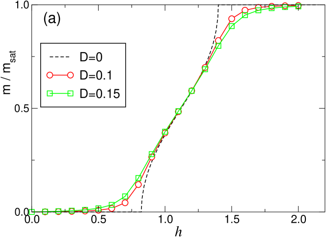
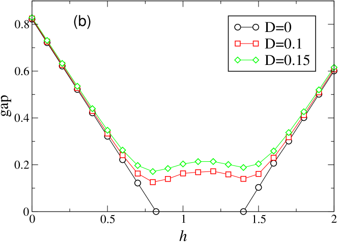
Figure 3: (Color online) Magnetization (a) and gap (b) vs (reduced) magnetic field for finite $D=0.1$ and $D=0.15$, compared to the $D=0$ case, computed on a $2\times 12$ ladder. Note that the $h=h_{c,1}$ singularity at $D=0$ disappears for finite $D$. (The behavior of the gap at $D=0$ is schematic). All energies are in units of $J_{\perp}$.

As mentioned in previous studies miyahara06_dm ; capponi06_ladder_dm , the DM term has been shown to produce a smooth magnetization curve, even for finite clusters, and a gap above $h_{c1}$. For convenience we reproduce here in Fig. 3(a) and (b) the (reduced) magnetization curve and the gap, respectively, as a function of magnetic field for $D=0.1$ and $D=0.15$, values of the DM interaction that we shall consider later on, and also for $D=0$, for comparison.

In the following, for simplicity, we shall focus on the special field such that $m=0.5m_{sat}$. From direct inspection of the magnetization curve, one gets $h\sim 1.1J_{\perp}$ note_h , almost independently of the value of $D$ since all curves seem to cross at his point. Note that, for such a field, bosonization predicts $K=3/4$ and four breathers.

III.2 Low energy spectra: solitons and bound states

Prior to the calculation of the Raman spectrum, it is interesting and useful to first explore the structure of the low energy spectrum. The clusters being periodic (ring geometry), one can take full advantage of the lattice translation symmetry (the unit cell contains two rungs) so that eigenstates are labelled according to their momentum along the legs. We shall focus here on the $q=0$ sector which is relevant in an optical experiment. As a consequence of the $C_{2v}$ symmetry, the $q=0$ states can be split in four separate symmetry sectors $(p,i)=(\pm,\pm)$, corresponding to $\pm 1$ characters, respectively. Although the Raman spectrum will only involve finite excitations belonging to the $(+,+)$ sector (the Raman operator bears the full lattice symmetry), it is useful to consider the four possible symmetry sectors. Before presenting our results about the four spectra, it is necessary to briefly discuss the possible connection of the above quantum numbers $p$ and $i$ defined for the lattice model with symmetries of the bosonized effective model. First, we note that parity corresponds also to a symmetry of the bosonized hamiltonian and of the Sine-Gordon model. In contrast, under the above inversion symmetry, the bosonized Hamiltonian is not invariant by rather transforms according to $D\rightarrow-D$ and $\theta\rightarrow\theta+\pi$ corresponding to a discrete gauge symmetry (the notion of “even” and “odd” sites disappears in the long wavelength limit). Therefore, the excitations of the bosonized Hamiltonian can only be classified according to $p=\pm$. As we discussed in Sec. II.2, the states in the field theory can only be characterized by their parity. We recall that we have found that linear combinations of one soliton and one antisoliton states could be either odd or even under parity, whereas breathers had to be even under parity. These simple symmetry-based considerations will in fact be quite useful for a precise identification of the various eigenstates found in the numerics.

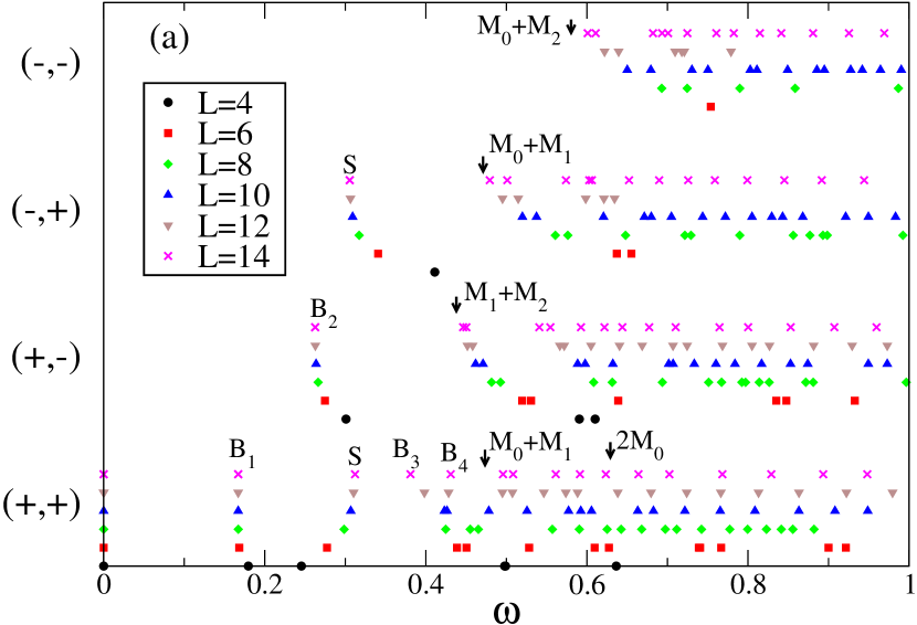
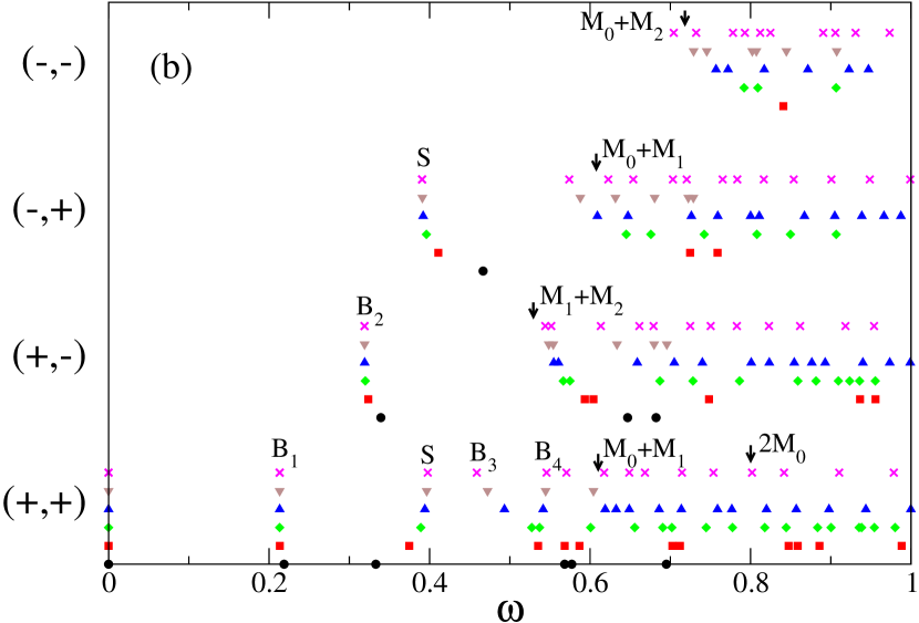
Figure 4: (Color online) Low-energy spectra in the four different $(p,i)$ symmetry sectors for $2\times L$ ladders, $L$ ranging from $L=4$ to $L=14$ according to color/symbol codes shown on the plots, and for $D=0.1$ (a) and $D=0.15$ (b). All energies are measured from the GS energy ($E=0$). Full (LAPACK) diagonalization (small size $L=4,6$), Lanczos and/or Davidson ED ($L=8,10,12,14$) have been performed note_Lanczos . The tentative onsets of the 2-particle continua are indicated by arrows.

We have computed the low-energy spectrum in each symmetry sector of $2\times L$ periodic ladders with $L=4,6,8,10,12$ and $14$. Results for $D=0.1$ and $D=0.15$ are shown on Fig. 4. At low energy, well-defined discrete energy levels clearly saturate to constant values for increasing system sizes. Remarkably, we observe that these states remain separated from the rest of the spectrum which can be characterized as a ”continuum” from the accumulation of levels appearing with increasing cluster size. The discrete levels then correspond either to the soliton or to the breathers of the previous Sections to which we now try to make a precise assignment. To do so, we first notice that two of these levels in the $(+,+)$ and $(-,+)$ sectors are almost degenerate and might correspond to the even and odd parity soliton excitations (see above). As shown in Fig. 5(a), a finite size scaling analysis indeed proves that the ratio of these frequencies converge to 1 in the thermodynamic limit so that these levels can indeed be assigned to the solitons in Fig. 4.

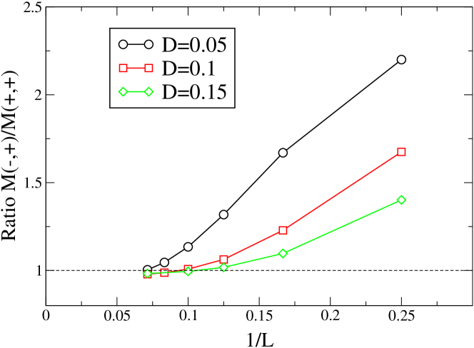
Figure 5: (Color online) Ratio of the two quasi-degenerate excited states in the $(+,+)$ and $(-,+)$ sectors (labelled as “S” in Fig. 4) as a function of inverse system size for different values of $D$ (as indicated on the plot).

After having identified the soliton level (of energy $M_{0}$), we can also safely identify the lowest energy excitation (which is well separated from the rest of the spectrum) as the $B_{1}$ breather of the SG model. We now tentatively assign the remaining discrete levels as $B_{2}$, $B_{3}$ and $B_{4}$, as shown in Fig. 4, and provide a refined analysis that validates this initial guess. First, we note that all suspected breathers indeed correspond to $p=+$ as expected from the SG theory. Secondly, we use the soliton and $B_{1}$ levels as “references” for the identification of the rest of the low-energy spectrum by performing the following analysis: from Eq. (11) of the previous bosonization approach, one expects that the following combinations of the mass ratios,

$$R_{1,2} = \left(\frac{M_{1}}{2M_{0}}\right)^{2}+\left(\frac{M_{2}}{2M_{1}}\right)^{2}\,,$$

$$R_{1,3} = \frac{1}{3}\frac{M_{3}}{M_{1}}+\frac{4}{3}\left(\frac{M_{1}}{2M_{0}}\right)^{2}\,,$$ (38)

converge to $1$ in the limit $D\rightarrow 0$. Such relations can then be considered as useful “consistency checks” of our initial assignments. We have plotted $R_{1,2}$ and $R_{1,3}$ in Fig. 6 as a function of $D$ and for different systems sizes. These plots are indeed consistent with the fact that $R_{1,2}\rightarrow 1$ and $R_{1,3}\rightarrow 1$ for $L\rightarrow\infty$ and (then) $D\rightarrow 0$, validating the assignments of the $B_{2}$ and $B_{3}$ breathers. As far as $B_{4}$ is concerned, its identification is more risky but still very plausible, at least for $D\geq 0.1$. Lastly, we note that, as seen in Fig. 4, simple kinematic rules can be used to combine two of the above excitations (summing up their energies) and lead to the right order of magnitude for the two-particle thresholds (shown by arrows in Fig. 4) as well as the correct quantum numbers..

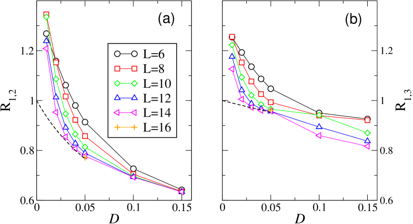
Figure 6: (Color online) $R_{1,2}$ (a) and $R_{1,3}$ (b) of Eq. (38) as a function of $D$ for different systems sizes (as indicated on the plot). The expected $L\rightarrow\infty$ extrapolation is tentatively sketched as a dashed line. The magnetic field is such that $m=0.5\,m_{\rm sat}$ and $D$ is measured in units of $J_{\perp}$.

As a last check, we have considered another (naive) alternative for the $B_{3}$ level as the onset of a 2-particle continuum made of independent $B_{1}$ excitations. However, the extrapolation of the $M_{3}/2M_{1}$ ratio (not shown) in the thermodynamic limit is inconsistent with $M_{3}/2M_{1}$ being exactly 1 for all values of $D$. This gives additional credit to our previous assignments and suggests the absence of a continuum at $2M_{1}$.

III.3 Raman scattering and spectral weight

We now turn to the calculation of the Raman spectrum and investigate the effect of the DM interaction.

It is physically instructive to write the ($T=0$) Raman spectral function in the Lehmann’s representation,

$$I_{R}(\omega) = -\frac{1}{\pi}\Im m\langle 0|\hat{O}_{R}\,\frac{1}{\omega-H+E_{0}+i0^{+}}\,\hat{O}_{R}|0\rangle$$ (39)

$$= \sum_{p}|\langle p|\hat{O}_{R}|0\rangle|^{2}\delta(\omega-(E_{p}-E_{0}))\,,$$ (40)

in terms of the physical excited states $|p\rangle$ of excitation energies $E_{p}-E_{0}$. When the Hamiltonian is isotropic in spin space, since the Raman operator is SU(2) spin-symmetric, it physically describes singlet excitations or, more picturially, “double magnon” excitations. In our case, because of the Hamiltonian anisotropy, the total spin is no longer a good quantum number and the only remaining symmetries (apart from the obvious conservation of the full polarisation $m$) are the space group symmetries discussed above. Operators involving light scattering (like the Raman operator) are translational invariant (on the scale of the lattice spacing) and so involve only $q=0$ excitations. In addition, for light in-coming and out-going polarizations along high-symmetry directions (see later), the Raman operator bears the full lattice symmetry so that the Lehmann sum only contains $(+,+)$ excited states. However, the actual spectral weight might depend strongly on the polarisations. Note that the latter selection rule exclude the $B_{2}$ breather from the Raman spectrum.

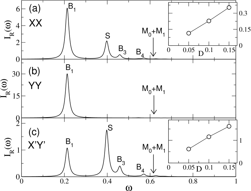
Figure 7: Raman spectra, computed on a $L=14$ cluster, for the three different polarizations XX, YY and X’Y’ (see text) and for $D=0.15$ and a magnetic field such that $m=0.5m_{\rm sat}$. The spurious $\omega=0$ peak has been subtracted (see text). Note that a small imaginary part $\epsilon=0.01$ in the frequency has been used to give a small width to the low-energy delta-peaks. The corresponding weights of these peaks are shown in Fig. 8 as a function of system size. Insets: relative weight of the S state with respect to the B₁ one vs $D$, compatible with a vanishing S intensity as $D\rightarrow 0$

.

We have used a standard Lanczos technique to compute $I_{R}(\omega)$ on finite size clusters up to $L=14$. Within the Lanczos scheme, dynamical correlations can be conveniently expressed as simple continued fractions starting from Eq. (39). The spectral weights can also be exactly computed from the coefficients of the continued fractions. We have checked on small sizes that Lanczos and full diagonalizations do give identical results. We have also checked that, in the absence of magnetic field and DM ($h=0$ and $D=0$), our results are compatible with Ref. natsume_ladder_raman, and can be simply interpreted as a large weight located at twice the spin gap (the Raman operator is a spin singlet and light will create 2 triplet excitations as stated above).

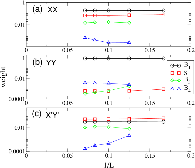
Figure 8: (Color online) Finite-size scaling of the Raman spectral weights of the soliton and the breathers at $D=0.15$ and for a magnetic field such that $m=0.5\,m_{\rm sat}$. All light polarisations XX, YY and X’Y’ are shown. A logarithmic scale is used to reveal the tiny weights in the YY polarisation. For XX and X’Y’ polarisations a sizeable fraction of the overall weight (normalized to 1) is located at higher energies (not shown).

Typical Raman low-energy spectra are shown in Fig. 7 for the same parameters as before. Note that the finite GS expectation values of the Raman operators produce a peak at zero-frequency. To clarify the plots, we have subtracted this trivial contribution (which experimentally is meaningless) and normalized the rest of the spectra so that the total integrated weight is unity. Interestingly, signatures of the soliton and of the $B_{1}$, $B_{3}$ and even $B_{4}$ breathers (all in the $(+,+)$ sector, see Fig. 4) can clearly be seen at low frequency in the XX and X’Y’ spectra. However, for YY polarisation, only the $B_{1}$ peak is sizeable. Note also that the low-energy integrated weight (let us say, up to $\omega\sim J_{\perp}\equiv 1$) depends significantly on the light polarisation. This is directly linked to a large transfer of weight to/from the high-energy region, namely above $\sim 2J_{\perp}$ (not shown), when changing the light polarisation. We have also carried out a finite size scaling analysis of the weights associated to each of the discrete levels, as shown in Fig. 8. We also find that (for the same parameters as before) the relative weight of the S state with respect to e.g. the B1 breather is 0.35, 0.23 and 0.11 for $D=0.15$, $D=0.1$ and $D=0.05$ respectively, e.g. in the XX polarization (see inset of Fig. 7). This shows that the relative weights of the peaks are rather sensitive to the parameter $D$. Our results show small finite size effects and hence strongly suggest that all the sizeable peaks in Fig. 7 survive in the thermodynamic limit.

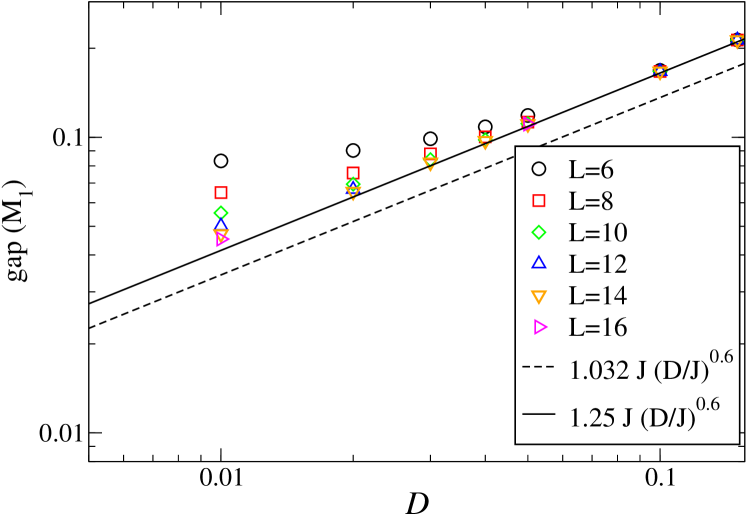
Figure 9: (Color online) Evolution of the gap ($M_{1}$) as a function of $D$ for a magnetic field such that $m=0.5\,m_{\rm sat}$ (log scale). The results for several lengths are reported and the extrapolation for infinite size is consistent with a $D^{3/5}$ behavior (continuous line). The bosonization results shown as a dashed line differs only by a multiplicative factor of order 1.25. All energies are in units of $J_{\perp}$.

Lastly, we come back to the issue of the gap which is plotted in Fig. 3(b). From the previous analysis this gap corresponds in fact to the excitation energy $M_{1}$ of the $B_{1}$ breather. Its behavior as a function of the DM interaction is shown in Fig. 9 and compared to the bosonization prediction $\simeq 1.03J_{\parallel}(D/J_{\parallel})^{3/5}$. Apart from a slightly different multiplicative factor, the agreement between bosonization and (extrapolated) numerical results is excellent.

III.4 Discussion

To conclude this Section, we would like to discuss in more details the comparison of the Raman spectra obtained from exact diagonalization and from bosonization and mapping to the quantum sine-Gordon model.

In the quantum sine-Gordon model, neither operator $\partial_{x}\phi$ nor $\cos\theta$ can change the number of solitons. Thus, they can have non-vanishing matrix elements only between the ground state and the states having an equal number of solitons and antisolitons and any number of breather. As a result, the Raman intensities predicted from the sine-Gordon model in Sec. II.3 are in partial disagreement with the ones obtained from ED if the state S on Fig. 4 is identified with a sine-Gordon soliton. There are three different possibilities to resolve this discrepancy. The first one is that the state S is actually the second breather B₂ of the quantum sine Gordon model. This is compatible with its symmetry since there is one such state in the $(+,+)$ sector. This is also compatible with the observed decrease of the weight of the S peak as $D$ is decreased, as such a behavior is predicted by Eq. (26). In that scenario, the ratio of the masses do not agree with the quantum sine Gordon prediction. The latter result, however, may result from having relatively large gaps that make the continuum limit unjustified. However, in this scenario, we have to understand why there is a state degenerate with the second breather in the sector $(-,+)$.

The second possibility is that the expression (20), which is valid for $J_{\perp}/J_{\parallel}\to\infty$ has corrections of order $(D/J_{\perp})^{m}$ with $m$ an integer coming from higher order virtual processes. If these higher order correction terms contain an operator such as $(-1)^{n}\tau_{n}^{z}$ or $\tau_{n}^{x,y}$ the bosonized form of which are repectively $\cos 2\phi$, $\cos\theta\cos 2\phi$ and $\cos\theta\sin 2\phi$, the Raman operator will contain soliton creation/annihilation operators. This scenario could explain the presence of the peak, while preserving the identification of the state S on Fig. 4 as a soliton. Moreover, this scenario is also compatible with the decrease of the weight in the peak S as $D$ is decreased. Note however that, in this appealing scenario, a question remains: why is the B2 breather odd w.r.t. the inversion symmetry in contrast to the other breathers ? Solving this puzzle unfortunately requires to go beyond the sine-Gordon model (10) which does not exhibit such a symmetry.

The third possibility is that the antisymmetric modes discussed in Sec. II.1 are also contributing to the spectrum of Fig. 4 when $D\sim J_{\parallel}$ even at energy scales small compared to $J_{\perp}$. In that case, the continuum field theory method of Sec. II.2 would be useless to understand the spectra as it implicitely assumes that antisymmetric modes are excited only for energies comparable with $J_{\perp}$. The fuller theory of Sec. II.1 would also be of limited usefulness as the resulting generalized sine-Gordon model discussed in II.1 is non-integrable and thus does not permit to locate breather type excitations.

IV Conclusion

Although the theoretical interpretation of the Raman intensities obtained numerically at intermediate coupling in terms of the solitons and breather of the weak coupling sine-Gordon theory is still a partially open problem, from the point of view of experiment, we can safely conclude that in a two-leg ladder with Dzialoshinskii-Moriya interaction, the presence of a gap in the magnetized phase gives rise to bound states observable in magnetic Raman scattering. In the case of CuHpCl, earlier studies showed that typical parameters like $J_{\parallel}=0.2$ (as used in the numerics) and $D\simeq 0.05$ (all in units of $J_{\perp}$) give a fair description of the magnetization curve miyahara06_dm ; capponi06_ladder_dm and of the specific heat in an applied magnetic field capponi06_ladder_dm . Hence, the above investigation of Raman magnetic scattering (based on analytic and numerical techniques) clearly establishes that, for light polarization along the legs, at least two bound states should be visible, while at least a single bound state should be seen for light polarized along the rungs. We also expect that the spectral weight of the continuum predominantly appears at energies larger than typically $\sim 2J_{\perp}$ i.e., in the case of CuHpCl, above $\sim 3$ meV (although the “theoretical” onset of the continuum is located just above the bound states as predicted by the SG description). In other words, a “pseudo-gap” should form between the bound states and $\sim 2J_{\perp}$. In the particular case of light polarized along the rungs, we further note that the bound state(s) alone should exhaust most of the overall spectral weight. We therefore believe that Raman scattering experiments should provide clear fingerprints of the existence of finite Dzialoshinskii-Moriya interaction in low-dimensional magnets.

- (1) E. Dagotto and T. M. Rice, Science 271, 618 (1996), and references therein.
- (2) E. Dagotto, Rep. Prog. Phys. 62, 1525 (1999).
- (3) T. M. Rice, S. Gopalan, and M. Sigrist, Europhys. Lett. 23, 445 (1993).
- (4) M. Takano et al., Phys. Rev. Lett. 73, 3463 (1994).
- (5) F. D. M. Haldane, Phys. Rev. Lett. 50, 1153 (1983).
- (6) R. Chitra and T. Giamarchi, Phys. Rev. B 55, 5816 (1997).
- (7) A. Furusaki and S.-C. Zhang, Phys. Rev. B 60, 1175 (1999).
- (8) T. Giamarchi and A. M. Tsvelik, Phys. Rev. B 59, 11398 (1999).
- (9) T. Nikuni, M. Oshikawa, A. Oosawa, and H. Tanaka, Phys. Rev. Lett. 84, 5868 (2000).
- (10) M. Clémancey et al., Phys. Rev. Lett. 97, 167204 (2006).
- (11) B. Chiari, O. Piovesana, T. Tarantelli, and P. F. Zanazzi, Inorg. Chem. 29, 1172 (1990).
- (12) G. Chaboussant et al., Phys. Rev. B 55, 3046 (1997).
- (13) G. Chaboussant et al., Phys. Rev. Lett. 80, 2713 (1998).
- (14) G. Chaboussant et al., Eur. Phys. J. B 6, 167 (1998).
- (15) I. Dzyaloshinskii, J. Phys. Chem. Solids 4, 241 (1958).
- (16) T. Moriya, Phys. Rev. 120, 91 (1960).
- (17) M. B. Stone et al., Phys. Rev. B 65, 064423 (2002).
- (18) S. Miyahara et al., Phys. Rev. B 75, 184402 (2007).
- (19) S. Capponi and D. Poilblanc, Phys. Rev. B 75, 092406 (2007).
- (20) P. A. Fleury and R. Loudon, Phys. Rev. 166, 514 (1968).
- (21) T. Moriya, J. Appl. Phys. 39, 42 (1968).
- (22) T. Giamarchi, Quantum Physics in One Dimension (Oxford University Press, Oxford, 2004).
- (23) A. O. Gogolin, A. A. Nersesyan, and A. M. Tsvelik, Bosonization and Strongly Correlated Systems (Cambridge University Press, Cambridge, 1999).
- (24) N. Nagaosa, Quantum Field Theory in Strongly Correlated Electronic Systems, Texts and Monographs in Physics (sprg, Heidelberg, 1999).
- (25) F. Mila, Eur. Phys. J. B 6, 201 (1998).
- (26) M. Oshikawa and I. Affleck, Phys. Rev. Lett. 79, 2883 (1997).
- (27) I. Affleck and M. Oshikawa, Phys. Rev. B 60, 1039 (1999), phys. Rev. B 62, 9200(E) (2000).
- (28) S. P. Strong and A. J. Millis, Phys. Rev. Lett. 69, 2419 (1992).
- (29) S. P. Strong and A. J. Millis, Phys. Rev. B 50, 9911 (1994).
- (30) D. G. Shelton, A. A. Nersesyan, and A. M. Tsvelik, Phys. Rev. B 53, 8521 (1996).
- (31) E. Orignac and T. Giamarchi, Phys. Rev. B 57, 5812 (1998).
- (32) G. I. Japaridze and A. A. Nersesyan, JETP Lett. 27, 334 (1978).
- (33) V. L. Pokrovsky and A. L. Talapov, Phys. Rev. Lett. 42, 65 (1979).
- (34) F. Mila, Eur. Phys. J. B 6, 201 (1998).
- (35) A. Luther, Phys. Rev. B 14, 2153 (1976).
- (36) S. Lukyanov, Phys. Rev. B 59, 11163 (1999).
- (37) S. Lukyanov, Phys. Rev. B 59, 11163 (1999).
- (38) S. Lukyanov and V. Terras, Nucl. Phys. B 654, 323 (2003), hep-th/0206093.
- (39) F. H. L. Essler, Phys. Rev. B 59, 14376 (1999).
- (40) F. H. L. Essler and A. M. Tsvelik, Phys. Rev. B 57, 10592 (1999).
- (41) S. Coleman, Phys. Rev. D 11, 2088 (1975).
- (42) The “soliton” denomination refers to the mathematical property of the Sine-Gordon model although the corresponding physical excitation of the lattice model does not have here any “topological” character.
- (43) R. F. Dashen, B. Hasslacher, and A. Neveu, Phys. Rev. D 11, 3424 (1975).
- (44) See e.g. semi-classical arguments by Roger F. Dashen, Brosl Hasslacher, and André Neveu, Phys. Rev. D 11, 3424 (1975).
- (45) J. Sólyom, Adv. Phys. 28, 209 (1979).
- (46) T. Asano et al., Phys. Rev. Lett. 84, 5880 (2000).
- (47) S. A. Zvyagin, A. K. Kolezhuk, J. Krzystek, and R. Feyerherm, cond-mat/0502393 (unpublished).
- (48) S. Bertaina et al., cond-mat/0501485 (unpublished).
- (49) H. Nojiri, Y. Ajiro, T. Asano, and J.-P. Boucher, New J. Phys. 8, 218 (2006).
- (50) R. Feyerherm et al., J. Phys.: Condens. Matter 12, 8495 (2000).
- (51) A. Wolter et al., Phys. Rev. B 68, 220406(R) (2003).
- (52) M. Kenzelmann et al., Phys. Rev. Lett. 93, 017204 (2004).
- (53) S. A. Zvyagin, A. K. Kolezhuk, J. Krzystek, and R. Feyerherm, Phys. Rev. Lett. 93, 027201 (2004).
- (54) A. U. Wolter et al., Phys. Rev. Lett. 94, 057204 (2005).
- (55) R. Morisaki, T. Ono, H. Tanaka, and H. Uekusa, cond-mat/0607469 (unpublished).
- (56) R. Morisaki, T. Ono, H. Tanaka, and H. Nojiri, cond-mat/0703671 (unpublished).
- (57) A. Luther and I. Peschel, Phys. Rev. B 12, 3908 (1975).
- (58) F. D. M. Haldane, Phys. Rev. Lett. 45, 1358 (1980).
- (59) T. Hikihara and A. Furusaki, cond-mat/0310391 (unpublished).
- (60) M. Abramowitz and I. Stegun, Handbook of mathematical functions (Dover, New York, 1972).
- (61) S. Lukyanov and A. B. Zamolodchikov, Nucl. Phys. B 493, 571 (1997).
- (62) B. S. Shastry and B. I. Shraiman, Phys. Rev. Lett. 65, 1068 (1990).
- (63) P. J. Freitas and R. R. P. Singh, Phys. Rev. B 62, 14113 (2000).
- (64) Y. Natsume, Y. Watabe, and T. Suzuki, J. Phys. Soc. Jpn. 67, 3314 (1998).
- (65) E. Orignac and R. Citro, Phys. Rev. B 62, 8622 (2000).
- (66) P. N. Bibikov, Phys. Rev. B 72, 012416 (2005).
- (67) A. Donkov and A. V. Chubukov, Phys. Rev. B 71, 224431 (2005).
- (68) M. Karowski and P. Wiesz, Nucl. Phys. B 139, 455 (1978).
- (69) G. Mussardo, lectures at the Trieste Summer School on Low-dimensional quantum systems (unpublished).
- (70) D. Controzzi, F. H. L. Essler, and A. M. Tsvelik, in New Theoretical approaches to strongly correlated systems, Vol. 23 of NATO Science Series II. Mathematics, Physics and Chemistry, edited by A. M. Tsvelik (Kluwer Academic Publishers, Dordrecht, 2001), p. 25.
- (71) P. Dorey, hep-th/9810026 (unpublished).
- (72) A. B. Zamolodchikov and A. B. Zamolodchikov, Ann. Phys. (N. Y.) 120, 253 (1979).
- (73) G. Mussardo, Phys. Rep. 218, 215 (1992).
- (74) F. H. L. Essler and A. M. Tsvelik, Phys. Rev. B 57, 10592 (1998).
- (75) F. H. L. Essler, F. Gebhard, and E. Jeckelmann, Phys. Rev. B 64, 125119 (2001).
- (76) H. Babujian, A. Fring, M. Karowski, and A. Zapletal, Nucl. Phys. B 538, 535 (1999), hep-th/9805185.
- (77) H. Babujian and M. Karowski, Nucl. Phys. B 620, 407 (2002), hep-th/0105178.
- (78) S. Lukyanov, Mod. Phys. Lett. A 12, 2543 (1997), hep-th/9703190.
- (79) F. A. Smirnov, Form Factors in Completely Integrable Models of Quantum Field Theory (World Scientific, Singapore, 1992).
- (80) Strictly speaking, this property is only true within the SG description.
- (81) Using values as and , typical of CuHpCl, one gets Tesla.
- (82) Contrary to the Davidson algorithm, in the Lanczos procedure a careful inspection of the evolution of the spectrum with the iteration number is necessary to sort out the “ghosts” states.