Lévy Statistics and Anomalous Transport: Lévy flights and Subdiffusion

Glossary

Ageing.

A dynamical process involving a long-tailed waiting time distribution $\psi(t)\sim\tau^{\alpha}t^{-1-\alpha}$ ($0<\alpha<1$) does not possess a characteristic time scale $\int_{0}^{\infty}t\psi(t)dt$ separating microscopic and macroscopic times. Instead, such a process exhibits distinct memory, such that the now-state of the system is strongly influenced by its state in the past. When the system is prepared at some time $t_{0}<0$ and the measurement starts at $t=0$, this means that the result of the measurement depends on the time $t_{0}$ even until rather long times.

Anomalous diffusion.

Under anomalous diffusion we understand here deviations of the linear time dependence $\langle x^{2}(t)\rangle=2Kt$, of the mean squared displacement in absence of an external bias, in the form of a power-law: $\langle x^{2}(t)\rangle=2K_{\zeta}t^{\zeta}$. Here, $K_{\zeta}$ is the anomalous diffusion constant of dimension $\mathrm{cm}^{2}/\mathrm{sec}^{\zeta}$. In the range $0<\zeta<1$, we deal with subdiffusion, whereas $\zeta>1$ describes superdiffusion. Lévy flights have a diverging mean squared displacement.

Continuous time random walk.

Continuous time random walk theory describes a random motion by assigning each jump a jump length $x$ and a waiting time $t$ elapsing in between two successive jumps, drawn from the two probability densities $\lambda(x)$ and $\psi(t)$, respectively. The two densities $\lambda$ and $\psi$ fully specify the probability density function $P(x,t)$ describing the random process. In Fourier-Laplace space, the propagator follows as $P(k,u)=u^{-1}\psi(u)/[1-\psi(u)\lambda(k)]$.

Fourier and Laplace transforms.

Linear partial differential equations are often conveniently solved using integral transforms of the Laplace and Fourier type. Moreover, the definitions of the fractional operators used in the text correspond to Laplace and Fourier convolutions, such that these transformations also become useful there. The Laplace transform of a function $f(t)$ is defined as

$$f(u)\equiv\mathscr{L}\left\{f(t);u\right\}=\int_{0}^{\infty}f(t)e^{-ut}dt,$$

while the Fourier transform of $g(x)$ reads

$$g(k)\equiv\mathscr{F}\left\{g(x);k\right\}=\int_{-\infty}^{\infty}g(x)e^{ikx}dx.$$

Note that we denote the transform of a function by explicit dependence on the respective variable. For $u=0$ and $k=0$ the Laplace and Fourier transform is but the average of the function $f$ or $g$, respectively. Tauberian theorems ascertain relations between the original function and its transform. For instance, the small $u$ behaviour $f(u)\sim 1-(u\tau)^{\alpha}$ implies the long time scaling $f(t)\sim\tau^{\alpha}/t^{1+\alpha}$. See Refs. Hughes (1995); Feller (1971) for details.

Fractional differintegration.

The multiple derivative of an integer power is $d^{m}x^{n}/dx^{m}=n!/(n-m)!x^{n-m}$ for $m\geq n$. The result is zero if $m>n$. Replacing the factorials by the $\Gamma$-function, one can generalise this relation to ${}_{0}D_{x}^{q}x^{p}=\Gamma(1+p)t^{p-q}/\Gamma(1+p-q)$. In particular, this includes the fractional differentiation of a constant, ${}_{0}D_{x}^{q}1=x^{-q}/\Gamma(1-q)$, that does no longer vanish. Fractional differentiation was first mentioned by Leibniz in a letter to de l’Hospital in 1695. The Riemann-Liouville fractional operator used in the following is a similarly straightforward generalisation of the Cauchy multiple integral, followed by regular differentiation.

Lévy flight.

A Lévy flight is a special type of continuous time random walk. Its waiting time distribution is narrow for instance, Poissonian with $\psi(t)=\tau^{-1}\exp(-t/\tau)$, and the resulting dynamics therefore Markovian. The jump length distribution of a Lévy flight is long-tailed: $\lambda(x)\sim\sigma^{\mu}|x|^{-1-\mu}$, with $0<\mu<2$, such that no second moment exists. The resulting PDF is a Lévy stable law with Fourier transform $P(k,t)=\exp\left(-K^{(\mu)}t|k|^{\mu}\right)$.

Lévy stable laws.

The generalised central limit theorem states that the properly normalised sum of independent, identically distributed random variables with finite variance converges to a Gaussian limit distribution. A generalisation of this theory exists for the case with infinite variance, namely, the generalised central limit theorem. The related distributions are the Lévy stable laws, whose density in the simplest case have the characteristic function $p(k)=\int_{-\infty}^{\infty}p(x)\exp(ikx)dx$ (Fourier transform) of the form $p(k)=\exp\left(-c|k|^{\mu}\right)$, with $0<\mu<2$. In direct space, this corresponds to a power-law asymptotic $p(x)\simeq c|x|^{-1-\mu}$. In the limit $\mu=2$, the universal Gaussian distribution is recovered.

Lévy walks.

In contrast to Lévy flights, Lévy walks possess a finite mean squared displacement, albeit having a broad jump length distribution. This is possible by the introduction of a time penalty for long jumps through a coupling $\lambda(x)p(t|x)$ between waiting times and jump lengths, such that long jumps involve a longer waiting time. For instance, a $\delta$-coupling of the form $\frac{1}{2}\lambda(x)\delta(|x|-vt)$ is often chosen, such that $v$ plays the role of a velocity.

Strange kinetics.

Often, deviations from exponential relaxation patterns $\exp(-t/\tau)$ and regular Brownian diffusion are observed. Instead, non-exponential relaxation, for instance, of the stretched exponential form $\exp\left(-[t/\tau]^{\alpha}\right)$ ($0<\alpha<1$) or of the inverse power-law form $t^{-\zeta}$, are observed, or anomalous diffusion behaviour is found.

Weak ergodicity breaking.

In a system with a broadly distributed waiting time with diverging characteristic time scale, a particle can get stuck at a certain position for a long time. For instance, for a waiting time distribution of the form $\psi(t)\sim\tau^{\alpha}t^{-1-\alpha}$, the probability of not moving until time $t$ scales as $\tau^{\alpha}t^{-\alpha}$, i.e., decays very slowly. The probability for not moving is therefore appreciable even for long times. A particle governed by such a $\psi(t)$ even at stationarity does not equally explore a different domains of phase space.

I Definition and importance of anomalous diffusion

Classical Brownian motion characterised by a mean squared displacement

$$\langle x^{2}(t)\rangle=2Kt,$$ (1)

growing linear in time in absence of an external bias is the paradigm for random motion. Note that we restrict our discussion to one dimension. It quantifies the jittery motion of coal dust particles observed by Dutchman Jan Ingenhousz in 1785 ingenhousz , the zigzagging of pollen grain in solution reported by Robert Brown in 1827 brown , and possibly the dance of dust particles in the beam of sunlight in a stairwell so beautifully embalmed in the famed poem by Lucretius carus . In general, Brownian motion occurs in simple, sufficiently homogeneous systems such as simple liquids or gasses. In the continuum limit, Brownian motion is governed by the diffusion equation

$$\frac{\partial P(x,t)}{\partial t}=K\frac{\partial^{2}}{\partial x^{2}}P(x,t)$$ (2)

for the probability density function (PDF) $P(x,t)$ describing the probability $P(x,t)dx$ to find the particle at a position in the interval $x,\ldots,x+dx$ at time $t$. For a point-like initial condition $P(x,0)=\delta(x)$, the solution becomes the celebrated Gaussian PDF

$$P(x,t)=\frac{1}{\sqrt{4\pi Kt}}\exp\left(-\frac{x^{2}}{4Kt}\right).$$ (3)

The diffusion constant $K$ fulfils the Einstein-Stokes relation $K=k_{B}T/(m\eta)$, where $k_{B}T$ is the Boltzmann energy at temperature $T$, $m$ is the mass of the test particle, and $\eta$ the friction coefficient. This relation between microscopic and macroscopic quantities was used for the determination of the Avogadro number by Perrin perrin . Examples of Perrin’s recorded random walks and the jump length distribution constructed from the data for a time increment of 30 sec are shown in Fig. 1. Fig. 2 displays time traces of the Brownian motion of a small mirror in air that lead to an amazingly accurate determination of the Avogadro number by Keppler, for two different ambient pressures kappler .

Figure 1: Random walk trajectories of putty particles in water recorded by Perrin perrin1 . Left: three designs obtained by tracing a small grain of putty at intervals of 30sec. Right: the starting point of each motion event is shifted to the origin. The figure illustrates the continuum approach of the jump length distribution if only a large number of jumps is considered.

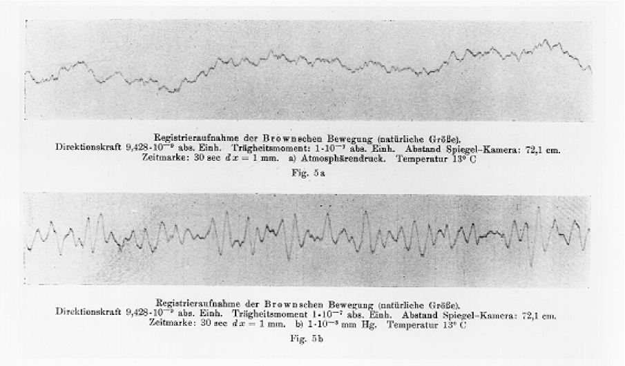
Figure 2: Erroneous behaviour of Brownian motion made visible in a high–precision measurement. Data from an Edelmann recorder, obtained by Kappler in 1931 kappler . Kappler monitored the Brownian motion of a small mirror (surface approx. $1{\rm mm}^{2}$), suspended from a fine quartz thread (several cm long and some $\mu$m thick). The mean squared of the torsional displacement, $\overline{\varphi^{2}}$, follows the relation $D\overline{\varphi^{2}}=k_{B}T$, where $D$ is the directional force of the suspension kappler . The facsimiles show three different realisations. From his data, Kappler obtained the Avogadro–Loschmidt number $N_{L}=60.59\cdot 10^{22}\pm 1\%$, to a remarkable accuracy.

However, in many systems deviations from the linear behaviour (1) are observed bouchaudgeorges ; Metzler and Klafter (2000, 2004); soklablu ; zaslavsky ; chechkinreview ; physicstoday . These deviations can assume the power-law form

$$\langle x^{2}(t)\rangle=2K_{\zeta}t^{\zeta}.$$ (4)

For $0<\zeta<1$, we observe subdiffusion. Prominent examples of subdiffusion include charge carrier transport in amorphous semiconductors pfister ; Montroll and Scher (1973), diffusion of chemicals in subsurface aquifers grl , the motion of beads in actin gels weitz , motion in chaotic maps Zumofen and Klafter (1993); eli , or the subdiffusion of biomacromolecules in cells golding ; just to name a few [compare Metzler and Klafter (2004) for more details]. Subdiffusion of this type is characterised by a long-tailed waiting time PDF $\psi(t)\simeq t^{-1-\alpha}$, corresponding to the time-fractional diffusion equation

$$\frac{\partial P(x,t)}{\partial t}=K_{\alpha}\,{}_{0}D_{t}^{1-\alpha}\frac{\partial^{2}}{\partial x^{2}}P(x,t),$$ (5)

with the fractional Riemann-Liouville operator Samko et al. (1993); oldham ; Podlubny (1998)

$${}_{0}D_{t}^{1-\alpha}P(x,t)=\frac{1}{\Gamma(\alpha)}\frac{\partial}{\partial t}\int_{0}^{t}\frac{P(x,t^{\prime})}{(t-t^{\prime})^{1-\alpha}}dt^{\prime}$$ (6)

From the latter definition, it becomes apparent that subdiffusion corresponds to a slowly decaying memory integral in the dynamical equation for $P(x,t)$.

The lack of a characteristic time scale (i.e., the divergence of $\int_{0}^{\infty}t\psi(t)dt$) of the waiting time PDF $\psi(t)\simeq t^{-1-\alpha}$ no longer permits to distinguish microscopic and macroscopic events. This causes that the diffusing particle can get stuck at a certain position for very long times, quantified by the sticking probability $\phi(t)=\int_{t}^{\infty}\psi(t^{\prime})dt^{\prime}$ of not moving. The PDF $P(x,t)$ exhibits characteristic cusps at the location where the particle was initially released and, in the presence of an external drift, growing asymmetry. Moreover, a process whose measurement begins at $t=0$ depends on the preparation time at some prior time, the so-called ageing eli ; bouchaudage . Another effect in this context is that a particle no longer evenly distributes in a certain space, such that despite the existence of stationary states a weak ergodicity breaking occurs eliweb ; bouchaudweb ; michaelweb .

Contrasting a subdiffusing particle are Lévy flights (LFs), that are based on a waiting time PDF with finite characteristic time but a jump length distribution $\lambda(x)\simeq|x|^{-1-\mu}$ ($0<\mu<2$) with diverging variance $\int_{-\infty}^{\infty}|x|^{2}\lambda(x)dx$. The diffusion equation for an LF becomes generalised to the space-fractional diffusion equation

$$\frac{\partial P(x,t)}{\partial t}=K^{(\mu)}\frac{\partial^{\mu}}{\partial|x|^{\mu}}P(x,t),$$ (7)

where the fractional Riesz-Weyl operator is defined through its Fourier transform $\mathscr{F}\left\{\partial^{\mu}/\partial|x|^{\mu}P(x,t)\right\}=-|k|^{\mu}P(k,t)$. In Fourier space, one therefore recovers immediately the characteristic function $P(k,t)=\exp\left(-K^{(\mu)}|k|^{\mu}t\right)$ of a symmetric Lévy stable law. As can be seen from Eq. (7) LFs are Markovian processes. However, their trajectory now has a fractal dimension $d_{f}=\mu$ and is characterised by local search changing with long excursions, see Fig. 3. This property has been shown to be a better search strategy than Brownian motion, as it oversamples less Lomholt et al. (2005); stanleysearch . In fact, animals like albatross albatross , spider monkeys spider , jackals jackals , and even plankton plankton and bacteria bacteria were claimed to follow Lévy search strategies. LFs also occur in diffusion in energy space sms , or in optical lattices opticallattice . Due to the clustering nature of their trajectory, LFs also exhibit a form of ergodicity breaking lutzweb .

Figure 3: Trajectories of Brownian motion (left) and a Lévy flight of index $\mu=1.5$ (right), both with the same number ($\simeq 7000$) of steps. The long sojourns and clustering appearance of the Lévy flight are distinct.

II Introduction

For sums of independent, identically distributed random variables with proper normalisation to the sample size, the generalised central limit theorem guarantees the convergence of the associated probability density to a Lévy stable density even though the variance of these random variables diverges Lévy (1954); Feller (1971); Gnedenko and Kolmogorov (1954); Hughes (1995); uchaikin . Well-known examples for Lévy stable densities are the one-sided (defined for $x\geq 0$) Lévy-Smirnov distribution

$$f_{1/2,-1/2}(x)=\sqrt{\frac{1}{2\pi x^{3}}}\exp\left(-\frac{1}{2x}\right),$$ (8)

related to the first passage time density of a Gaussian random walk process of passing the origin (see below), and the Cauchy (or Lorentz) distribution

$$f_{1,0}(x)=\frac{1}{\pi\left(1+x^{2}\right)}.$$ (9)

In general, an Lévy stable density is defined through its characteristic function of the PDF $f(x)$

$$\varphi(z)\equiv\mathscr{F}\left\{f(x)\right\}=\int_{-\infty}^{\infty}f_{\mu,\beta}(x)e^{ikx}dx$$ (10)

where

$$\log\varphi(z)=-|z|^{\mu}\exp\left\{i\frac{\pi\beta}{2}\mathrm{sign}(z)\right\},$$ (11)

for $\mu\neq 1$. Here, the skewness (or asymmetry) parameter $\beta$ is restricted to the following region:

$$|\beta|\leq\left\{\begin{array}[]{ll}\mu,&\mbox{if }0<\mu<1\\ 2-\mu,&\mbox{if }1<\mu<2.\end{array}\right.$$ (12)

For $\beta=0$, the corresponding Lévy stable density is symmetric around $x=0$, while for $\beta=-\mu$ and $0<\mu<1$, it is one-sided. In general, an Lévy stable density follows the power-law asymptotic behaviour

$$f_{\mu,\beta}(x)\sim\frac{A_{\mu,\beta}}{|x|^{1+\mu}},\,\,\,\mu<2,$$ (13)

with $A_{\mu,\beta}$ being a constant, such that for all Lévy stable densities with $\mu<2$ the variance diverges

$$\langle x^{2}\rangle=\infty.$$ (14)

Conversely, all fractional moments $\langle|x|^{\delta}\rangle<\infty$ for all $0<\delta<\mu\leq 2$. From above definitions it is obvious that the Lévy stable density $f_{2,0}$ corresponds to the Gaussian normal distribution

$$f_{2,0}(x)=\sqrt{\frac{1}{4\pi}}\exp\left(-\frac{1}{4}x^{2}\right)$$ (15)

possessing finite moments of any order. In this limit, the generalised central limit theorem coincides with the more traditional, and universal, central limit theorem.

Brownian motion has traditionally been employed as the dominant model of choice for random noise in continuous-time systems, due to its remarkable statistical properties and its amenability to mathematical analysis. However, Brownian motion is just a single example of the Lévy family. Moreover, it is a very special and somewhat misrepresenting member of this family. Amongst the Lévy family, the Brownian member is the only motion with continuous sample-paths. All other motions have discontinuous trajectories, exhibiting jumps. Moreover, the Lévy family is characterized by selfsimilar motions. Brownian motion is the only selfsimilar Lévy motion possessing finite variance, while all other selfsimilar Lévy motions have an infinite variance.

Random processes whose spatial coordinate $x$ or clock time $t$ are distributed according to an Lévy stable density exhibit anomalies, that is, no longer follow the laws of Brownian motion. Consider a continuous time random walk process defined in terms of the jump length and waiting time distributions $\lambda(x)$ and $\psi(t)$ Montroll and Weiss (1969); Montroll and Scher (1973). Each jump event of this random walk, that is, is characterised by a jump length $x$ drawn from the distribution $\lambda$, and the time $t$ between two jump events is distributed according to $\psi$. (Note that an individual jump is supposed to occur spontaneously.) In absence of an external bias, continuous time random walk theory connects $\lambda(x)$ and $\psi(t)$ with the probability distribution $P(x,t)dx$ to find the random walker at a position in the interval $(x,x+dx)$ at time $t$. In Fourier-Laplace space, $P(k,u)\equiv\mathscr{F}\left\{\mathscr{L}\left\{P(x,t);t\to u\right\};x\to k\right\}$, this relation reads Klafter et al. (1987)

$$P(k,u)=\frac{1-\psi(u)}{u}\frac{1}{1-\lambda(k)\psi(u)},$$ (16)

where $\mathscr{L}\{f(t)\}\equiv\int_{0}^{\infty}\exp(-ut)f(t)dt$. We here neglect potential complications due to ageing effects. The following cases can be distinguished:

(i) $\lambda(x)$ is Gaussian with variance $\sigma^{2}$ and $\psi(t)=\delta(t-\tau)$. Then, to leading order in $k^{2}$ and $u$, respectively, one obtains $\lambda(k)\simeq 1-\sigma^{2}k^{2}$ and $\psi(u)\simeq 1-u\tau$. From relation (16) one recovers the Gaussian probability density $P(x,t)=\sqrt{1/(4\pi Kt)}\exp\{-x^{2}/(4Kt)\}$ with diffusion constant $K=\sigma^{2}/\tau$. The corresponding mean squared displacement grows linearly with time, see Eq. (1). This case corresponds to the continuum limit of regular Brownian motion. Note that here and in the following, we restrict the discussion to one dimension.

(ii) Assume $\lambda(x)$ still to be Gaussian, while for the waiting time distribution $\psi(t)$ we choose a one-sided Lévy stable density with stable index $0<\alpha<1$. Consequently, $\psi(u)\simeq 1-(u\tau)^{\alpha}$, and the characteristic waiting time $\int_{0}^{\infty}t\psi(t)dt$ diverges. Due to this lack of a time scale separating microscopic (single jump events) and macroscopic (on the level of $P(x,t)$) scales, $P(x,t)$ is no more Gaussian, but given by a more complex $H$-function schneider ; Metzler and Klafter (2000, 2004). In Fourier space, however, one finds the quite simple analytical form Metzler and Klafter (2000)

$$P(k,t)=E_{\alpha}\left(-K_{\alpha}k^{2}t^{\alpha}\right)=\sum_{0}^{\infty}\frac{\left(K_{\alpha}k^{2}t^{\alpha}\right)^{n}}{\Gamma(1+\alpha n)}$$ (17)

in terms of the Mittag-Leffler function. This generalised relaxation function of the Fourier modes turns from an initial stretched exponential (KWW) behaviour

$$P(k,t)\sim 1-K_{\alpha}k^{2}t^{\alpha}/\Gamma(1+\alpha)\sim\exp\left\{-K_{\alpha}k^{2}t^{\alpha}/\Gamma(1+\alpha)\right\}$$ (18)

to a terminal power-law behaviour Metzler and Klafter (2000)

$$P(k,t)\sim\Big{(}K_{\alpha}k^{2}t^{\alpha}\Gamma(1-\alpha)\Big{)}^{-1}.$$ (19)

In the limit $\alpha\to 1$, it reduces to the traditional exponential $P(k,t)=\exp(-Kk^{2}t)$ with finite characteristic waiting time. Also the mean squared displacement changes from its linear to the power-law time dependence

$$\langle x^{2}(t)\rangle=2K_{\alpha}t^{\alpha},$$ (20)

with $K_{\alpha}=\sigma^{2}/\tau_{0}^{\alpha}$. This is the case of subdiffusion. We note that in $x,t$ space the dynamical equation is the fractional diffusion equation schneider . In the presence of an external potential, it generalises to the time-fractional Fokker-Planck equation Metzler et al. (1999); Metzler and Klafter (2000, 2004), see also below.

(iii) Finally, take $\psi(t)=\delta(t-\tau)$ sharply peaked, but $\lambda(x)$ of Lévy stable form with index $0<\mu<2$. The resulting process is Markovian, but with diverging variance. It can be shown that the fractional moments scale like Metzler and Nonnenmacher (2002)

$$\langle|x(t)|^{\delta}\rangle\propto\left(K^{(\mu)}t\right)^{\delta/\mu},$$ (21)

were $K^{(\mu)}=\sigma^{\mu}/\tau$. The upper index $\mu$ is chosen to distinguish ^μ from the subdiffusion constant $K_{\mu}$. Note that the dimension of $K^{(\mu)}$ is $\mathrm{cm}^{\mu}/\mathrm{sec}$. From Eq. (16) one can immediately obtain the Fourier image of the associated probability density function,

$$P(k,t)=\exp\Big{\{}-K^{(\mu)}|k|^{\mu}t\Big{\}}.$$ (22)

From Eq. (11) this is but a symmetric Lévy stable density with stable index $\mu$, and this type of random walk process is most aptly coined a Lévy flight. A Lévy flight manifestly has regular exponential mode relaxation and is in fact Markovian. However, the modes in position space are no more sharply localised like in the Gaussian or subdiffusive case. Instead, individual modes bear the hallmark of an Lévy stable density, that is, the diverging variance. We will see below how the presence of steeper than harmonic external potentials causes a finite variance of the Lévy flight, although a power-law form of the probability density remains.

In the remainder of this paper, we deal with the physical and mathematical properties of Lévy flights and subdiffusion. While mostly we will be concerned with the overdamped case, in the last section we will address the dynamics in velocity space in the presence of Lévy noise, in particular, the question of the diverging variance of Lévy flights.

III Lévy flights

III.1 Underlying random walk process

To derive the dynamic equation of a Lévy flight in the presence of an external force field $F(x)=-dV(x)/dx$, we pursue two different routes. One starts with a generalised version of the continuous time random walk, compare Ref. Metzler et al. (1999a) for details; a slightly different derivation is presented in Ref. bamekla .

To include the local asymmetry of the jump length distribution due to the force field $F(x)$, we introduce Metzler et al. (1999a); Metzler (2001) the generalised transfer kernel $\Lambda(x,x^{\prime})=\lambda(x-x^{\prime})\left[A(x^{\prime})\Theta(x-x^{\prime})+B(x^{\prime})\Theta(x^{\prime}-x)\right]$ (and therefore $\Lambda(x,x^{\prime})=\Lambda(x^{\prime};x-x^{\prime})$). As in standard random walk theory (compare Weiss (1994)), the coefficients $A(x)$ and $B(x)$ define the local asymmetry for jumping left and right, depending on the value of $F(x)$. Here, $\Theta(x)$ is the Heaviside jump function. With the normalisation $\int\Lambda(x^{\prime},\Delta)d\Delta=1$, the fractional Fokker-Planck equation (FFPE) ensues Metzler et al. (1999a):

$$\frac{\partial}{\partial t}P(x,t)=\left(-\frac{\partial}{\partial x}\frac{F(x)}{m\eta}+K^{(\mu)}\frac{\partial^{\mu}}{\partial|x|^{\mu}}\right)P(x,t).$$ (23)

Remarkably, the presence of the Lévy stable $\lambda(x)$ only affects the diffusion term, while the drift term remains unchanged Fogedby (1998); fogedby1 ; Metzler et al. (1999a). The fractional spatial derivative represents an integrodifferential operator defined through

$$\frac{\partial^{\mu}}{\partial|x|^{\mu}}P(x,t)=\frac{-1}{2\cos(\pi\mu/2)\Gamma(2-\mu)}\frac{\partial^{2}}{\partial x^{2}}\int_{-\infty}^{\infty}\frac{P(x^{\prime},t)}{|x-x^{\prime}|^{\mu-1}},$$ (24)

for $1<\mu<2$, and a similar form for $0<\mu<1$ Chechkin et al. (2004); Samko et al. (1993); Podlubny (1998). In Fourier space, for all $0<\mu\leq 2$ the simple relation

$$\mathscr{F}\left\{\frac{\partial^{\mu}}{\partial|x|^{\mu}}P(x,t)\right\}=-|k|^{\mu}P(k,t)$$ (25)

holds. In the Gaussian limit $\mu=2$, all relations above reduce to the familiar second-order derivatives in $x$ and thus the corresponding $P(x,t)$ is governed by the standard Fokker-Planck equation.

The FFPE (23) can also be derived from the Langevin equation Fogedby (1998); fogedby1 ; Jespersen et al. (1999); Chechkin et al. (2004)

$$\frac{dx(t)}{dt}=-\frac{1}{m\gamma}\frac{dV(x)}{dx}+\xi_{\mu}(t),$$ (26)

driven by white Lévy stable noise $\xi_{\mu}(t)$, defined through $L(\Delta t)=\int_{t}^{t+\Delta t}\xi_{\mu}\left(t^{\prime}\right)dt^{\prime}$ being a symmetric Lévy stable density of index $\mu$ with characteristic function $p(k,\Delta t)=\exp\left(-K_{\mu}|k|^{\mu}\Delta t\right)$ for $0<\mu\leq 2$. As with standard Langevin equations, $K^{(\mu)}$ denotes the noise strength, $m$ is the mass of the diffusing (test) particle, and $\gamma$ is the friction constant characterising the dissipative interaction with the bath of surrounding particles.

A subtle point about the FFPE (23) is that it does not uniquely define the underlying trajectory Sokolov and Metzler (2004); however, starting from our definition of the process in terms of the stable jump length distribution $\lambda(x)\sim|x|^{-1-\mu}$, or its generalised pendant $\Lambda(x,x^{\prime})$, the FFPE (23) truly represents a Lévy flight in the presence of the force $F(x)$. This poses certain difficulties when non-trivial boundary conditions are involved, as shown below.

III.2 Propagator and symmetries

Figure 4: Cauchy distribution ($\mu=1$) for two times in comparison to the Gaussian ($\mu=2$). We chose $K^{(1)}=K=1$. Note that the Cauchy distribution is narrower at the origin, and after crossing the Gaussian falls off in the much slower power-law fashion.

In absence of an external force, $F(x)=0$, the exact solution of the FFPE is readily obtained as the Lévy stable density $P(k,t)=\exp\left(-K^{(\mu)}|k|^{\mu}t\right)$ in Fourier space. Back-transformed to position space, an analytical solution is given in terms of the Fox $H$-function Metzler and Klafter (2000); wegrimeno ; Jespersen et al. (1999)

$$P(x,t)=\frac{1}{\mu|x|}H^{1,1}_{2,2}\left[\frac{|x|}{\left(K^{(\mu)}t\right)^{1/\mu}}\left|\begin{array}[]{l}(1,1/\mu),(1,1/2)\\ (1,1),(1,1/2)\end{array}\right.\right],$$ (27)

from which the series expansion

$$P(x,t)=\frac{1}{\mu(K^{(\mu)}t)^{1/\mu}}\sum_{\nu=0}^{\infty}\frac{\Gamma([1+\nu]/\mu)}{\Gamma([1+\nu]/2)\Gamma(1-[1+\nu]/2)}\frac{(-1)^{\nu}}{\nu!}\left(\frac{|x|}{(K^{(\mu)}t)^{1/\mu}}\right)^{\nu}$$ (28)

derives. For $\mu=1$, the propagator reduces to the Cauchy Lévy stable density

$$P(x,t)=\frac{1}{\pi\left(K^{(1)}t+x^{2}/[K^{(1)}t]\right)}.$$ (29)

We plot the time evolution of $P(x,t)$ for the Cauchy case $\mu=1$ in Fig. 4 in comparison to the limiting Gaussian case $\mu=2$.

Due to the point symmetry of the FFPE (23) for $F(x)=0$, the propagator $P(x,t)$ is invariant under change of sign, and it is monomodal, i.e., it has its global maximum at $x=0$, the point where the initial distribution $P(x,0)=\delta(x)$ was launched at $t=0$. The latter property is lost in the case of strongly confined Lévy flights discussed below. Due to their Markovian character, Lévy flights also possess a Galilei invariance Metzler and Compte (2000a); Metzler and Klafter (2000). Thus, under the influence of a constant force field $F(x)=F_{0}$, the solution of the FFPE can be expressed in terms of the force-free solution by introducing the wave variable $x-F_{0}t$, to obtain

$$P_{F_{0}}(x,t)=P_{0}\left(x-\frac{F_{0}t}{m\gamma},t\right).$$ (30)

This result follows from the FFPE (23), that in Fourier domain becomes Jespersen et al. (1999)

$$\frac{\partial}{\partial t}P(k,t)=\left(-ik\frac{F_{0}}{m\gamma}-K^{(\mu)}|k|^{\mu}\right)P(k,t),$$ (31)

with solution

$$P(k,t)=\exp\left(-\left[ik\frac{F_{0}}{m\gamma}+K^{(\mu)}|k|^{\mu}\right]t\right).$$ (32)

By the translation theorem of the Fourier transform, Eq. (30) yields. We show an example of the drift superimposed to the dispersional spreading of the propagator in Fig. 5.

Figure 5: Cauchy distribution with $K^{(1)}=1$ advected along a field $F_{0}/(m\gamma)=2$, for different times.

III.3 Presence of external potentials

III.3.1 Harmonic potential

In an harmonic potential $V(x)=\frac{1}{2}\lambda x^{2}$, an exact form for the characteristic function can be found. Thus, from the corresponding FFPE in Fourier space,

$$\frac{\partial}{\partial t}P(k,t)=-\frac{\lambda}{m\gamma}k\frac{\partial}{\partial k}P(k,t)-K^{(\mu)}|k|^{\mu}P(k,t),$$ (33)

by the method of characteristics one obtains

$$P(k,t)=\exp\left(-\frac{m\gamma K^{(\mu)}|k|^{\mu}}{\lambda\mu}\left[1-e^{-\mu\lambda t/(m\gamma)}\right]\right)$$ (34)

for an initially central $\delta$-peak, $P(x,0)=\delta(x)$ Jespersen et al. (1999). This is but the characteristic function of an Lévy stable density with time-varying width. For short times, $1-\exp(-\mu\lambda t/[m\gamma])\sim\mu\lambda t/[m\gamma]$ grows linearly in time, such that $P(k,t)\sim\exp\left(-K^{(\mu)}|k|^{\mu}t\right)$ as for a free Lévy flight. At long times, the stationary solution defined through

$$P_{\mathrm{st}}(k)=\exp\left(-\frac{m\gamma K^{(\mu)}|k|^{\mu}}{\lambda\mu}\right),$$ (35)

is reached. Interestingly, it has the same stable index $\mu$ as the driving Lévy noise. By separation of variables, a summation formula for $P(x,t)$ can be obtained similarly to the solution of the Ornstein-Uhlenbeck process in the presence of white Gaussian noise, however, with the Hermite polynomials replaced by $H$-functions Jespersen et al. (1999).

We note that in the Gaussian limit $\mu=2$, the stationary solution by necessity has to match the Boltzmann distribution corresponding to $\exp\left(-k_{B}Tk^{2}/[2\lambda]\right)$. This requires that the Einstein-Stokes relation $K=k_{B}T/(m\gamma)$ is fulfilled van Kampen (1981). One might therefore speculate whether for a system driven by external Lévy noise a generalised Einstein-Stokes relation should hold, as was established for the subdiffusive case Metzler et al. (1999); Metzler and Klafter (2000). As will be shown now, in steeper than harmonic external potentials, the stationary form of $P(x,t)$ even leaves the basin of attraction of Lévy stable densities.

III.3.2 Steeper than harmonic potentials

To investigate the behaviour of Lévy flights in potentials, that are steeper than the harmonic case considered above, we introduce the non-linear oscillator potential

$$V(x)=\frac{a}{2}x^{2}+\frac{b}{4}x^{4},$$ (36)

that can be viewed as a next order approximation to a general confining, symmetric potential. It turns out that the resulting process differs from above findings if a suitable choice of the ratio $a/b$ is made. For simplicity, we introduce dimensionless variables through

$$x\to x/x_{0};\,\,t\to t/t_{0};\,\,a\to at_{0}/(m\gamma),$$ (37)

where

$$x_{0}=\left(\frac{m\gamma K^{(\mu)}}{b}\right)^{1/(2+\mu)};\,\,t_{0}=\frac{x_{0}^{\mu}}{K^{(\mu)}},$$ (38)

arriving at the FFPE

$$\frac{\partial}{\partial t}P(k,t)+|k|^{\mu}=\left(k\frac{\partial^{3}}{\partial k^{3}}-ak\frac{\partial}{\partial k}\right)P(k,t).$$ (39)

Figure 6: Bimodal stationary probability density $P_{\mathrm{st}}(x)$ from Eq. (40). The maxima are at $\pm\sqrt{1/2}$.

Consider first the simplest case of a quartic oscillator with $a=0$ in the presence of Cauchy noise ($\mu=1$). In this limit, the stationary solution can be obtained exactly, yielding the expression

$$P_{\mathrm{st}}(x)=\frac{1}{\pi}\frac{1}{1-x^{2}+x^{4}}$$ (40)

plotted in Fig. 6. Two distinct new features in comparison to the free Lévy flight, and the Lévy flight in an harmonic potential: (1) Instead of the maximum at $x=0$, one observes two maxima positioned at

$$x_{m}=\pm\sqrt{1/2};$$ (41)

at $x=0$, we find a local minimum. (2) There occurs a power-law asymptote

$$P_{\mathrm{st}}(x)\sim\frac{1}{\pi x^{4}}$$ (42)

for $x\gg 1$; consequently, this stationary solution no longer represents an Lévy stable density, and the associated mean squared displacement is finite, $\langle x^{2}\rangle<\infty$.

A more detailed analysis of Eq. (39) reveals Chechkin et al. (2003, 2004), that (i) the bimodality of $P(x,t)$ occurs only if the amplitude of the harmonic term, $a$, is below a critical value $a_{c}$; (ii) for general $\mu$, the asymptotic behaviour is $P_{\mathrm{st}}(x)\sim\pi^{-1}\sin(\pi\mu/2)\Gamma(\mu)|x|^{-\mu-3}$; (iii) and there exists a finite bifurcation time $t_{c}$ at which the initially monomodal form of $P(x,t)$ acquires a zero curvature at $x=0$, before settling in the terminal bimodal form.

Interestingly, in the more general power-law behaviour

$$V(x)=\frac{|x|^{c}}{c},$$ (43)

the turnover from monomodal to bimodal form of $P(x,t)$ occurs exactly when $c>2$. The harmonic potential is therefore a limiting case when the solution of the FFPE still belongs to the class of Lévy stable densities and follows the generalised central limit theorem. This is broken in a superharmonic (steeper than harmonic) potential. The corresponding bifurcation time $t_{c}$ is finite for all $c>2$ Chechkin et al. (2004). An additional effect appears when $c>4$: there exists a transient trimodal state when the relaxing $\delta(x)$-peak overlaps with the forming humps at $x=\pm x_{m}$. At the same time, the variance is finite, if only $c>4-\mu$, following from the asymptotic stationary solution

$$P_{\mathrm{st}}(x)\sim\frac{\sin(\pi\mu/2)\Gamma(\mu)}{\pi|x|^{\mu+c-1}}.$$ (44)

Details of the asymptotic behaviour and the bifurcations can be found in Refs. Chechkin et al. (2003, 2004). From a reverse engineering point of view, Lévy flights in confining potentials are studied in Eliazar and Klafter (2003).

III.4 First passage and first arrival of Lévy flights

One might naively expect that a jump process of Lévy type, whose variance diverges (unless confined in a steep potential) may lead to ambiguities when boundary conditions are introduced, such as an absorbing boundary at finite $x$. Indeed, it is conceivable that for a jump process with extremely long jumps, it becomes ambiguous how to properly define the boundary condition: should the test particle be absorbed when it arrives exactly at the boundary, or when it crosses it anyplace during a non-local jump?

This question is trivial in the case of a narrow jump length distribution: all steps are small, and the particle cannot jump across a point (in the continuum limit considered herein). For such processes, one enforces a Cauchy boundary condition $P(0,t)=0$ at the point $x=0$ of the absorbing boundary, removing the particle once it hits the barrier after starting at $x_{0}$, where the dynamics is governed by Eq. (23) with $F(x)=0$. Its solution can easily be obtained by standard methods, for instance, the method of images. This is completely equivalent to considering the first arrival to the point $x=0$, expressed in terms of the diffusion equation with sink term:

$$\frac{\partial}{\partial t}\mathscr{P}(x,t)=K\frac{\partial^{2}}{\partial x^{2}}\mathscr{P}(x,t)-p_{\mathrm{fa}}(t)\delta(x),$$ (45)

defined such that $P(0,t)=0$. Note that the quantity $\mathscr{P}$ is no longer a probability density, as probability decays to zero; for this reason, we use the notation $\mathscr{P}$. From Eq. (45) by integration we obtain the survival probability

$$\mathscr{S}(t)=\int\mathscr{P}(x,t)dx$$ (46)

with $\mathscr{S}(0)=1$ and $\lim_{t\to\infty}\mathscr{S}(t)=0$. Then, the first arrival density becomes

$$p_{\mathrm{fa}}(t)=-\frac{d}{dt}\mathscr{S}(t).$$ (47)

Eq. (45) can be solved by standard methods (determining the homogeneous and inhomogeneous solutions). It is then possible to express $\mathscr{P}(x,t)$ in terms of the propagator $P(x,t)$, the solution of Eq. (23) with $F(x)=0$ with the same initial condition, $P(x,0)=\delta(x-x_{0})$ and natural boundary conditions. One obtains

$$P(0,t)=\int_{0}^{t}p_{\mathrm{fa}}(\tau)P(x_{0},t-\tau)d\tau,$$ (48)

such that the first arrival density corresponds to the waiting time distribution to jump from $x_{0}$ to 0 (or, vice versa, since the problem is symmetric). In Laplace space, this relation takes on the simple algebraic form $p_{\mathrm{fa}}(u)=P(0,u)/P(x_{0},u)$. Both methods the explicit boundary value problem and the first arrival problem for Gaussian processes produce the well-known first passage (or arrival) density of Lévy-Smirnov type (8),

$$p(t)=p_{\mathrm{fa}}(t)=\frac{x_{0}}{\sqrt{4\pi Kt^{3}}}\exp\left(-\frac{x_{0}^{2}}{4Kt}\right)\sim\frac{x_{0}}{\sqrt{4\pi Kt^{3}}},$$ (49)

with the asymptotic power-law decay $p(t)\sim t^{-3/2}$, such that no mean first passage time exists Hughes (1995); Risken (1989).

Long-tailed jump length distributions of Lévy stable form, however, endow the test particle with the possibility to jump across a certain point repeatedly. The first arrival necessarily becomes less efficient. Indeed, as shown in Ref. Chechkin et al. (2003a), the Gaussian result (49) is generalised to

$$p_{\mathrm{fa}}(t)\sim C(\mu)\frac{x_{0}^{\mu-1}}{\left(K^{(\mu)}\right)^{1-1/\mu}t^{1-1/\mu}},\,\,\,\mbox{as }t\to\infty$$ (50)

with $C(\mu)=\mu\Gamma(2-\mu)\Gamma(2-1/\mu)\sin(\pi[2-\mu]/2)\sin^{2}(\pi/\mu)/(\pi^{2}[\mu-1])$, and $1<\mu\geq 2$ Chechkin et al. (2003a). The long-time decay $\sim t^{-2+1/\mu}$ is slower than in (49).

One might naively assume that the first passage problem (the particle is removed once it crosses the boundary) for Lévy flights should be more efficient, that is, the first passage density $p(t)$ should decay quicker, than for a narrow jump length distribution. However, as we have a symmetric jump length distribution $\lambda(x)$, the long outliers characteristic for these Lévy flights can occur both toward and away from the absorbing barrier. From this point of view it is not totally surprising to see the simulations result in Fig. 7, that clearly indicate a universal asymptotic decay $\sim t^{-3/2}$, exactly as for the Gaussian case.

Figure 7: First passage density for various stable indices $\mu$ and initial position $x_{0}=10.0$ away from the absorbing boundary. Again, the universal $\sim t^{-3/2}$ scaling is distinct. Note that we plot $tp(t)$ in the $y$-axis.

In fact, for all Markovian processes with a symmetric jump length distribution, the Sparre Andersen theorem Sparre Andersen (1953, 1954); Feller (1971); Redner (2001) proves without knowing any details about $\lambda(x)$ the asymptotic behaviour of the first passage time density universally follows $p(t)\sim t^{-3/2}$. The details of the specific form of $\lambda(x)$ only enter the prefactor, and the pre-asymptotic behaviour. A special case of the Sparre Andersen theorem was proved in Ref. Frisch and Frisch (1995) when the particle is released at $x_{0}=0$ at time $t=0$, and after the first jump an absorbing boundary is installed at $x=0$. This latter case was simulated extensively in Ref. Zumofen and Klafter (1995). From a fractional diffusion equation point of view, it was shown in Ref. Chechkin et al. (2003a) that the fractional operator $\partial^{\mu}/\partial|x|^{\mu}$ needs to be modified, to account for the fact that $\mathscr{P}(x,t)\equiv 0$ beyond the absorbing boundary, such that long-range correlations are present exclusively for all $x$ in the semi-axis containing $x_{0}$. The fractional diffusion equation in the presence of the absorbing boundary therefore has to be modified to Chechkin et al. (2003a)

$$\frac{\partial}{\partial}\mathscr{P}(x,t)=\frac{K_{\mu}}{\kappa}\frac{\partial^{2}}{\partial x^{2}}\int_{0}^{\infty}\frac{\mathscr{P}(x^{\prime},t)}{|x-x^{\prime}|^{\mu-1}}dx^{\prime},$$ (51)

where $\kappa=2\Gamma(2-\mu)\left|\cos(\pi\mu/2)\right|$, such that the first term on the right hand side no longer represents a Fourier convolution. An approximate solution with Cauchy boundary condition reveals $p(u)\sim 1-cu^{1/2}$, where $c$ is a constant, indeed leading to the Sparre Andersen behaviour $p(t)\sim t^{-3/2}$.

This also demonstrates that the method of images no longer applies when Lévy flights are considered, for the images solution

$$\mathscr{P}_{\mathrm{im}}(x,t)=P(x-x_{0},t)-P(x+x_{0},t)$$ (52)

would be governed by the full fractional diffusion equation, and not Eq. (51), and the result for the first passage density, $p(t)\sim t^{-1-1/\mu}$ would decay faster than the Sparre Andersen universal behaviour. A detailed discussion of the applicability of the method of images is given in terms of a subordination argument in Ref. Sokolov and Metzler (2004). We emphasise that this subtle failure of the method of images has been overlooked in literature previously Montroll and West (1976); Gittermann (2000), and care should therefore be taken when working with results based on such derivations. We also note that the method of images works in cases of subdiffusion, as the step length is narrow Metzler and Klafter (2000b).

III.5 Leapover properties of Lévy flights

The statistics of first passage times is a classical concept to quantify processes in which it is of interest when the dynamic variable crosses a certain threshold value for the first time. For processes with broad jump length distributions, another quantity is of interest, namely, the statistics of the first passage leapovers, that is, the distance the random walker overshoots the threshold value $x=d$ in a single jump (see Fig. 8). Surprisingly, for symmetric LFs with jump length distribution $\lambda(x)\sim|x|^{-1-\mu}$ ($0<\mu<2$) the distribution of leapover lengths across $x_{0}$ is distributed like $p_{l}(\ell)\sim\ell^{-1-\mu/2}$, i.e., it is much broader than the original jump length distribution. In contrast, for one-sided LFs jumps the scaling of $p_{l}(\ell)$ bears the same index $\mu$. Information on the leapover behaviour is important to the understanding of how far search processes of animals for food or of proteins for their specific binding site along DNA overshoot their target, or to define better stock market strategies determining when to buy or sell a certain share instead of a given threshold price.

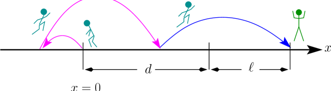
Figure 8: Schematic of the leapover problem: the random walker starts at $x=0$ and after a number of jumps crosses the point $x=d$, overshooting it by a distance $\ell$. For narrow jump length distributions, each jump is so small that crossing of the point $d$ is equal to arriving at this point.

Using a general theorem for the first passage times and leapovers for homogeneous processes with independent increments, leapover properties for completely symmetric and fully asymmetric (one-sided) LFs are derived in leapover , the general case is considered in leapover1 . The basic results are as follows. For the completely symmetric LF with index $\mu$, the distribution of first passage leapover lengths $\ell$ for a particle originally released a distance $d$ away from the boundary reads (in scaled units)

$$p_{l}(\ell)=\frac{\sin(\pi\mu/2)}{\pi}\frac{d^{\mu/2}}{\ell^{\mu/2}(d+\ell)}.$$ (53)

The validity of this result is confirmed by extensive simulations, for more details refer to leapover ; leapover1 ; kochekla . Note that $p_{l}$ is normalised. In the limit $\mu\to 2$, $p_{l}$ tends to zero if $\ell\neq 0$ and to infinity at $\ell=0$ corresponding to the absence of leapovers in the Gaussian continuum limit. However, for $0<\mu<2$ the leapover PDF follows an asymptotic power-law with index $\mu/2$, and is thus broader than the original jump length PDF $\lambda(x)$ with index $\mu$. This is a remarkable finding: while $\lambda$ for $1<\mu<2$ has a finite characteristic length $\langle|x|\rangle$, this always diverges for $p_{l}(\ell)$ irrespective of $\mu$.

In contrast, the result for completely asymmetric LFs has the form Eliazar and Klafter (2003); leapover

$$p_{l}(q)=\langle e^{-q\ell}\rangle=\frac{\sin(\pi\mu)}{\pi}\int_{0}^{\infty}e^{-q\ell}\frac{x^{\mu}}{\ell^{\mu}(x+\ell)},$$ (54)

leading to the leapover PDF

$$p_{l}(\ell)=\frac{\sin(\pi\mu)}{\pi}\frac{d^{\mu}}{\ell^{\mu}(d+\ell)},$$ (55)

which corresponds to the result obtained in Refs. iddoyossi ; tal from a different method. Thus, for the one-sided LF, the scaling of the leapover is exactly the same as for the jump length distribution, namely, with exponent $\mu$. Again, this result compares favourably with simulations leapover ; leapover1 .

III.6 Kramers problem for Lévy flights

Many physical and chemical problems are related to the thermal fluctuations driven crossing of an energetic barrier, such as dissociation of molecules, nucleation processes, or the escape from an external, confining potential of finite height haenggi . A particular example of barrier crossing in a double-well potential driven by Lévy noise was proposed for a long time series of paleoclimatic data Ditlevsen (1999). Further cases where the crossing of a potential barrier driven by Lévy noise is of interest is in the theory of plasma devices Chechkin et al. (2002), among others Metzler and Klafter (2004).

To investigate the detailed behaviour of barrier crossing under the influence of external Lévy noise, we choose the rather generic double well shape

$$V(x)=-\frac{a}{2}x^{2}+\frac{b}{4}x^{4}.$$ (56)

Integrating the Langevin equation (26) with white Lévy noise, we find an exponential decay of the survival density in the initial well:

$$p(t)=\frac{1}{T_{c}}\exp\left(-\frac{t}{T_{c}}\right),$$ (57)

as demonstrated in Fig. 9. Lévy flight processes being Markovian, this is not surprising, since the mode relaxation is exponential Metzler and Klafter (2000, 2004). More interesting is the question how the mean escape time $T_{c}$ behaves as function of the characteristic noise parameters $D$ and $\mu$. While in the regular Kramers problem with Gaussian driving noise the Arrhenius-type activation $T_{c}=C\exp(h/D)$ is followed, where $h$ is the barrier height, and the prefactor $C$ includes details of the potential, in the case of Lévy noise, a power-law form

$$T_{c}(\mu,D)=\frac{C(\mu)}{\left(K^{(\mu)}\right)^{\mu(\mu)}}$$ (58)

was assumed Chechkin et al. (2005). Detailed investigations Chechkin et al. (2007) show that the scaling exponent $\mu(\mu)=1$ for all $\mu$ strictly smaller than 2. As already proposed in Ref. Ditlevsen (1999a) and derived in Imkeller and Pavlyukevich (2006) in a somewhat different model, this means that, apart from a prefactor, the Lévy flight is insensitive to the external potential for the barrier crossing, as confirmed by simulations Chechkin et al. (2007). Note that in comparison to Ref. Chechkin et al. (2005), also values of $\mu$ in the range $(0,1)$ are included. For large values of $D$, deviations from the scaling are observed: eventually it will only take a single jump to cross the barrier when $D\to\infty$. Detailed studies show indeed that eventually the unit time step is reached, i.e., $T_{c}\to 1$.

Figure 9: Probability density function $p(t)$ of barrier crossing times for $\mu=1.0$ and $D=10^{-2.5}\approx 0.00316$. The dashed line is a fit to equation (57) with MCT $T_{c}=1057.8\pm 17.7$.

III.7 More on the ”pathology”

Despite their mathematical foundation due to the generalised central limit theorem and their broad use in the sciences and beyond as description for statistical quantities, and despite the existence of systems (for instance, the diffusion on a polymer in chemical space mediated by jumps where the polymer loops back on itself Sokolov et al. (1997); Brockmann and Geisel (2003); Lomholt et al. (2005)), the divergence of the fluctuations of Lévy processes is sometimes considered a pathology. This was already put forward by West and Seshadri West and Seshadri (1982), who pointed out that a Lévy flight in velocity space would be equivalent to a diverging kinetic energy. Here, we show that higher order dissipation effects lead to natural cutoffs in Lévy processes.

At higher velocities the friction experienced by a moving body starts to depend on the velocity itself Bogoliubov and Mitropolsky (1961). Such non-linear friction is known from the classical Riccati equation $Mdv(t)/dt=Mg-Kv(t)^{2}$ for the fall of a particle of mass $M$ in a gravitational field with acceleration $g$ Davis (1962), or autonomous oscillatory systems with a friction that is non-linear in the velocity Bogoliubov and Mitropolsky (1961); andronov . The occurrence of a non-constant friction coefficient $\gamma(V)$ leading to a non-linear dissipative force $-\gamma(V)V$ was highlighted in Klimontovich’s theory of non-linear Brownian motion klimontovich . It is therefore natural that higher order, non-linear friction terms also occur in the case of Lévy processes.

We consider the velocity-dependent dissipative non-linear form (necessarily an even function) Chechkin et al. (2005a)

$$\gamma(V)=\gamma_{0}+\gamma_{2}V^{2}+\ldots+\gamma_{2N}V^{2N}\quad\therefore\gamma_{2N}>0$$ (59)

for the friction coefficient of the Lévy flight in velocity space as governed by the Langevin equation

$$dV(t)+\gamma(V)V(t)dt=dL(t)$$ (60)

with the constant friction $\gamma_{0}=\gamma(0)$. $L(t)$ is the $\mu$-stable Lévy noise defined in terms of a characteristic function $p^{*}(\omega,t)=\mathscr{F}\{p(L,t)\}\equiv\int_{-\infty}^{\infty}p(L,t)\exp\left(i\omega L\right)dL$ of the form $p^{*}(\omega,t)=\exp\left(-D|\omega|^{\mu}t\right)$ Lévy (1954); Samorodnitsky and Taqqu (1994); uchaikin , where $D$ of dimension ${\rm cm}^{\mu}/{\rm sec}$ is the generalised diffusion constant. This is equivalent to the fractional Fokker Planck equation Fogedby (1998); fogedby1 ; Chechkin et al. (2002, 2004); Metzler and Klafter (2000, 2004)

$$\frac{\partial P(V,t)}{\partial t}=\frac{\partial}{\partial V}\Big{(}V\gamma(V)P\Big{)}+D\frac{\partial^{\mu}P}{\partial|V|^{\mu}}.$$ (61)

As we showed in Sec. III.3.2 by the example of the Lévy flights in position space, the presence of the first higher order correction, $\gamma_{2}V^{2}$ in the friction coefficient $\gamma(V)$ rectifies the Lévy motion such that the asymptotic power-law becomes steeper and the variance finite. When even higher order corrections are taken into consideration, also higher order moments become finite. We show an example in Fig. 10 for the second moment.

Figure 10: Variance $\langle V^{2}(t)\rangle$ as function of time $t$, with the quartic term set to zero, $\gamma_{4}=0$ and $\gamma_{0}=1.0$ for all cases. The variance is finite for the cases $\mu=2.0,\gamma_{2}=0.0$; $\mu=1.2,\gamma_{2}=0.1$; $\mu=1.5,\gamma_{2}=0.1$; and $\mu=1.8,\gamma_{2}=0.1$. These correspond to the left ordinate. For the case $\mu=1.2,\gamma_{2}=0.0$, the variance diverges, strong fluctuations are visible; note the large values of this curve corresponding to the right ordinate.

The effect on the velocity distribution of the process defined by Eqs. (60) and (61) for higher order corrections are demonstrated in Fig. 11 for the stationary limit, $P_{\mathrm{st}}(V)=\lim_{t\to\infty}P(V,t)$: while for smaller $V$ the character of the original Lévy stable behaviour is preserved (the original power-law behaviour, that is, persists to intermediately large $V$), for even larger $V$ the corrections due to the dissipative non-linearity are visible in the transition(s) to steeper slope(s).

Figure 11: Stationary PDF $P_{\mathrm{st}}(V)$ for $\gamma_{0}=1.0$ and (i) $\gamma_{2}=0.0001$ and $\gamma_{4}=0$; and (ii) $\gamma_{2}=0$ and $\gamma_{4}=0.000001$; with $\mu=1.0$. The lines indicate the slopes $-1$, $-3$, and $-5$.

These dissipative non-linearities remove the divergence of the kinetic energy from the measurable subsystem of the random walker. In the ideal mathematical language, the surrounding bath provides an infinite amount of energy through the Lévy noise, and the coupling via the non-linear friction dissipates an infinite amount of energy into the bath, and thereby introduces a natural cutoff in the kinetic energy distribution of the random walker subsystem. Physically, such divergencies are not expected, but correspond to the limiting procedure of large numbers in probability theory. We showed that both statements can be reconciled, and that Lévy processes are indeed physical.

Also Gaussian continuum diffusion exhibits non-physical features, possibly the most prominent being the infinite propagation speed inherent of the parabolic nature of the diffusion equation: even at very short times after system preparation in, say, a state $P(x,0)=\delta(x)$, there has already arrived a finite portion of probability at large $x$. This problem can be corrected by changing from the diffusion to the Cattaneo (telegrapher’s) equation. Still, for most purposes, the uncorrected diffusion equation is used. Similarly, one often uses natural boundary conditions even though the system under consideration is finite, since one might not be interested in the behaviour at times when a significant portion of probability has reached the boundaries. In a similar sense, we showed that ”somewhere out in the wings” Lévy flights are naturally cut off by dissipative non-linear effects. However, instead of introducing artificial cutoffs, knowing that for all purposes Lévy flights are a good quantitative description and therefore meaningful, we use ”pure” Lévy stable laws in physical models.

III.8 Bi-fractional transport equations

The coexistence of long-tailed forms for both jump length and waiting time PDFs was investigated within the CTRW approach in Ref. zuklaa , discussing in detail the laminar-localised phases in chaotic dynamics. In the framework of fractional transport equations, the combination of the waiting time PDF $\psi(t)\sim t^{-1-\alpha}$ ($0<\alpha<1$) and jump length PDF $\lambda(x)\sim|x|^{-1-\mu}$ leads to a dynamical equation with fractional derivatives in respect to both time and space luchko ; mainardi ; Metzler and Nonnenmacher (2002); weno :

$$\frac{\partial}{\partial t}P(x,t)=K_{\alpha}^{(\mu)}\,{}_{0}D_{t}^{1-\alpha}\frac{\partial^{\mu}}{\partial|x|^{\mu}}P(x,t).$$ (62)

As long as the condition $1\leq\alpha\leq\mu\leq 2$ is met, both exponents can be chosen within the entire range mainardi . For $\mu=2$, in particular, this equation covers both sub- and superdiffusion up to ballistic motion, the latter corresponding to the wave equation abm . A closed form solution of Eq. (62) can be found in terms of Fox’s $H$-functions, see Ref. Metzler and Nonnenmacher (2002), where also some special cases permitting elementary solutions are considered. Bi-fractional diffusion equations were also discussed in Refs. barkaicp ; saichev1 ; baeumer ; hughes1 ; gorenflo2 ; uchaikin2 . A bi-fractional Fokker-Planck equation with a power-law dependence $\propto|x|^{-\theta}$ ($\theta\in\mathbb{R}$) of the diffusion coefficient was studied in Refs. fa ; lenzi .

III.9 Lévy walks

Lévy walks correspond to the spatiotemporally coupled version of continuous time random walks. The waiting time and jump length PDFs, that is, are no longer decoupled but appear as conditional in the form $\psi(x,t)\equiv\lambda(x)p(t|x)$ (or $\psi(t)\tilde{p}(x|t)$) Klafter et al. (1987). In particular, through the coupling $p(t|x)=\frac{1}{2}\delta\left(|x|-vt^{\nu}\right)$, one introduces a generalised velocity $v$, which penalises long jumps such that the overall process, the Lévy walk, attains a finite variance and a PDF with two spiky fronts successively exploring space Zumofen and Klafter (1993); Klafter and Zumofen (1994). Thus, Lévy walks have similar properties to generalised Cattaneo/telegraphers’ equation-type models come ; Metzler and Compte (2000a); meno . As we here focus on the properties of transport processes governed by the Langevin equation under Lévy noise, we only briefly introduce Lévy walks.

On the basis of fractional equations, formulations were obtained for the description of Lévy walks in the presence of non-trivial external force fields, with the same restriction to lower order moments in respect to an Lévy walk process basil ; meso . Recently, however, a coupled fractional equations was reported some , which describes a force-free Lévy walk exactly. Thus, it was shown that the fractional version of the material derivative $\partial/\partial t\pm\partial/\partial x$,

$$d_{\pm}^{\beta}P(x,t)\equiv\,_{0}D_{t}^{\beta}P(x\pm t,t),$$ (63)

defined in Fourier-Laplace space through

$$\mathscr{F}\left\{\mathscr{L}\left\{d_{\pm}^{\beta}f(x,t);u\right\};k\right\}\equiv(u\pm ik)^{\beta}f(k,u)$$ (64)

($\mathscr{F}$ acts on $x$ and $\mathscr{L}$ on $t$) replaces the uncoupled fractional time operators, see also the detailed discussion of Lévy walk processes in Ref. Zumofen and Klafter (1993). Although one may argue for certain forms some , there is so far no derivation for the incorporation of general external force fields in the coupled formalism. We note that a very similar fractional approach to Lévy walks was suggested in Ref. meerschaert .

IV Subdiffusion and the fractional Fokker-Planck equation

IV.1 Physical foundation of subdiffusion

The stochastic motion of a Brownian particle of mass $m$ is described by the Langevin equation langevin ; van Kampen (1981); chandrasekhar

$$m\frac{d^{2}x}{dt^{2}}=-m\eta_{1}v+F(x)+m\mathit{\Gamma}(t),\,\,v=\frac{dx}{dt},$$ (65)

where $F(x)$ is an external force field, and $\eta_{1}$ is the friction coefficient. The erroneous bombardment through the surrounding bath molecules is described by the fluctuating noise $\mathit{\Gamma}(t)$. To properly describe Brownian motion, $\mathit{\Gamma}(t)$ has to be chosen $\delta$-correlated (white) and Gaussian distributed. This is, the time averages of $\mathit{\Gamma}(t)$ are: $\overline{\mathit{\Gamma}(t)}=0$, and $\overline{\mathit{\Gamma}(t)\mathit{\Gamma}(t^{\prime})}=D\delta(t-t^{\prime})$, where $D$ is the noise strength. After averaging of the fluctuations, the velocity moments become chandrasekhar

$$\langle\Delta v\rangle=\left(\eta v-\frac{F(x)}{m}\right)\Delta t,\,\,\langle(\Delta v)^{2}\rangle=\frac{2\eta k_{B}T}{m}\Delta t+\mathcal{O}\left([\Delta t]^{2}\right).$$ (66)

Both are proportional to $\Delta t$. For regular Brownian motion, these increments are used as expansion coefficients in the Chapman-Kolmogorov equation chandrasekhar .

Subdiffusion now comes about through a so-called trapping scenario. Trapping describes the occasional immobilisation of the test particle for a waiting time distributed according to the distribution $\psi(t)$. Here we assume that the particle leaves the trap with the same velocity it had prior to immobilisation (this condition can be relaxed). In between trapping events, the particle is assumed to follow the regular Langevin equation such that each motion event on average lasts for a mean time $\tau^{*}$. Choosing $\psi(t)$ with a finite characteristic waiting time one can show that this trapping scenario indeed preserves Brownian motion. However, once the characteristic waiting time diverges, it can be shown by application of the generalised central limit theorem that the occurrence of a large number of trapping events leads to subdiffusion and the fractional Klein-Kramers equation for the joint PDF $P(x,v,t)$ gcke ; meklacke ; meklacke1 . Integrating out the velocity coordinate, the fractional Fokker-Planck equation emerges for the PDF $P(x,t)$:

$$\frac{\partial P(x,t)}{\partial t}=\,_{0}D_{t}^{1-\alpha}\frac{\partial}{\partial x}\left(-\frac{F(x)}{m\eta_{\alpha}}+K_{\alpha}\frac{\partial}{\partial x}\right)P(x,t).$$ (67)

In mathematical terms the trapping scenario corresponds to a subordination principle: Trapping events cause a transformation of the internal step time of the random walk to a different observation time, corresponding to the relation

$$P(x,t)=\int_{0}^{\infty}\mathscr{E}_{\alpha}(s,t)P_{1}(x,s)ds,$$ (68)

where $P_{1}(x,t)$ is the solution of the regular Brownian Fokker-Planck equation with $\alpha=1$. Explicit forms of the kernel $\mathscr{E}_{\alpha}(s,t)$ are known in terms of Fox’ $H$-function Metzler and Klafter (2000). In the Laplace domain, the kernel $\mathscr{E}_{\alpha}(s,t)$ has the comparatively simple form

$$\mathscr{E}_{\alpha}(s,u)\frac{\eta_{\alpha}}{\eta_{1}u^{1-\alpha}}\exp\left(-\frac{\eta_{\alpha}}{\eta_{1}}u^{\alpha}s\right).$$ (69)

Note that this transformation guarantees the existence and positivity of the solution $P(x,t)$ of the fractional Fokker-Planck equation if only the corresponding Brownian problem possesses a well-defined solution. We note that recently an alternative approach to continuous time random walk subdiffusion in terms of $\delta$-noise spike trains was presented saichev .

IV.2 Linear response and fluctuation-dissipation relation

From the fractional Fokker-Planck equation (67) it is straightforward to prove that in the presence of a constant field $F_{0}$ the linear response relation

$$\langle x(t)\rangle_{F_{0}}=\frac{k_{B}T}{2}\langle x^{2}(t)\rangle_{F=0}$$ (70)

is fulfilled Metzler et al. (1999); Metzler and Klafter (2000). This is due to the fact that the waiting time distribution $\psi(t)$ is independent of the force. Given the comparatively large traps required to create the long-tailed form of $\psi(t)$, this assumption appears reasonable for not too large $F_{0}$. Experimentally, the linear response relation (70) was verified schiff .

The stationary solution of the fractional Fokker-Planck equation (67) is the standard Boltzmann-Gibbs equilibrium, $\lim_{t\to\infty}P(x,t)=\mathscr{N}\exp\left\{-V(x)/[k_{B}T]\right\}$, where $\mathscr{N}$ is a normalisation constant Metzler et al. (1999). This result is immediately obvious from the picture of subordination, that changes the temporal spacing of events but preserves the causal mode relaxation. As $F(x)=-V^{\prime}(x)$, from the stationary solution of Eq. (67) by comparison with the Boltzmann-Gibbs form one recovers the generalised Einstein-Stokes relation Metzler et al. (1999)

$$K_{\alpha}=\frac{k_{B}T}{m\eta_{\alpha}},$$ (71)

reflecting the preservation of the fluctuation-dissipation relation for the subdiffusion process. An experimental verification of this relation was reported by amblard .

IV.3 Propagator

In absence of an external force, the fractional diffusion equation is solved by Fox’ $H$-function Metzler and Klafter (2000),

$$W(x,t)=\frac{1}{\sqrt{4K_{\alpha}t^{\alpha}}}H^{1,0}_{1,1}\left[\frac{|x|}{\sqrt{K_{\alpha}t^{\alpha}}}\left|\begin{array}[]{l}\left(1-\frac{\alpha}{2},\frac{\alpha}{2}\right)\\ (0,1)\end{array}\right.\right],$$ (72)

an equivalent form to the original solution by schneider . Its series expansion reads Metzler and Klafter (2000)

$$W(x,t)=\frac{1}{\sqrt{4K_{\alpha}t^{\alpha}}}\sum_{n=0}^{\infty}\frac{(-1)^{n}}{n!\Gamma(1-\alpha[n+1]/2)}\left(\frac{x^{2}}{K_{\alpha}t^{\alpha}}\right)^{n/2},$$ (73)

and asymptotically reaches the stretched Gaussian form

$$W(x,t) \sim \frac{1}{\sqrt{4\pi K_{\alpha}t^{\alpha}}}\sqrt{\frac{1}{2-\alpha}}\left(\frac{2}{\alpha}\right)^{(1-\alpha)/(2-\alpha)}\left(\frac{|x|}{\sqrt{K_{\alpha}t^{\alpha}}}\right)^{-(1-\alpha)/(2-\alpha)}$$ (74)

$$\times\exp\left(-\frac{2-\alpha}{2}\left(\frac{\alpha}{2}\right)^{\alpha/(2-\alpha)}\left[\frac{|x|}{\sqrt{K_{\alpha}t^{\alpha}}}\right]^{1/(1-\alpha/2)}\right).$$

valid for $|x|\gg\sqrt{K_{\alpha}t^{\alpha}}$. The latter corresponds to the known result from continuous time random walk theory Zumofen and Klafter (1993); Klafter and Zumofen (1994). The $H$-function simplifies if the exponent $\alpha$ is a rational number. For instance, for $\alpha=1/2$, it can be rewritten in terms of the Meijer $G$-function

$$P(x,t)=\frac{1}{\sqrt{8\pi^{3}K_{1/2}t^{1/2}}}G^{3,0}_{0,3}\left[\left(\frac{x^{2}}{16K_{1/2}t^{1/2}}\right)^{2}\left|\begin{array}[]{l}\rule[4.33601pt]{28.90755pt}{0.72229pt}\\ 0,\frac{1}{4},\frac{1}{2}\end{array}\right.\right],$$ (75)

that is known in symbolic mathematics packages such as Mathematica. Using this representation in Fig. 12 we show the subdiffusive propagator with its pronounced cusps at the site of the initial condition, in comparison to the smooth Gaussian propagator of Brownian motion.

Figure 12: Propagator $P(x,t)$ of the fractional diffusion equation with $\alpha=1/2$ (left) and the normal diffusion equation (right) for consecutive times.

IV.4 Boundary value and first passage time problems

In the presence of reflecting, absorbing, or mixed, boundary conditions, the narrow jump length distribution of subdiffusive processes makes it possible to use analogous techniques to calculate the propagator as known from normal diffusion. Thus, separation into eigenmodes or the method of images can be applied, the only difference entering through the time-dependence of the modes. A very convenient way is to employ the Brownian result for a given geometry, and subordinate that result to obtain the behaviour for a subdiffusing particle, according to Eq. (68).

In the presence of an absorbing boundary an important quantity characterising the dynamics of the system is the survival probability

$$\mathscr{S}_{\alpha}(t)=\int_{\mathbb{D}}\mathscr{P}(x,t)dx,$$ (76)

where $\mathbb{D}$ denotes the interval over which $\mathscr{P}(x,t)$ is defined. The initial value of the survival probability is $\mathscr{S}_{\alpha}(0)=1$, and it decays to zero for long times. From $\mathscr{S}_{\alpha}(t)$, we can define the first passage time density

$$p_{\alpha}(t)=-\frac{d}{dt}\mathscr{S}_{\alpha}(t).$$ (77)

The mean first passage time is

$$\mathcal{T}=\int_{0}^{\infty}p_{\alpha}(t)tdt.$$ (78)

Note that from Eqs. (77) and (68), we obtain the relation

$$p_{\alpha}(u)=p_{1}\left(u^{\alpha}\right)$$ (79)

between the subdiffusive and Brownian results in Laplace space. Thus, these are connected by a relation similar to the subordination (68), with kernel $\exp\left(-su^{\alpha}\right)$ instead of $\mathscr{E}_{\alpha}(s,u)$ Metzler and Klafter (2004); yossibj .

For the three most prominent cases of first passage time problems, we obtain the following subdiffusive generalisations:

(i) For subdiffusion in the semi-infinite domain with an absorbing wall at the origin and initial condition $P(x,0)=\delta(x-x_{0})$ it was found that Metzler and Klafter (2000b)

$$p(t)\sim\frac{x_{0}}{|\Gamma(-\alpha/2)|K_{\alpha}^{1/2}}t^{-1-\alpha/2},$$ (80)

i.e., the decay becomes a flatter power-law than in the Markovian case where $p(t)\sim t^{-3/2}$.

(ii) Subdiffusion in the semi-infinite domain in the presence of an external bias $V$ falls off faster, but still in power-law manner barkai ; yossibj ; grl :

$$p(t)\sim t^{-1-\alpha}.$$ (81)

In strong contrast to the biased Brownian case, we now end up with a process whose characteristic time scale diverges. This is exactly the mirror of the multiple trapping model, i.e., the classical motion events become repeatedly interrupted such that the immobilisation time dominates the process. In contrast, for $\alpha=1$ the result

$$p_{1}(t)=\frac{x_{0}}{\sqrt{4\pi K_{\alpha}t^{3}}}\exp\left(-\frac{(x_{0}-Vt)^{2}}{4Kt}\right)$$ (82)

is valid, producing the classical form $\mathcal{T}=x_{0}/V$ for the mean first passage time.

(iii) Subdiffusion in a finite box Metzler and Klafter (2000b):

$$p(t)\sim t^{-1-\alpha},$$ (83)

i.e., this process leads to the same scaling behaviour for longer times as found for the biased semi-infinite case (ii).

The latter two results should be compared to the classical Scher-Montroll finding for the first passage time density of biased motion in a finite system of size $L$ with absorbing boundary condition. In that case, the first passage time density exhibits two power-laws

$$p(t)\sim\left\{\begin{array}[]{ll}t^{\alpha-1},&t<\tau\\ t^{-1-\alpha},&t>\tau\end{array}\right.$$ (84)

the sum of whose exponents equals $-2$ pfister ; pfister ; Montroll and Scher (1973); grl . Here, $\tau$ is a system size dependent time scale pfister .

IV.5 Fractional Ornstein-Uhlenbeck process

The Ornstein-Uhlenbeck process corresponds to the motion in an harmonic potential $V(x)=\frac{1}{2}m\omega^{2}x^{2}$ giving rise to the restoring force field $F(x)=-m\omega^{2}x$, i.e., to the dynamical equation

$$\frac{\partial}{\partial t}P(x,t)=\,_{0}D_{t}^{1-\alpha}\left(\frac{\partial}{\partial x}\frac{\omega^{2}x}{\eta_{\alpha}}+K_{\alpha}\frac{\partial^{2}}{\partial x^{2}}\right)P(x,t).$$ (85)

From separation of variables, and the definition of the Hermite polynomials abramowitz , one finds the series solution for the fractional Fokker-Planck equation with the Ornstein-Uhlenbeck potential Metzler et al. (1999); Metzler and Klafter (2000),

$$P(x,t)=\sqrt{\frac{m\omega^{2}}{2\pi k_{B}T}} \sum_{n=0}^{\infty}\frac{1}{2^{n}n!}E_{\alpha}\left(-\frac{n\omega^{2}t^{\alpha}}{\eta_{\alpha}}\right)H_{n}\left(\frac{\sqrt{m}\omega x_{0}}{\sqrt{2k_{B}T}}\right)$$ (86)

$$\times H_{n}\left(\frac{\sqrt{m}\omega x}{\sqrt{2k_{B}T}}\right)\exp\left(-\frac{m\omega^{2}x^{2}}{2k_{B}T}\right)$$

plotted in Fig. 13.

Figure 13: Time evolution of the PDF of the fractional Ornstein-Uhlenbeck process ($\alpha=1/2$). The initial condition was chosen as $\delta(x-1)$. Note the strongly persistent cusp at the location of the initial peak. Dimensionless times: 0.02, 0.2, 2. The dashed line corresponds to the Boltzmann equilibrium.

Individual spatial eigenmodes follow the ordinary Hermite polynomials of increasing order, while their temporal relaxation is of Mittag-Leffler form, with decreasing internal time scale $\left(\eta_{\alpha}/[n\omega^{2}]\right)^{1/\alpha}$. Numerically, the solution (86) is somewhat cumbersome to treat. In order to plot the PDF $P(x,t)$ in Fig. 13, it is preferable to use the closed form solution (we use dimensionless variables)

$$P(x,t)=\frac{1}{\sqrt{2\pi\left(1-e^{-2t}\right)}}\exp\left(-\frac{\left(x-x_{0}e^{-t}\right)^{2}}{2\left(1-e^{-2t}\right)}\right)$$ (87)

of the Brownian case, and the transformation (68) to construct the fractional analogue.

Figure 14: Time evolution of the PDF of the fractional Ornstein-Uhlenbeck process with superposed constant force of dimensionless strength $V=-4$ ($\alpha=1/2$). The initial condition was chosen as $\delta(x-4)$. Dimensionless times: 0.02, 0.2, 2. The dashed lines corresponds to the Brownian solution at times 0.5 and 50 (in essence, the stationary state). Again, note the cusps due to the initial condition, causing a strongly asymmetric shape of the PDF in contrast to the Gaussian nature of the Brownian counterpart.

Figure 15: First ($x_{0}=2$, dashed line) and second ($x_{0}=0$, full line) moment of the fractional Ornstein-Uhlenbeck process ($\alpha=1/2$), in comparison to the Brownian case. $\log_{10}$$-$$\log_{10}$ scale. The dotted straight lines show the initial (sub)diffusive behaviour with slopes 1/2 and 1, in the special case $x_{0}=0$ chosen for the second moment.

Fig. 13 shows the distinct cusps at the position of the initial condition at $x_{0}=1$. The relaxation to the final Gaussian Gibbs-Boltzmann PDF can be seen from the sequence of three consecutive times. Only at stationarity, the cusp gives way to the smooth Gaussian shape of the equilibrium PDF. By adding an additional linear drift $V$ to the harmonic restoring force, the drift term in the FFPE (67) changes to $-\partial(x-V)P(x,t)/\partial x$, and the exponential in expression (87) takes on the form $\exp\left(-\left[x-V-(x_{0}-V)e^{-t}\right]/\left[2\left(1-e^{-2t}\right)\right]\right)$. As displayed in Fig. 14, the strong persistence of the initial condition causes a highly asymmetric shape of the PDF, whereas the Brownian solution shown in dashed lines retains its symmetric Gaussian profile.

Let us finally address the moments of the fractional Ornstein-Uhlenbeck process, Eq. (86). These can be readily obtained either from the Brownian result with the integral transformation (68), or from integration $\int dxx^{n}\cdot$ of the FFPE (67). For the first and second moments one obtains:

$$\langle x(t)\rangle=x_{0}E_{\alpha}\left(-\frac{\omega^{2}t^{\alpha}}{\eta_{\alpha}}\right)$$ (88)

and

$$\langle x(t)^{2}\rangle=x_{\rm th}^{2}+\left(x_{0}^{2}-x_{\rm th}^{2}\right)E_{\alpha}\left(-\frac{2\omega^{2}t^{\alpha}}{\eta_{\alpha}}\right),$$ (89)

respectively. The first moment starts off at the initial position, $x_{0}$, and then falls off in a Mittag-Leffler pattern, reaching the terminal inverse power-law $\sim t^{-\alpha}$. The second moment turns from the initial value $x_{0}^{2}$ to the thermal value $x_{\rm th}^{2}=k_{B}T/(m\omega^{2})$. In the special case $x_{0}=0$, the second moment measures initial force-free diffusion due to the initial exploration of the flat apex of the potential. We graph the two moments in Fig. 15 in comparison to their Brownian counterparts.

V Future directions

Anomalous diffusion is becoming widely recognised in a variety of fields. Apart from the anomalous spreading of tracers and the consequences for the propagator, additional questions such as ageing and weak ergodicity breaking become important for the understanding of experiments and their modelling on complex systems. At the same time, the theory of anomalous processes is expanding. For instance, regarding questions on the weak ergodicity breaking, the calculation of multipoint moments or the correct introduction of cutoffs are currently being worked on, to complete the world Beyond Brownian Motion physicstoday .

VI Bibliography

Books and Reviews

References

- (1) Abramowitz M, Stegun I (1972) Handbook of Mathematical Functions. Dover, New York, NY
- (2) Andronow AA, Chaikin CE, Lefschetz S (1949) Theory of oscillations. University Press, Princeton, NJ
- Bogoliubov and Mitropolsky (1961) Bogoliubov NN, Mitropolsky YA (1961) Asymptotic methods in the theory of non-linear oscillations. Hindustan Publ. Corp., Delhi (distr. by Gordon & Breach, New York, NY
- (4) Bouchaud JP, Georges A (1990) Anomalous diffusion in disordered media: statistical mechanisms, models and physical applications. Physics Reports 195: 127-293
- (5) Carus TL (1975) De rerum natura (50 BCE): On the nature of things. Harvard University Press, Cambridge, MA
- (6) Chandrasekhar S (1943) Stochastic problems in physics and astronomy. Reviews of Modern Physics 15: 1-89
- (7) Chechkin AV, Gonchar VYu, Klafter J, Metzler R (2006) Fundamentals of Lévy flight processes. Advances in Chemical Physics 133B: 439-496
- Davis (1962) Davis H (1962) Introduction to nonlinear differential and integral equations. Dover Publications, Inc., New York, NY
- Feller (1971) Feller W (1971) An Introduction to Probability Theory and its Applications, Vol. 2. Wiley, New York, NY
- Frisch and Frisch (1995) Frisch U, Frisch H (1995) Universality of escape from a half space for symmetrical random walks. In: Shlesinger MF, Zaslavsky GM, Frisch U (eds) Lévy flights and related topics in physics. Lecture Notes in Physics, Vol. 450: 262-268. Springer-Verlag, Berlin
- Gnedenko and Kolmogorov (1954) Gnedenko BV, Kolmogorov AN (1954) Limit Distributions for Sums of Random Variables. Addison-Wesley, Reading, MA
- (12) Hänggi P, Talkner P, Borkovec M (1990) Reaction-rate theory - 50 years after Kramers. Reviews of Modern Physics 62: 251-341
- Hughes (1995) Hughes BD (1995) Random Walks and Random Environments, Vol. 1. Oxford University Press, Oxford
- (14) Ingenhousz J (1785) Nouvelles expériences et observations sur divers objets de physique. T. Barrois le jeune, Paris
- (15) Klimontovich YuL (1992) Turbulent motion and the structure of chaos: a new approach to the statistical theory of open systems. Kluwer, Dordrecht
- Lévy (1954) Lévy P (1954) Théorie de l’addition des variables aléatoires. Gauthier-Villars, Paris
- Metzler and Klafter (2000) Metzler R, Klafter J (2000) The random walk’s guide to anomalous diffusion: a fractional dynamics approach. Physics Reports 339: 1-77
- Metzler and Klafter (2004) Metzler R, Klafter J (2004) The restaurant at the end of the random walk: recent developments in the description of anomalous transport by fractional dynamics. Journal of Physics A-Mathematical and General 37: R161-R208
- Montroll and West (1976) Montroll EW, West BJ (1976) In: Montroll EW, Lebowitz JL (eds) Fluctuation phenomena. North-Holland, Amsterdam YOSSI, PLEASE CHECK THE TITLE OF THE CHAPTER AND THE PAGES.
- (20) Oldham KB, Spanier J (1974) The fractional calculus. Academic Press, New York, NY
- Podlubny (1998) Podlubny I (1998) Fractional differential equations. Academic Press, San Diego, CA
- Redner (2001) Redner S (2001) A guide to first-passage processes. Cambridge University Press, Cambridge, UK
- Risken (1989) Risken H (1989) The Fokker-Planck equation. Springer-Verlag, Berlin
- Samko et al. (1993) Samko SG, Kilbas AA, Marichev OI. (1993) Fractional Integrals and Derivatives, Theory and Applications. Gordon and Breach, New York, NY
- Samorodnitsky and Taqqu (1994) Samorodnitsky G, Taqqu MS (1994) Stable non-gaussian random processes: Stochastic models with infinite variance. Chapman and Hall, New York, NY
- (26) Uchaikin VV, Zolotarev VM (1999) Chance and stability. Stable distributions and their applications. VSP, Utrecht
- van Kampen (1981) van Kampen NG (1981) Stochastic Processes in Physics and Chemistry. North-Holland, Amsterdam
- Weiss (1994) Weiss GH (1994) Aspects and Applications of the Random Walk. North-Holland, Amsterdam
-
(29)
Zaslavsky GM (2002) Chaos, fractional kinetics and
anomalous transport. Physics Reports 371: 461-580
Primary literature
- (30) Amblard F, Maggs AC, Yurke B, Pargellis AN, Leibler S (1996) Subdiffusion and anomalous local viscoelasticity in actin networks. Physical Review Letters 77: 4470-4473. Erratum: Physical Review Letters 81: 1136-1136. Reply: Physical Review Letters 81: 1135-1135
- (31) Atkinson RPD, Rhodes CJ, Macdonald DW, Anderson RM (2002) Scale-free dynamics in the movement patterns of jackals. OIKOS 98: 134-140
- (32) Baeumer B, Benson DA, Meerschaert MM (2005) Advection and dispersion in time and space. Physica A-Statistical Mechanics and its Applications 350: 245-262
- (33) Barkai E, Silbey RJ (2000) Fractional Kramers equation. Journal of Physical Chemistry B 104: 3866-3874
- (34) Barkai E (2001) Fractional Fokker-Planck equation, solution, and application. Physical Review E 63: article no. 046118
- (35) Barkai E (2002) CTRW pathways to the fractional diffusion equation. Chemical Physics 284: 13-27
- (36) Barkai E (2006) Aging in subdiffusion generated by a deterministic dynamical system. Physical Review Letters 96: article no. 104101
- (37) Barkai E, Metzler R, Klafter J (2000) From continuous time random walks to the fractional Fokker-Planck equation. Physical Review E 61: 132-138
- (38) Bel G, Barkai E (2006) Weak ergodicity breaking in the continuous-time random walk. Physical Review Letters 94: article no. 240602
- (39) Bouchaud JP (1992) Weak ergodicity breaking and aging in disordered-systems. Journal de Physique 2: 1705-1713
- Brockmann and Geisel (2003) Brockmann D, Geisel T (2003) Particle dispersion on rapidly folding random heteropolymers. Physical Review Letters 91: article no. 048303
- (41) Brown R (1828) A brief account of microscopical observations made in the months of June, July and August, 1827, on the particles contained in the pollen of plants; and on the general existence of active molecules in organic and inorganic bodies. Philosophical Magazine 4: 161-173
- Chechkin et al. (2002) Chechkin AV, Gonchar VYu, Szydlowski M (2002) Fractional kinetics for relaxation and superdiffusion in a magnetic field. Physics of Plasmas 9: 78-88
- Chechkin et al. (2003) Chechkin AV, Klafter J, Gonchar VY, Metzler R, Tanatarov LV (2003) Physical Review E 67: article no. 010102(R)
- Chechkin et al. (2003a) Chechkin AV, Metzler R, Gonchar VY, Klafter J, Tanatarov LV (2003) Journal of Physics A-Mathematical and General 36: L537-L544
- Chechkin et al. (2004) Chechkin AV, Gonchar VY, Klafter J, Metzler R, Tanatarov LV (2004) Journal of Statistical Physics 115: 1505-1535
- Chechkin et al. (2005) Chechkin AV, Gonchar VY, Klafter J, Metzler R (2005) Europhysics Letters 72: 348-354
- Chechkin et al. (2005a) Chechkin AV, Gonchar VY, Klafter J, Metzler R (2005) Physical Review E 72: article no. 010101
- Chechkin et al. (2007) Chechkin AV, Sliusarenko AYu, Metzler R, Klafter J (2007) Barrier crossing driven by Lévy noise: Universality and the role of noise intensity. Physical review E 75: article no. 041101
- (49) Compte A, Metzler R (1997) The generalized Cattaneo equation for the description of anomalous transport processes. Journal of Physics A-Mathematical and General 30: 7277-7289
- Ditlevsen (1999) Ditlevsen PD (1999) Observation of alpha-stable noise induced millennial climate changes from an ice-core record. Geophysical Research Letters 26: 1441-1444
- Ditlevsen (1999a) Ditlevsen PD (1999) Anomalous jumping in a double-well potential. Physical Review E 60: 172-179
- Eliazar and Klafter (2003) Eliazar I, Klafter J (2003) Lévy-driven Langevin systems: Targeted stochasticity. Journal of Statistical Physics 111: 739-768
- (53) Eliazar I, Koren T, Klafter J (2007) Searching circular DNA strands. Journal of Physics-Condensed Matter 19: article no. 065140
- (54) Eliazar I, Klafter J (2004) On the first passage of one-sided Levy motions. Physica A-Statistical Mechanics and its Applications 336: 219-244
- (55) Fa KS, Lenzi EK (2003) Power law diffusion coefficient and anomalous diffusion: Analysis of solutions and first passage time. Physical Review E 67: article no. 061105
- Fogedby (1998) Fogedby HC (1994) Lévy flights in random-environments. Physical Review Letters 73: 2517-2520
- (57) Fogedby HC (1998) Lévy flights in quenched random force fields. Physical Review 58: 1690-1712
- Gittermann (2000) Gitterman M (2000) Mean first passage time for anomalous diffusion. Physical Review E 62: 6065-6070
- (59) Golding I, Cox EC (2006) Physical nature of bacterial cytoplasm. Physical Review Letters 96: article no. 098102
- (60) Fractional diffusion: probability distributions and random walk models. Physica A-Statistical Mechanics and its Applications 305: 106-112
- (61) Gu Q, Schiff EA, Grebner S, Wang F, Schwarz R (1996) Non-Gaussian transport measurements and the Einstein relation in amorphous silicon. Physical Review Letters 76: 3196-3199
- (62) Hughes BD (2002) Anomalous diffusion, stable processes, and generalized functions. Physical Review E 65: article no. 035105
- Imkeller and Pavlyukevich (2006) Imkeller P, Pavlyukevich I (2006) Lévy flights: transitions and meta-stability. Journal of Physics A-Mathematical and General 39: L237-L246
- Jespersen et al. (1999) Jespersen S, Metzler R, Fogedby HC (1999) Lévy flights in external force fields: Langevin and fractional Fokker-Planck equations and their solutions. Physical Review E 59: 2736-2745
- (65) Kappler E (1931) Versuche zur Messung der Avogadro-Loschmidtschen Zahl aus der Brownschen Bewegung einer Drehwaage. Annalen der Physik 11: 233-256
- (66) Katori H, Schlipf S, Walther H (1997) Anomalous dynamics of a single ion in an optical lattice. Physical Review Letters 79: 2221-2224
- Klafter et al. (1987) Klafter J, Blumen A, Shlesinger MF (1987) Stochastic pathway to anomalous diffusion. Physical Review A 35: 3081-3085
- (68) Klafter J, Shlesinger MF, Zumofen G (1996) Beyond Brownian motion. Physics Today 49: 33-39
- Klafter and Zumofen (1994) Klafter J, Zumofen G (1994) Probability distributions for continuous-time random-walks with long tails. Journal of Physical Chemistry 98: 7366-7370
- (70) Koren T, Chechkin AV, Klafter J (2007) On the first passage time and leapover properties of Lévy motion. Physics A 379:10-22
- (71) Koren T, Lomholt MA, Chechkin AV, Klafter J, Metzler R Leapover lengths and first passage time statistics for Lévy flights. In preparation.
- (72) Koren T, Lomholt MA, Chechkin AV, Klafter J, Metzler R Unpublished.
- (73) Langevin P (1908) The theory of brownian movement. Comptes Rendus Hebdomadaires des Seances de l’Academie des Sciences 146: 530-533
- (74) Lenzi EK, Mendes RS, Fa KS, Malacarne LC, da Silva LR (2003) Anomalous diffusion: Fractional Fokker-Planck equation and its solutions. Journal of Mathematical Physics 44: 2179-2185
- (75) Levandowsky M, White BS, Schuster FL (1997) Random movements of soil amebas. Acta Protozoologica 36: 237-248
- Lomholt et al. (2005) Lomholt MA, Ambjornsson T, Metzler R (2005) Optimal target search on a fast-folding polymer chain with volume exchange. Physical Review Letters 95: article no. 260603
- (77) Lomholt MA, Zaid IM, Metzler R (2007) Subdiffusion and weak ergodicity breaking in the presence of a reactive boundary. Physical Review Letters 98: article no. 200603
- (78) Luchko Y, Gorenflo R (1998) Scale-invariant solutions of a partial differential equation of fractional order. Fractional Calculus and Applied Analysis 1: 63-78
- (79) Lutz E (2004) Power-law tail distributions and nonergodicity. Physical Review Letters 93: article no. 190602
- (80) Mainardi F, Luchko Y, Pagnini G (2001) The fundamental solution of the space-time fractional diffusion equation. Fractional Calculus and Applied Analysis 4: 153-192
- (81) Meerschaert MM, Benson DA, Scheffler HP, Becker-Kern P (2002) Governing equations and solutions of anomalous random walk limits. Physical Review E 66: article no. 060102
- (82) Metzler R, Nonnenmacher TF (1998) Fractional diffusion, waiting-time distributions, and Cattaneo-type equations. Physical Review E 57: 6409-6414
- Metzler et al. (1999) Metzler R, Barkai E, Klafter J (1999) Anomalous diffusion and relaxation close to thermal equilibrium: A fractional Fokker-Planck equation approach. Physical Review Letters 82: 3563-3567
- Metzler et al. (1999a) Metzler R, Barkai E, Klafter J (1999) Deriving fractional Fokker-Planck equations from a generalised master equation. Europhysics Letters 46: 431-436
- (85) Metzler R, Klafter J (2000) Accelerating Brownian motion: A fractional dynamics approach to fast diffusion. Europhysics Letters 51: 492-498
- (86) Metzler R (2000) Generalized Chapman-Kolmogorov equation: A unifying approach to the description of anomalous transport in external fields. Physical Review E 62: 6233-6245
- (87) Metzler R, Sokolov IM (2002) Superdiffusive Klein-Kramers equation: Normal and anomalous time evolution and Levy walk moments. Europhysics Letters 58: 482-488
- (88) Metzler R, Klafter J (2003) When translocation dynamics becomes anomalous. Biophysical Journal 85: 2776-2779
- Metzler and Compte (2000a) Metzler R, Compte A (2000) Generalized diffusion-advection schemes and dispersive sedimentation: A fractional approach. Journal of Physical Chemistry B 104: 3858-3865
- Metzler and Klafter (2000b) Metzler R, Klafter J (2000) Boundary value problems for fractional diffusion equations. Physica A-Statistical Mechanics and its Applications 278: 107-125
- Metzler (2001) Metzler R (2001) Non-homogeneous random walks, generalised master equations, fractional Fokker-Planck equations, and the generalised Kramers-Moyal expansion. European Physical Journal B 19: 249-258
- (92) Metzler R, Klafter J (2000) From a generalized Chapman-Kolmogorov equation to the fractional Klein-Kramers equation. Journal of Physical Chemistry B 104: 3851-3857
- (93) Metzler R, Klafter J (2000) Subdiffusive transport close to thermal equilibrium: From the Langevin equation to fractional diffusion. Physical Review E 61: 6308-6311
- Metzler and Nonnenmacher (2002) Metzler R, Nonnenmacher TF (2002) Space- and time-fractional diffusion and wave equations, fractional Fokker-Planck equations, and physical motivation. Chemical Physics 284: 67-90
- (95) Monthus C, Bouchaud JP (1996) Models of traps and glass phenomenology. Journal of Physics A-Mathematical and General 29: 3847-3869
- Montroll and Weiss (1969) Montroll EW, Weiss GH (1965) Random Walks on Lattices. II. Journal of Mathematical Physics 6: 167-181
- (97) Perrin J (1908) Molecular agitation and the brownian movement. Comptes Rendus Hebdomadaires des Seances de l’Academie des Sciences 146: 967-970
- (98) Perrin J (1909) Brownian motion and molecular reality. Annales de Chimie et de Physique 18: 5-114
- (99) Pfister G, Scher H (1978) Dispersive (non-Gaussian) transient transport in disordered solids. Advances in Physics 27: 747-798
- (100) Ramos-Fernandez G, Mateos JL, Miramontes O, Cocho G, Larralde H, Ayala-Orozco B (2004) Lévy walk patterns in the foraging movements of spider monkeys (Ateles geoffroyi). Behavioral Ecology and Sociobiology 55: 223-230
- (101) Priyatinska A, Saichev AI, Woyczynski WA (2005) Models of anomalous diffusion: the subdiffusive case. Physica A 349: 375-420
- (102) Saichev AI, Zaslavsky GM (1997) Fractional kinetic equations: solutions and applications. Chaos 7: 753-764
- Montroll and Scher (1973) Scher H, Montroll EW (1975) Anomalous transit-time dispersion in amorphous solids. Physical Review B 12: 2455-2477
- (104) Scher H, Margolin G, Metzler R, Klafter J, Berkowitz B (2002) The dynamical foundation of fractal stream chemistry: the origin of extremely long retention times. Geophysical Research Letters 29: article no. 1061
- (105) Schneider WR, Wyss W (1989) Fractional diffusion and wave equations. Journal of Mathematical Physics 30: 134-144
- Sokolov et al. (1997) Sokolov IM, Mai J, Blumen A (1997) Paradoxical diffusion in chemical space for nearest-neighbor walks over polymer chains. Physical Review Letters 79: 857-860
- (107) Sokolov IM, Metzler R (2003) Towards deterministic equations for Levy walks: The fractional material derivative. Physical Review E 67: article no. 010101
- Sokolov and Metzler (2004) Sokolov IM, Metzler R (2004) Non-uniqueness of the first passage time density of Levy random processes. Journal of Physics A-Mathematical and General 37: L609-L615
- (109) Sokolov IM, Klafter J, Blumen A (2002) Fractional kinetics. Physics Today 55: 48-54
- Sparre Andersen (1953) Sparre Andersen E (1953) On the fluctuations of sums of random variables. Mathematica Scandinavica 1: 263-285
- Sparre Andersen (1954) Sparre Andersen E (1954) On the fluctuations of sums of random variables II. Mathematica Scandinavica 2: 194-223
- (112) Uchaikin VV (2002) Multidimensional symmetric anomalous diffusion. Chemical Physics 284: 507-520
- (113) Visser AW and Thygesen UH (2003) Random motility of plankton: diffusive and aggregative contributions. Journal of Plankton Research 25: 1157-1168
- (114) Viswanathan GM, Afanasyev V, Buldyrev SV, Murphy EJ, Prince PA, Stanley HE (1996) Lévy flight search patterns of wandering albatrosses. Nature 381: 413-415
- (115) Viswanathan GM, Buldyrev SV, Havlin S, da Luz MGE, Raposo EP, Stanley HE (1999) Optimizing the success of random searches. Nature 401: 911-914
- West and Seshadri (1982) West BJ, Seshadri V (1982) Linear systems with Lévy fluctuations. Physica A 113: 203-216
- (117) West BJ, Grigolini P, Metzler R, Nonnenmacher TF (1997) Fractional diffusion and Levy stable processes. Physical Review E 55: 99-106
- (118) West BJ, Nonnenmacher TF (2001) An ant in a gurge. Physics Letters A 278: 255-259
- (119) Wong IY, Gardel ML, Reichman DR, Weeks ER, Valentine MT, Bausch AR, Weitz DA (2004) Anomalous diffusion probes microstructure dynamics of entangled F-actin networks. Physical Review Letters 92: article no. 178101
- Zumofen and Klafter (1993) Zumofen G, Klafter J (1993) Scale-invariant motion in intermittent chaotic systems. Physical Review E 47: 851-863
- Zumofen and Klafter (1995) Zumofen G, Klafter J (1995) Absorbing boundary in one-dimensional anomalous transport. Physical Review E 51: 2805-2814
- (122) Zumofen G, Klafter J (1995) Laminar-localized-phase coexistence in dynamical systems. Physical Review E 51: 1818-1821
- (123) Zumofen G, Klafter J (1994) Spectral random walk of a single molecule. Chemical Physics Letters 219: 303-309