The Origin of Large-scale Hi structures in the Magellanic Bridge

Abstract

We investigate the formation of a number of key large-scale Hi features in the ISM of the Magellanic Bridge using dissipationless numerical simulation techniques. This study comprises the first direct comparison between detailed Hi maps of the Bridge and numerical simulations. We confirm that the SMC forms two tidal filaments: a near arm, which forms the connection between the SMC and LMC, and a counter-arm. We show that the Hi of the most dense part of the Bridge can become arranged into a bimodal configuration, and that the formation of a ’loop’ of Hi, located off the North-Eastern edge of the SMC can be reproduced simply as a projection of the counter-arm, and without invoking localised energy-deposition processes such as SNe or stellar winds.

1 Introduction

The formation and evolution of the Interstellar Medium (ISM) is affected by processes which cause the deposition of energy across a complete range of spatial scales: galactic collisions and interactions deposit energy into the ISM over scales which are comparable to the dimensions of the galaxies themselves (e.g. Berentzen et al., 2001; Goldman, 2000; Gardiner, Sawa & Fujimoto, 1994); while accumulated energy from Stellar wind, Supernova events (SNes) or Gamma-Ray Bursts (GRBs), can deposit approximately 10⁵¹ ergs per event into a relatively confined volume (e.g. Bloom et al., 2003; Lozinskaya, T.A., 1992) and reorganise the ISM on kiloparsec scales (e.g. de Blok & Walter, 2000). Energy injected into a system via these and other mechanisms can subsequently propagate down through smaller spatial scales according to a power-law (e.g. Goldman, 2000). In order to obtain a full understanding of the processes active in shaping the ISM, it is clear that studies of the large-scale structure are necessary in addition to smaller-scale analyses.

The Magellanic Bridge (MB) is the epitome of tidal features and its origin as such is well established as the product of an interaction between the Hi-rich Small and Large Magellanic Clouds (SMC, LMC), some 200 Myr ago (e.g. Gardiner, Sawa & Fujimoto, 1994; Yoshizawa & Noguchi, 2004). At 50-60 kpc (e.g. Abrahamyan, 2004), the Magellanic System represents the closest interacting system to our Galaxy.

The ISM in the MB and SMC is turbulent, and conforms to a featureless, Kolmogorov power spectrum (Muller et al., 2004; Stanimirović, Staveley-Smith & Jones, 2004) from kpc scales, down to the limit of current radio observations of $\sim$30 pc. Even so, the arrangement of structure of the ISM in the MB is not completely homogeneous at the larger scales: Muller et al (2003) (See also Wayte, 1990) identified three statistically interesting features which dominate the overall structure of the densest parts of the MB. These manifest as; 1) a distinct and separable high-velocity Hi component, which exists only at the more northerly declinations, and appears shifted in velocity from the brightest Hi component by $\sim$35km s^-1(See ’Counter arm’ feature in Figure 2 E2); 2) a large (R$\sim$1.3 kpc) loop, located off the north-east edge of the body of the SMC (see Figure 1 A,B) and; 3) a bimodal arrangement of the brightest (i.e. most dense) parts of the MB (See Figure 2 E1). Muller et al. (2004) were able to show that the higher velocity component (feature #1, from above) is morphologically distinct from the southern, denser component; the range of velocity modifications (i.e. spurious modifications to the 3-D power distribution by a turbulent component) to the ISM within the northern part are significantly smaller than for the southern part. These authors argue that the distinction in turbulence and power-structure between the north-south regions is consistent with numerical simulations by Gardiner, Sawa & Fujimoto (1994), which predict that the two components represent two arms emanating from the SMC. In this case, the northern part is the projection of an almost radially extending arm which does not form a contiguous link between the SMC and LMC. The more southern component comprises matter drawn out from the SMC body following the SMC-LMC interaction. It remains to understand the evolution of features #2 and #3.

Although the formation of the Magellanic Stream and the evolution of the LMC and the SMC have been already investigated by previous numerical simulations on tidal interaction between the Clouds and the Galaxy (e.g. Gardiner, Sawa & Fujimoto, 1994; Bekki & Chiba, 2005; Connors, Kawata & Gibson, 2006), the formation of the MB has not been extensively investigated on a detailed level. Here, we compare our observational results on Hi structure and kinematics with the corresponding simulations and discuss the tidal interaction model in the context of the observations. We will also discuss alternative formation mechanisms and processes and we will see that although the processes that shape the ISM of the Magellanic Bridge are not yet fully understood to a fine, detailed level, we can at least begin to understand the mechanisms which are responsible for the development of the larger-scale structures in this unique filament.

2 The Hi dataset

Being the primary constituent of the ISM, Hi is the most useful probe of its bulk and turbulent motions. We make extensive use of a lower-resolution dataset of the entire Magellanic system, obtained by Brüns et al. (2005) using the Parkes telescope. These data have a sensitivity of 0.05 K and a spatial and velocity resolution of 16^′ and 1 km s^-1. Other details of the measurements and analysis of the lower-resolution dataset are covered in Brüns et al. (2005). We also make a frequent reference to a high-resolution observations of the western MB only (1.5^h$<$RA$<\sim$3^h), using the ATCA and Parkes telescopes, which have a sensitivity to 0.8 K per $\sim$1.6 km s^-1 channel, and a spatial resolution of $\sim$98$"$. A description of the observations and reduction process of the high-resolution dataset can be found in Muller et al (2003). The features which form the focus of this simulation study were identified in work by Muller et al (2003), using the high-resolution dataset.

2.1 Loop feature and Bimodal structure

The Hi loop manifests as an enormous, localised deficiency of material in the line of sight; subtending an ellipse with axes $\sim$1.6 and 1.0 kpc. The loop is marked in Figure 1A, and appears to be located in Hi that is shifted by $\sim$40km s^-1 relative to the bulk of the Bridge: approximately 190.7-231.9 km s^-1 (LSR). Based on the mean column density around the loop ($\sim$5$\times$10²⁰cm^-1; Muller et al, 2003), the loop appears to represent an Hi deficiency (i.e. the mass of material that appears to be missing) of $\sim$2$\times$10${}^{7}{\rm M}_{\odot}$.

Previous proposals regarding the origins of the loop include speculation its position corresponds to that of the second SMC-LMC Lagrange point (Wayte, 1990), however the concept is not subjected to a quantitative test.

The brightest part of the Hi in the Bridge (roughly bounded by Dec $-$72^∘30$`$ to $-$73<sup>∘</sup>30$`$ and 1^h 30${}^{\rm{}^{m}}$ to 2^h 30${}^{\rm{}^{m}}$) has been shown to be organised into two ’sheets’ (Muller et al, 2003), approximately parallel in velocity and separated by $\sim$30 km s^-1. The feature can be seen in Figure 2E1, where the bimodal arrangement appears to originate in the eastern edge of the SMC and extends eastward. It is clearly a dominant feature in the MB, and involves $\sim$8$\times$10⁷${\rm M}_{\odot}$ of Hi; approximately 80% of the total Hi mass of the Western MB. We may gauge the significance of this structure by temorarily assuming it is a kinematic process: $\sim$8$\times$10⁷${\rm M}_{\odot}$ of Hi expanding at $\sim$30 km s^-1 requires approximately $1/2\sum MV^{2}=9\times 10^{52}$ erg. This feature is clearly indicative of a large-scale and energetic process and is worthy of attention when attempting to understand the formation of the Bridge.

3 Numerical Simulations

We investigate dynamical evolution of the Clouds from 0.8 Gyr ago ($T=-0.8$ Gyr) to the present ($T=0$) by using numerical simulations in which the SMC gas particles are modelled in a self-gravitating disky system, and the LMC is a test particle. The key epoch for the MB formation is 0.2 Gyr when the SMC passed its pericenter distance with respect to the LMC (e.g. Gardiner & Noguchi, 1996).

In developing the simulations, we search for the models which most closely reproduce (1) the current locations of the Clouds and the MB, (2) an apparently contiguous Hi filament clearly seen in the sky, and (3) the total mass of $\sim 10^{8}{\rm M}_{\odot}$ in the MB. It is necessary to explore a very wide parameter space for orbits, masses, and disk inclinations of the LMC and the SMC and we therefore investigate the formation processes of the MB based on dissipationless simulations in the present study. Our future studies based on full-blown chemodynamical simulations such as Bekki & Chiba (2005) will discuss the importance of hydrodynamics and star formation in the MB formation. A discussion of fundamental methods and techniques of numerical simulations on the evolution of the Clouds is given in previous papers (Bekki & Chiba, 2005) and these will not be re-addressed here.

3.1 Initial Conditions

The model SMC is composed of stellar disk, and collisionless ”gas” disk, embedded in a massive dark halo having a ’NFW’ profile (Navarro, Frenk & White., 1996). Typically for gas-rich systems, the Hi diameters are much larger than the optical disk (e.g. Broeils & van Woerden, 1994) and we configure the simulations where the radius of the SMC gas disk ($R_{\rm g}$) is twice as large as its stellar disks ($R_{\rm s}$). We use masses of the LMC and the SMC that are consistent with observations by van der Marel (2002) and Staveley-Smith et al. (1997).

The Galactic gravitational potential ${\Phi}_{\rm G}$ is represented by ${\Phi}_{\rm G}=-{V_{0}}^{2}{\rm ln}(r)$, where $V_{0}$ and $r$ are the constant rotational velocity (220 km s^-1 in this study) and the distance from the Galactic centre. The orbits of the SMC and LMC are bound.

We use the same coordinate system $(X,Y,Z)$ (in units of kpc) as those used in Gardiner & Noguchi (1996) and Bekki & Chiba (2005). The adopted current positions are $(-1.0,-40.8,-26.8)$ for the LMC and $(13.6,-34.3,-39.8)$ for the SMC and the adopted current Galactocentric radial velocity of the LMC (SMC) is 80 (7) km s^-1. Current velocities of the LMC and the SMC in the Galactic ($U$, $V$, $W$) coordinate are assumed to be (-5,-225,194) and (40,-185,171) in units of km s^-1, respectively.

The initial spin of a SMC disk in a model is specified by two angles, $\theta$ and $\phi$, where $\theta$ is the angle between the $Z$-axis and the vector of the angular momentum of a disk and $\phi$ is the azimuthal angle measured from $X$-axis to the projection of the angular momentum vector of a disk onto the $X-Y$ plane.

Although we investigate a large number of models with different $R_{\rm g}/R_{\rm s}$, $\theta$ and $\phi$, we show only the results of the two best-performing models; Model 1 and Model 2. The fundamental parameters of these models are summarised in Table 1.

Model 1 Model 2 $R_{\rm g}/R_{\rm s}$ 2 2 $M_{\rm L}$ $2.0\times 10^{10}{\rm M}_{\odot}$ $2.0\times 10^{10}{\rm M}_{\odot}$ $M_{\rm s}$ $1.5\times 10^{9}{\rm M}_{\odot}$ $1.5\times 10^{9}{\rm M}_{\odot}$ $\theta$ -45^∘ -45^∘ $\phi$ 270^∘ 330^∘

Table 1: Summary of System parameters for two most successful simulations of the MB.

3.2 Simulation results

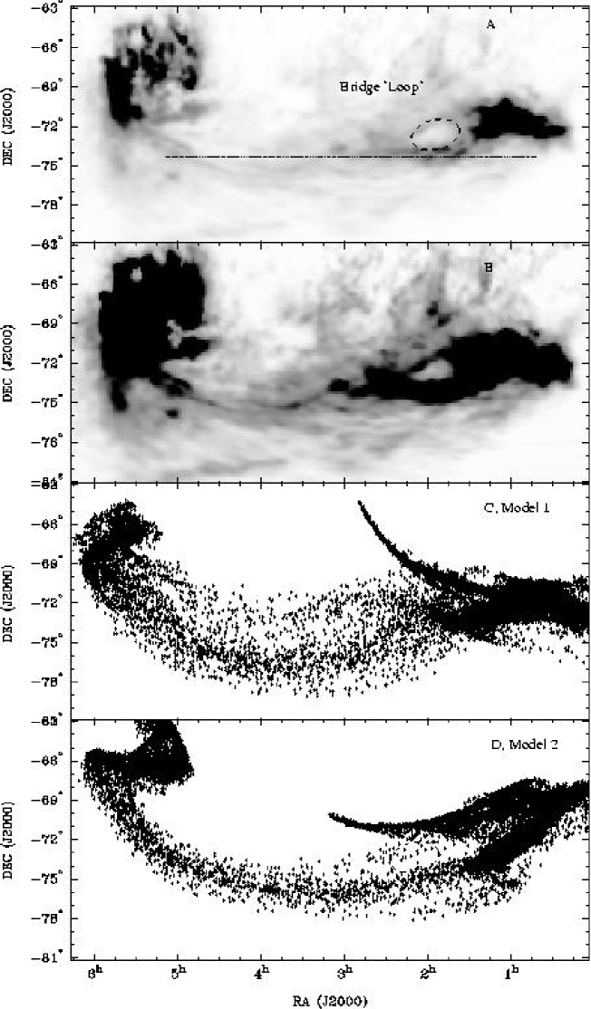
Figure 1: (Top) Panel A (RA,Dec) shows the observed distribution of integrated Hi with the Magellanic Bridge (Brüns et al., 2005). Panel A is strongly contrasted in panel B to highlight the loop feature. the horizontal line indicates $-$73^∘, for reference in Figure2. Panels C and D show the projected distribution of modelled gas-particles for Models 1 and 2 respectively.

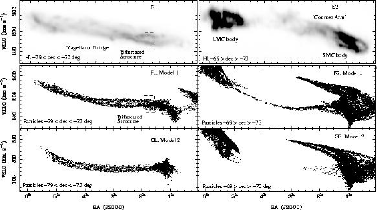
Figure 2: (Top row) Panels E1 and E2 show the RA-velocity projection of neutral hydrogen for $-$79${}^{\circ}<$Dec $<-$73^∘ and $-$69${}^{\circ}>$Dec $>-$73^∘. Panels F1 and F2 show the distribution of simulated gas-particles for Model 1, while panels G1 and G2 show the distribution of gas-particles for Model 2.

From a qualitative study of Figure 1, we see that the large-scale and general filamentary arrangement of the numerical simulations are consistent with observations: the dense ’Bridge’ filament is well reproduced, as well as the central body of the SMC.

The velocity projections in Figure 2 show that the bimodal properties of the densest part of the Bridge can easily be duplicated by Model 1. The two distinct velocity ranges represent similar orbital ’families’ which are present in the Bridge itself. The simulations are able to duplicate the observed velocity separation of $\sim$40km s^-1  as well as the approximate spatial extent of the bimodal arrangement for ${\rm 2^{h}0^{m}}\leq\alpha\leq{\rm 3^{h}0^{m}}$ and 150 km s^-1 $\leq V_{\rm h}\leq$ 200 km s^-1. A significant quantity of material is drawn into the more northerly declinations and out into a velocity range which is different to that of the ’Bridge’ itself.

Both models 1&2 reproduce the SMC as having two filaments: a lower-declination, low-velocity and nearer arm (forming the Bridge proper), and a higher-declination, high-velocity counter-arm component that has more radial extension (See also Figure 4). These results are completely consistent with earlier numerical simulations by Gardiner, Sawa & Fujimoto (1994), and with a quantitative analysis of the turbulent structure of the Hi around the SMC by Muller et al. (2004).

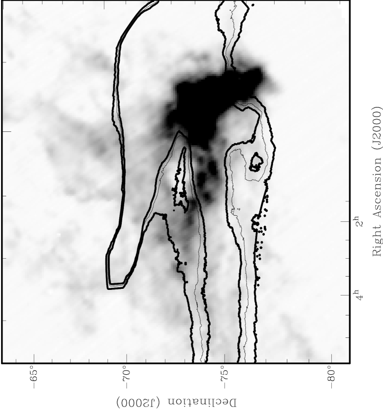
Figure 3: Greyscale: Magnified subregion of the Hi brightness distribution around the SMC (Brüns et al., 2005). Contours: smoothed contours from particles predicted by Model 2. The ’loop’ is central to the figure, and its formation has been clearly reproduced in this simulation. Note that the contour levels are set very low ($<$1%), and so the simulated SMC appears to have a large extent.

Finally, we see in Figure 3 that model 2 can convincingly reproduce the observed ’loop’ off the north-eastern corner of the SMC. Muller et al (2003) report that the loop is found within a contiguous velocity range. A study of their Figures 3 and 4 reveals that the bulk of the loop is consistent with the velocity-shifted northern component, and that the bottom of the loop is delimited by the lower-velocity and brighter southern component.

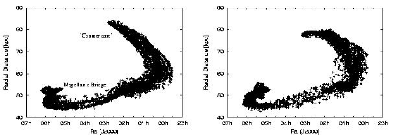
Figure 4: RA and radial position of gas-particles from Models 1 (left) and 2 (right). Both models show the existence of a radially-extending arm. Every 16th point is plotted to reduce crowding.

We show in Figure 4 the position-radius projection of the simulations. We see that in both cases, two filaments emanate from the forming SMC. The actual Magellanic Bridge may be regarded as the more nearby component, whereas the tidal counterpart to the Bridge extends more radially. Importantly, both models predict an extremely large line-of-sight depth for the SMC (including the Bridge, SMC and counter-arm) consistent with some previous numerical simulation results (e.g. Gardiner, Sawa & Fujimoto, 1994); and also a line of sight depth through the Bridge which is consistent with the $\sim$5 kpc line-of-sight measured between adjacent stellar clusters by Demers & Batinelli (1998) in the Magellanic Bridge.

Although neither of the two models can reproduce the observations fully self-consistently, we find that the three key large-scale features in the Magellanic Bridge are produced by these two models. This suggests that the scenario where the Bridge is the result of a tidal interaction between the Clouds and the Galaxy for the last 0.2 Gyr is essentially important in explaining fundamental properties of large-scale organisation of the ISM in the MB.

The lack of exact reproduction at this stage may be due to insufficiently complex simulations, which exclude ISM feedback processes. We note that other large-scale numerical simulations, such as those by Gardiner, Sawa & Fujimoto (1994) are also unable to clearly reproduce the loop feature. Future and more sophisticated models with gas dynamics and star formation will confirm whether the tidal interaction model can explain both the two kinematical properties (i.e., the bimodal kinematics and the velocity offset) and the presence of the giant Hi loop in a self-consistent manner.

4 Alternative loop formation scenarios

Given the preliminary nature of these results in predicting the formation of the Bridge ’loop’, it is appropriate to explore alternative processes which also may develop similar structures such as Hi ’shells’. Processes such as the stellar-wind, SNe and HVC impacts are commonly-cited in the literature as shell-formation mechanisms.

Using the canonical formulations to estimate the total input energy by Weaver et al. (1977) (shell evolution powered by stellar winds) along with data of the basic characteristics of the observed loop (R=1.3 kpc), and based on its observed velocity position in the ’high velocity’ component which has a limiting velocity dispersion of $\sim$30 km s^-1, we estimate an energy requirements for the shell expansion: E_Weav= 53.5 log ergs. Energies of this magnitude are equivalent to that provided by stellar winds, or SNe produced from $\sim$100 O-type stars (Chevalier, 1974). In any other larger system, an association of a few hundred stars would be unremarkable. However, OB associations numbering more than $\sim$10 are uncommon in the Magellanic Bridge (Bica & Schmitt, 1995, ;Bica, priv. comm. 2001) and is not clear how such a relatively well populated association may come to be at the observed location. For this reason, formation of the loop by stellar winds (or SNe) is considered implausible.

Works by Tenorio-Tagle & Bodenheimer (1988) and Tenorio-Tagle et al (1986) have shown through a variety of two dimensional numerical simulations, how an Hi cloud infalling into a stratified gas layer can generate an expanding shell-like structure. From Tenorio-Tagle et al (1986), we can relate the expansion energy of the hole to the kinetic energy of a hypothetical infalling cloud, via the cloud’s density and radius:

n[cm^-3]=9.78$\times$ 10${}^{-43}\frac{E_{kin}}{R_{c}^{3}V_{c}^{2}}$

Using the kinetic energy estimated previously, $E_{kin}$ (erg), we can probe the ranges of HVC properties that are capable of generating a hole having the same observed parameters of the Bridge loop. We find that after limiting the density of the candidate infalling HVC to 0.2$<\rho>$5 cm ^-3, according to the range of HVC densities estimated by Brüns (2003), a 0.6 $\times$10⁶ ${\rm M}_{\odot}$ cloud need only move at a velocity of $\sim$-350 km s^-1 in the LSR frame to attain the estimated kinetic energy to create the observed loop. Such a velocity is not unusual for many of the known HVC population (e.g. Wakker, Osterloo & Putman, 2002; Putman et al., 2002). Recently Bekki & Chiba (2006) have found that massive sub-halos can create kpc-scale giant HI holes such as those seen in the Western Magellanic Bridge. These results imply that if the MB interacted with low-mass subhalos, which are predicted by a hierarchical clustering scenario to be ubiquitous in the Galactic halo region, giant HI holes can be formed. We plan to investigate this possibility in our forthcoming papers.

References

- Abrahamyan (2004) Abrahamyan, H. V, 2004,Ap,47,18
- Berentzen et al. (2001) Berentzen, I., Heller, C. H., Fricke, K. J., Athanassoula, E., 2001, Ap&SS, 276, 699
- de Blok & Walter (2000) de Blok, W. J. G., Walter, F., 2000, ASPC, 218, 357
- Bica & Schmitt (1995) Bica, Eduardo L. D., Schmitt, Henrique R., 1995,ApJS,101,41
- Bloom et al. (2003) Bloom, J. S., Frail, D. A., Kulkarni, S. R., 2003, ApJ, 594, 674
- Brüns et al. (2005) Brüns, C., J.Kerp, L. Staveley-Smith, U.Meabold, M.E., Putman, R.F., Haynes, P.M.W., Kalberla, E. Muller, M.D. Filipovic 2002, 2005, A&A,432,45
- Brüns (2003) Brüns, C , 2003, PhD Thesis, University of Bonn
- Bekki & Chiba (2005) Bekki, K., Chiba, M.,2005,MNRAS,356,680
- Bekki & Chiba (2006) Bekki, K., Chiba, M.,2006,ApJ,637,97
- Broeils & van Woerden (1994) Broeils, A. H., van Woerden, H.,1994,A&AS,107,129
- Chevalier (1974) Chevalier, Roger A., 1974, ApJ, 188, 501
- Connors, Kawata & Gibson (2006) Connors, T., W., Kawata, D., Gibson, B., K.,2006,MNRAS,371,108
- Demers & Batinelli (1998) Demers, S., Battinelli, P., 1998,AJ,115,15
- Gardiner, Sawa & Fujimoto (1994) Gardiner, L. T., Sawa, T., Fujimoto, M., 1994, MNRAS, 266, 567
- Gardiner & Noguchi (1996) Gardiner, L. T., Noguchi, M.,1996,MNRAS,278,191
- Goldman (2000) Goldman, Itzhak, 2000, ApJ, 541, 701
- Lozinskaya, T.A. (1992) Lozinskaya, T.A., in Stellar Wind in the Intersellar Medium, 1992, American Institute of Physics, New York.
- Muller et al (2003) Muller, E., Staveley-Smith, L., Zealey, W., Stanimirović, S., 2003, MNRAS, 339, 105
- Muller et al. (2004) Muller, E., Stanimirović, S., Rosolowsky, E., Staveley-Smith, L., 2004, ApJ, 616, 845
- Navarro, Frenk & White. (1996) Navarro, Julio F., Frenk, Carlos S., White, Simon D. M.,1996,ApJ,462,563
- Putman et al. (2002) Putman, M. E.; de Heij, V.; Staveley-Smith, L.; Braun, R.; Freeman, K. C.; Gibson, B. K.; Burton, W. B.; Barnes, D. G.; Banks, G. D.; Bhathal, R.; and 22 coauthors,2002,AJ,123,873
- Stanimirović, Staveley-Smith & Jones (2004) Stanimirović, S., Staveley-Smith, L., Jones, P. A., 2004,ApJ,604,176
- Staveley-Smith et al. (1997) Staveley-Smith, L., Sault, R. J., Hatzidimitriou, D., Kesteven, M. J., McConnell, D., 1997, MNRAS, 289, 225
- Tenorio-Tagle et al (1986) Tenorio-Tagle, G., Bodenheimer, P., Rozyczka, M., Franco, J., 1986, A&A, 170, 107
- Tenorio-Tagle & Bodenheimer (1988) Tenorio-Tagle, G., Bodenheimer, P.,1988,ARAA,26,145
- Wakker, Osterloo & Putman (2002) Wakker, B. P., Oosterloo, T. A., Putman, M. E., 2002, AJ, 123, 1953
- Wayte (1990) Wayte, S. R.,1990,PhD Thesis, Australian National University
- Weaver et al. (1977) Weaver, R., McCray, R., Castor, J., Shapiro, P., Moore, R., 1977, ApJ, 218, 377
- van der Marel (2002) van der Marel,Roeland P., Alves, David R., Hardy, Eduardo, Suntzeff, Nicholas B.,2002,AJ,124,2639
- Yoshizawa & Noguchi (2004) Yoshizawa, A.M., Noguchi, M., 2004, MNRAS, 339, 1135