Odd-frequency Pairs and Josephson Current through a Strong Ferromagnet

Abstract

We study Josephson current in superconductor / diffusive ferromagnet /superconductor junctions by using the recursive Green function method. When the exchange potential in a ferromagnet is sufficiently large as compared to the pair potential in a superconductor, an ensemble average of Josephson current is much smaller than its mesoscopic fluctuations. The Josephson current vanishes when the exchange potential is extremely large so that a ferromagnet is half-metallic. Spin-flip scattering at junction interfaces drastically changes the characteristic behavior of Josephson current. In addition to spin-singlet Cooper pairs, equal-spin triplet pairs penetrate into a half metal. Such equal-spin pairs have an unusual symmetry property called odd-frequency symmetry and carry the Josephson current through a half metal. The penetration of odd-frequency pairs into a half metal enhances the low energy quasiparticle density of states, which could be detected experimentally by scanning tunneling spectroscopy. We will also show that odd-frequency pairs in a half metal cause a nonmonotonic temperature dependence of the critical Josephson current.

I introduction

Ferromagnetism and spin-singlet superconductivity are competing orders because the exchange potential breaks down spin-singlet pairs. Spin-singlet pairs, however, do not always disappear under the influence of an exchange potential. Long time ago Fulde-Ferrell fulde and Larkin-Ovchinnikov larkin discussed inhomogeneous spin-singlet superconductivity in the presence of an exchange potential. It was shown that the superconducting order parameter oscillates in real space because the exchange potential shifts the center-of-mass momentum of a Cooper pair. Similarly, a Cooper pair has been discussed in superconductor / ferromagnet (SF) and superconductor / ferromagnet / superconductor (SFS) junctions buzdin ; buzdin2 ; petrashov ; ryazanov ; kontos ; golubov ; bergeret ; kadigrobov . These studies showed that a pairing function in a ferromagnet changes its sign periodically in real space. As a consequence, SFS junctions may undergo so-called 0-$\pi$ transition with varying length of a ferromagnet or temperature.

Previous theoretical studies of the proximity effect in a ferromagnet were mainly based on solving the quasiclassical Usadel equations usadel valid when the exchange potential $V_{ex}$ is comparable to or smaller than the pair potential in a superconductor at zero temperature $\Delta_{0}$. Cooper pairs can penetrate into a ferromagnet within a short distance $\xi_{h}=\sqrt{D/V_{ex}}$, where $D$ is the diffusion constant in a ferromagnet. Thus, penetration of spin-singlet Cooper pairs into a ferromagnet with large $V_{ex}$ would be impossible and the Josephson coupling via such a strong ferromagnet would be vanishingly small. A recent experiment robinson , however, demonstrated the existence of Josephson coupling through a strong ferromagnet with $V_{ex}\gg\Delta_{0}$. In addition to this, the experiment keizer has even shown Josephson coupling in superconductor /half metal / superconductor (S/HM/S) junctions. A half metal is an extreme case of a completely spin polarized material because its electronic structure is insulating for one spin direction and metallic for the other. Thus one has to seek a new state of Cooper pairs in a strong ferromagnet. The experiment by Keizer et. al. has motivated a number of theoretical studies in this direction ya07l ; braude ; eschrig2 ; takahasi .

Prior to the experiment keizer , Eschrig et.al. eschrig have addressed this challenging issue. In the clean limit, they have shown that $p$-wave spin-triplet pairs induced by spin-flip scattering at a junction interface can carry Josephson current. In practical S/HM/S junctions, however, a half metal is close to the dirty limit in the diffusive transport regime; the elastic mean free path $\ell$ may be smaller or comparable to the coherence length and is much smaller than the size of the half metal $L_{N}$. Thus, the effects of the impurity potential on the Josephson current should be clarified in a SFS junction consisting of a strong ferromagnet. In this paper, we discuss the Josephson effect in SFS junctions for arbitrary magnitude of $V_{ex}$. When $V_{ex}$ is much larger than $\Delta_{0}$, an ensemble average of the Josephson current is much smaller than its mesoscopic fluctuations altshuler ; zyuzin . Fluctuations of the pairing function in a ferromagnet is responsible for the large fluctuations of Josephson current. The Josephson current vanishes in S/HM/S in the absence of spin-flip scattering at junction interfaces. Spin-flip scattering at junction interfaces drastically changes the characteristic behavior of Josephson current and properties of Cooper pairs in a ferromagnet. Spin-flip scattering allows for the penetration of equal-spin-triplet Cooper pairs which have unusual symmetry property called odd-frequency symmetry bergeret . When the contribution of equal-spin-triplet Cooper pairs to the Josephson current is dominant, the self-averaging property of the Josephson current is recovered. In particular in diffusive S/HM/S junctions, all Cooper pairs in a half metal are in the odd-frequency equal-spin-triplet pairing state ya07l . We also discuss local density of states in a ferromagnet which reflects the existence of odd-frequency Cooper pairs. A part of this study has been already published elsewhere ya07l . Throughout this paper, we use the unit of $\hbar=k_{B}=1$, where $k_{B}$ is the Boltzmann constant.

This paper is organized as follows. In Sec. II, we explain the model of SFS junctions on two-dimensional tight-binding lattice and the method of calculation. The characteristic features of Josephson current in SFS junctions are discussed in Sec. III. In Sec. IV, we introduce spin-flip scattering at junction interfaces and discuss symmetry properties of Cooper pairs in a ferromagnet. We propose an experiment to observe odd-frequency pairs in SFS junctions based on calculated results of local density of states in Sec. V. The conclusions are formulated in Sec. VI.

II model

Let us consider the two-dimensional tight-binding model as shown in Fig. 1(a). A vector $\boldsymbol{r}=j{\boldsymbol{x}}+m{\boldsymbol{y}}$ indicates a lattice site, where ${\boldsymbol{x}}$ and ${\boldsymbol{y}}$ are unit vectors in the $x$ and $y$ directions, respectively. A junction consists of five segments: a ferromagnet ($3\leq j\leq L_{N}-2$), two thin ferromagnetic layers ( $j=$ 1, 2, $L_{N}-1$, and $L_{N}$), and two superconductors ($-\infty\leq j\leq 0$ and $L_{N}+1\leq j\leq\infty$). In the $y$ direction, the number of lattice sites is $W$ and we assume a periodic boundary condition. Electronic states in a superconducting junction are described by the mean-field Hamiltonian

$$H_{\textrm{BCS}}= \frac{1}{2}\sum_{\boldsymbol{r},\boldsymbol{r}^{\prime}}\left[\tilde{c}_{\boldsymbol{r}}^{\dagger}\;{h}_{\boldsymbol{r},\boldsymbol{r}^{\prime}}\;\tilde{c}_{\boldsymbol{r}^{\prime}}-\tilde{c}_{\boldsymbol{r}}^{t}\;{h}^{\ast}_{\boldsymbol{r},\boldsymbol{r}^{\prime}}\;\left\{\tilde{c}_{\boldsymbol{r}^{\prime}}^{\dagger}\right\}^{t}\right]$$

$$+ \frac{1}{2}\sum_{\boldsymbol{r},\boldsymbol{r}^{\prime}\in\textrm{S}}\left[\tilde{c}_{\boldsymbol{r}}^{\dagger}\hat{\Delta}_{\boldsymbol{r},\boldsymbol{r}^{\prime}}\left\{\tilde{c}_{\boldsymbol{r}^{\prime}}^{\dagger}\right\}^{t}-\left\{\tilde{c}_{\boldsymbol{r}}\right\}^{t}\hat{\Delta}^{\ast}_{\boldsymbol{r},\boldsymbol{r}^{\prime}}\tilde{c}_{\boldsymbol{r}^{\prime}}\right],$$ (1)

$$\hat{h}_{\boldsymbol{r},\boldsymbol{r}^{\prime}}= \left[-t\delta_{|\boldsymbol{r}-\boldsymbol{r}^{\prime}|,1}+(\epsilon_{\boldsymbol{r}}-\mu+4t)\delta_{\boldsymbol{r},\boldsymbol{r}^{\prime}}\right]\hat{\sigma}_{0}$$

$$-\boldsymbol{V}(\boldsymbol{r})\cdot\hat{\boldsymbol{\sigma}}\delta_{\boldsymbol{r},\boldsymbol{r}^{\prime}},$$ (2)

$$\hat{\Delta}_{\boldsymbol{r},\boldsymbol{r}^{\prime}}= e^{i\varphi_{j}}i\Delta\hat{\sigma}_{2}\;\delta_{\boldsymbol{r},\boldsymbol{r}^{\prime}},$$ (3)

$$\tilde{c}_{\boldsymbol{r}}= \left(\begin{array}[]{c}c_{\boldsymbol{r},\uparrow}\\ c_{\boldsymbol{r},\downarrow}\end{array}\right),\;\left\{\tilde{c}_{\boldsymbol{r}}\right\}^{t}=(c_{\boldsymbol{r},\uparrow},c_{\boldsymbol{r},\downarrow}),$$ (6)

where $c_{\boldsymbol{r},\sigma}^{\dagger}$ ($c_{\boldsymbol{r},\sigma}$) is the creation (annihilation) operator of an electron at $\boldsymbol{r}$ with spin $\sigma=$ ( $\uparrow$ or $\downarrow$ ), S in the summation means superconductors, $\hat{\sigma}_{j}$ with $j=$1 - 3 are the Pauli matrices, and $\hat{\sigma}_{0}$ is the $2\times 2$ unit matrix. The hopping integral $t$ is considered among the nearest neighbor sites.

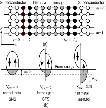
Figure 1: (Color online) (a) A schematic figure of a SFS junction on tight-binding lattice. (b) Density of states for each spin direction. The Josephson junction is of the SNS, SFS, and S/HM/S type for $V_{ex}/t=0$, 1 and 2.5, respectively.

In a ferromagnet, on-site potential is given randomly in a range of $-V_{I}/2\leq\epsilon_{\boldsymbol{r}}\leq V_{I}/2$, where we take the probability distribution for $\epsilon_{\boldsymbol{r}}$ unifom on this interval, and $\epsilon_{\boldsymbol{r}}$ at different points are uncorrelated. The uniform exchange potential in a ferromagnet is given by $\boldsymbol{V}(\boldsymbol{r})=V_{ex}\boldsymbol{e}_{3}$, where $\boldsymbol{e}_{l}$ for $l=1-3$ is a unit vector in spin space. The Fermi energy $\mu$ is set to be $2t$ in a normal metal with $V_{ex}=0$, while a ferromagnet and a half metal are respectively described by $V_{ex}/t$ = 1 and 2.5 as shown in Fig. 1(b). Spin-flip scattering is introduced at $j=1,2$, $L_{N}-1$, and $L_{N}$, where we choose $\boldsymbol{V}(\boldsymbol{r})=V_{S}\boldsymbol{e}_{2}$. In a superconductor, we take $\epsilon_{\boldsymbol{r}}=0$ and $\Delta$ is an amplitude of the pair potential in $s$-wave symmetry. The macroscopic phases are given by $\varphi_{j}=\varphi_{L}$ in the left superconductor and by $\varphi_{j}=\varphi_{R}$ in the right one.

The Hamiltonian is diagonalized by the Bogoliubov transformation,

$$\left[\begin{array}[]{c}\tilde{c}_{\boldsymbol{r}}\\ \left\{\tilde{c}^{\dagger}_{\boldsymbol{r}}\right\}^{t}\end{array}\right]= \sum_{\lambda}\left[\begin{array}[]{cc}\hat{u}_{\lambda}(\boldsymbol{r})&\hat{v}_{\lambda}^{\ast}(\boldsymbol{r})\\ \hat{v}_{\lambda}(\boldsymbol{r})&\hat{u}_{\lambda}^{\ast}(\boldsymbol{r})\end{array}\right]\left[\begin{array}[]{c}\tilde{\gamma}_{\lambda}\\ \left\{\tilde{\gamma}^{\dagger}_{\lambda}\right\}^{t}\end{array}\right],$$ (13)

$$\tilde{\gamma}_{\lambda}= \left(\begin{array}[]{c}\gamma_{\lambda,\uparrow}\\ \gamma_{\lambda,\downarrow}\end{array}\right),$$ (16)

where ${\gamma}^{\dagger}_{\lambda,\sigma}$ (${\gamma}_{\lambda,\sigma}$) is the creation (annihilation) operator of a Bogoliubov quasiparticle. The wave functions, $\hat{u}_{\lambda}$ and $\hat{v}_{\lambda}$, satisfy the Bogoliubov-de Gennes equation degennes ,

$$\sum_{\boldsymbol{r}^{\prime}} \left[\begin{array}[]{cc}\hat{h}_{\boldsymbol{r},\boldsymbol{r}^{\prime}}&\hat{\Delta}_{\boldsymbol{r},\boldsymbol{r}^{\prime}}\\ -\hat{\Delta}^{\ast}_{\boldsymbol{r},\boldsymbol{r}^{\prime}}&-\hat{h}^{\ast}_{\boldsymbol{r},\boldsymbol{r}^{\prime}}\end{array}\right]\left[\begin{array}[]{c}\hat{u}_{\lambda}(\boldsymbol{r}^{\prime})\\ \hat{v}_{\lambda}(\boldsymbol{r}^{\prime})\end{array}\right]=\left[\begin{array}[]{c}\hat{u}_{\lambda}(\boldsymbol{r})\\ \hat{v}_{\lambda}(\boldsymbol{r})\end{array}\right]\hat{E}_{\lambda}.$$ (23)

The eigen value matrix $\hat{E}_{\lambda}$ is diagonal and depends on spin channels. To solve the Bogoliubov-de Gennes equation, we apply the recursive Green function method furusaki ; ya01-1 . In this method, we calculate the Matsubara Green function

$$\check{G}_{\omega_{n}}(\boldsymbol{r},\boldsymbol{r}^{\prime}) =\sum_{\lambda}\left[\begin{array}[]{c}\hat{u}_{\lambda}(\boldsymbol{r})\\ \hat{v}_{\lambda}(\boldsymbol{r})\end{array}\right][i\omega_{n}-\hat{E}_{\lambda}]^{-1}\left[\hat{u}_{\lambda}^{\dagger}(\boldsymbol{r}^{\prime}),\hat{v}_{\lambda}^{\dagger}(\boldsymbol{r}^{\prime})\right]$$ (26)

$$+ \left[\begin{array}[]{c}\hat{v}^{\ast}_{\lambda}(\boldsymbol{r})\\ \hat{u}^{\ast}_{\lambda}(\boldsymbol{r})\end{array}\right][i\omega_{n}+\hat{E}_{\lambda}]^{-1}\left[\hat{v}_{\lambda}^{t}(\boldsymbol{r}^{\prime}),\hat{u}_{\lambda}^{t}(\boldsymbol{r}^{\prime})\right],$$ (29)

$$=\left(\begin{array}[]{cc}\hat{g}_{\omega_{n}}(\boldsymbol{r},\boldsymbol{r}^{\prime})&\hat{f}_{\omega_{n}}(\boldsymbol{r},\boldsymbol{r}^{\prime})\\ -\hat{f}_{\omega_{n}}^{\ast}(\boldsymbol{r},\boldsymbol{r}^{\prime})&-\hat{g}_{\omega_{n}}^{\ast}(\boldsymbol{r},\boldsymbol{r}^{\prime})\end{array}\right),$$ (32)

where $\omega_{n}=(2n+1)\pi T$ is a Matsubara frequency, $n$ is an integer number, and $T$ is the temperature. The Josephson current is given by

$$J=-ietT\sum_{\omega_{n}}\sum_{m=1}^{W}\mathrm{Tr}\left[\check{G}_{\omega_{n}}(\boldsymbol{r}^{\prime},\boldsymbol{r})-\check{G}_{\omega_{n}}(\boldsymbol{r},\boldsymbol{r}^{\prime})\right]$$ (33)

with $\boldsymbol{r}^{\prime}=\boldsymbol{r}+\boldsymbol{x}$. In this paper, $2\times 2$ and $4\times 4$ matrices are indicated by $\hat{\cdots}$ and $\check{\cdots}$, respectively.

In simulations, we first compute the Josephson current for a single sample with a specific random impurity configuration. After calculating the Josephson current over a number of different samples, an ensemble average of the Josephson current and its fluctuations are obtained as

$$\langle J\rangle= \frac{1}{N_{s}}\sum_{i=1}^{N_{s}}J_{i},$$ (34)

$$\delta J= \sqrt{\langle J^{2}\rangle-\langle J\rangle^{2}},$$ (35)

where $J_{i}$ is the Josephson current in the $i$ th sample and $N_{s}$ is the number of samples. Strictly speaking, $N_{s}$ should be taken to be infinity. In this paper, we increase $N_{s}$ until sufficient convergence of $\langle J\rangle$ and $\delta J$ is obtained. In the following, $N_{s}$ is typically taken to be 100-2000.

To study the characteristics of Cooper pairs in a ferromagnet, we also analyze the anomalous Green function in Eq. (32). The pairing function is defined by the anomalous Green function and is decomposed into four components,

$$\sum_{\omega_{c}<\omega_{n}<\Delta_{0}}\frac{1}{W}\sum_{m=1}^{W}\hat{f}_{\omega_{n}}(\boldsymbol{r},\boldsymbol{r})=i\sum_{\nu=0}^{3}f_{\nu}(j)\hat{\sigma}_{\nu}\hat{\sigma}_{2},$$ (36)

where $\boldsymbol{r}=j\boldsymbol{x}+m\boldsymbol{y}$, $\omega_{c}=0.01\Delta_{0}$ is a low energy cut-off and the pairing functions are averaged over whole lattice sites at $j$ before ensemble averaging. In Eq. (36), $f_{0}(f_{3})$ is the pairing function of spin-singlet (spin-triplet) pairs with spin structure of $(\left|\uparrow\downarrow\right\rangle-(+)\left|\downarrow\uparrow\right\rangle)/\sqrt{2}$. The pairing functions of $\left|\upuparrows\right\rangle$ and $\left|\downdownarrows\right\rangle$ pairs are given by $f_{\uparrow\uparrow}=if_{2}-f_{1}$ and $f_{\downarrow\downarrow}=if_{2}+f_{1}$, respectively.

The quasiclassical Green function method eilenberger ; usadel is a powerful tool to study the proximity effect when the pair potential is much smaller than the Fermi energy. The quasiclassical Green function, however, cannot be constructed in a half metal because the Fermi energy for one spin direction is no longer much larger than the pair potential. On the other hand, there is no such difficulty in our method. These are advantages of the recursive Green function method. Throughout this paper we fix the following parameters: $L_{N}=74$, $W=25$, $\mu=2t$, and $V_{I}=2t$. This parameter choice corresponds to the diffusive transport regime in the N, F and HM layers length . The results presented below are not sensitive to variations of these parameters.

III SFS junction without spin-active interface

In this section, we do not consider spin-flip scattering at the interfaces, (i.e., $V_{S}=0$). We first discuss the Josephson current in SFS junctions as shown in Fig. 2, where $T=0.1T_{c}$, $\Delta_{0}=0.01t$, $T_{c}$ is the superconducting transition temperature, and the phase difference across a junction $\varphi=\varphi_{L}-\varphi_{R}$ is fixed at $\pi/2$.

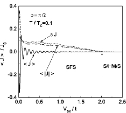
Figure 2: Josephson current is plotted as a function of the exchange potential $V_{ex}$ for $V_{S}=0$ and $\Delta_{0}=0.01t$. At $V_{ex}=2t$, a ferromagnet becomes half-metallic as indicated by an arrow. The vertical axis is normalized by $J_{0}$ which is an ensemble average of Josephson current at $V_{ex}=0$. The number of samples used for averaging $N_{s}$ is 500.

The presented results are normalized by $J_{0}$ which is the ensemble averaged of Josephson current in the superconductor / normal metal / superconductor (SNS) junctions (i.e., $V_{ex}=0$). The Josephson current oscillates as a function of $V_{ex}$ and changes its sign almost periodically. The sign changes of $\langle J\rangle$ correspond to the 0-$\pi$ transition of a SFS junction. At the same time, the amplitude of $\langle J\rangle$ decreases rapidly with increasing $V_{ex}$. For $V_{ex}>0.1t$, we should pay attention to the relation $\langle J\rangle\ll\delta J$ which means that the Josephson current is not a self-averaging quantity. It is impossible to predict the Josephson current in a single sample $J_{i}$ from $\langle J\rangle$ because $J_{i}$ strongly depends on the microscopic impurity configuration. In fact, the Josephson current flows in a single sample even if $\langle J\rangle=0$ at the transition points. Roughly speaking, $\langle J\rangle$ vanishes because half of samples are 0-junctions and the rest are the $\pi$-junctions zyuzin ; ya01-2 . Since $\langle J\rangle=0$, $\delta J$ approximately corresponds to the typical amplitude of the Josephson current expected in a single sample. In Fig. 2, we also show $\langle|J|\rangle$, which agrees well with $\delta J$ even quantitatively. The relation $\langle J\rangle=0$ has different meaning for SFS and S/HM/S cases. In a SFS junction, the fact that $\langle J\rangle=0$ at the transition points is a result of ensemble averaging and the Josephson current remains finite in a single sample. The characteristic temperature and length of a ferromagnet at the $0-\pi$ transitions vary from one sample to another. In S/HM/S junctions at $V_{ex}=2.5t$, however, $\langle J\rangle=0$ means that the Josephson current vanishes even in a single sample because $\delta J=0$ holds at the same time.

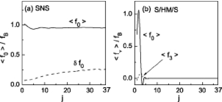
Figure 3: Pairing functions are plotted as a function of position $j$ for (a) SNS at $V_{ex}/t=0$ and (b) S/HM/S at $V_{ex}/t=2.5$, where $V_{S}=0$, $\Delta_{0}=0.01t$ and $N_{s}=200$. The vertical axis is normalized by a pairing function in a superconductor $f_{B}$.

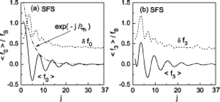
Figure 4: Pairing functions in SFS junctions with $V_{ex}/t=1$, $V_{S}=0$, $\Delta_{0}=0.01t$ and $N_{s}=$500.

The large fluctuations of Josephson current were discussed by Zyuzin et. al. zyuzin by using the diagrammatic expansion. An ensemble average of critical Josephson current and its fluctuations have a relation for $W\gg L_{N}$

$$\frac{\delta J}{\langle J\rangle}\sim \sqrt{\frac{1}{W}}\frac{\exp(-L_{N}/\xi_{T})}{\exp(-L_{N}/\xi_{h})},$$ (37)

$$\sim \sqrt{\frac{1}{W}}\exp\left\{(\sqrt{V_{ex}}-\sqrt{\Delta_{0}})/\sqrt{E_{Th}}\right\},$$ (38)

where $E_{Th}=D/L_{N}^{2}$ is the Thouless energy, $\xi_{T}=\sqrt{D/2\pi T}$, and $\xi_{h}=\sqrt{D/V_{ex}}$ is estimated to be about four lattice constants (See also Appendix A). In the second line, we replace $T$ by $\Delta_{0}$ because a measuring temperature must be smaller than $T_{c}$. For a weak ferromagnet (i.e., $V_{ex}\lesssim\Delta_{0}$), the ratio can be less than unity and the Josephson current is a self-averaging quantity. On the other hand, in a strong ferromagnet with $V_{ex}\gg\Delta_{0}$, the ratio becomes much larger than unity. Thus the large fluctuation of Josephson current is a robust feature of SFS junctions with $V_{ex}\gg\Delta_{0}$. The only way to suppress fluctuations is taking the junction width sufficiently large because fluctuations are a mesoscopic effect.

The origin of the large fluctuations in the Josephson current can be understood by analyzing pairing functions of Cooper pairs. We plot a pairing function of spin-singlet pairs $f_{0}$ in an SNS junction as a function of position in a normal metal $j$ in Fig. 3(a), where $j=1$ and 37 correspond respectively to the junction interface and the center of the normal metal. The pairing function is calculated for $\varphi=0$ and is normalized by its bulk value in a superconductor $f_{B}$. In SNS junctions, $\langle f_{0}\rangle$ is a real value and is almost constant as shown in Fig. 3(a), which means that spin-singlet Cooper pairs exist everywhere in the normal metal. The pairing function for spin-singlet pairs in SFS junctions is shown in Fig. 4(a). An average $\langle f_{0}\rangle$ decreases exponentially with $j$ according to $\exp(-j/\xi_{h})$. At the same time, $\langle f_{0}\rangle$ oscillates in real space and changes its sign. In addition to spin-singlet pairs, opposite-spin-triplet pairs appear in a ferromagnet for $V_{ex}\neq 0$. Since $f_{3}$ is a pure imaginary value, the imaginary part of $\langle f_{3}\rangle$ is plotted in Fig. 4(b). The behavior of $\langle f_{3}\rangle$ is qualitatively the same as that of $\langle f_{0}\rangle$ in Fig. 4(a). Thus opposite-spin-triplet pairs also contribute to the Josephson current. Both $\delta f_{0}$ and $\delta f_{3}$ remain finite at the center of a ferromagnet $j=37$. Spin-singlet and opposite-spin-triplet pairs penetrate deeply into a ferromagnet far beyond $\xi_{h}$ even though $\langle f_{0}\rangle$ and $\langle f_{3}\rangle$ are almost zero there. We numerically confirm the relation $\delta f_{0}\propto e^{-j/\xi_{T}}$, in agreement with Ref. zyuzin, .

In Fig. 5 (a) and (b), we show $f_{0}$ and $f_{3}$ in SFS junctions for three samples with different impurity distribution. The vertical axis is shifted as indicated by horizontal lines. The pairing functions are in phase near the interface ($j\leq\xi_{h}$), whereas they are out of phase far from the interface. Although the pairing function in a sample has a finite value for $j>\xi_{h}$, an ensemble average of them vanishes. Cooper pairs do exist in a single sample of ferromagnet even for $j\gg\xi_{h}$. Mesoscopic fluctuations of the pairing function provide the origin of the large fluctuations in the Josephson current. In S/HM/S junctions, as shown in Fig. 3(b), $\langle f_{0}\rangle$ and $\langle f_{3}\rangle$ vanish for $j\gg 1$. We have also confirmed that $\delta f_{0}=\delta f_{3}=0$ for $j\gg 1$ at the same time. Thus, no Cooper pairs exist in a half metal for $V_{S}=0$.

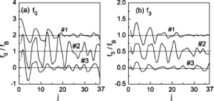
Figure 5: Pairing functions in three different samples of SFS junction at $V_{ex}/t=1$.

Since $\langle J\rangle\ll\delta J$, the temperature dependence of Josephson current also depends on the impurity configuration. In Fig. 6, we show the Josephson critical current as a function of temperature for five different samples, where the critical current is estimated from the current-phase relation at each temperature. The solid line in Fig. 6(a) corresponds to a SFS junction in the 0-state, where the critical current monotonically increases with the decrease of temperature. On the other hand, the broken line corresponds to a junction in the $\pi$-state. In Fig. 6(b), a junction undergoes the transition from 0 to $\pi$ state when temperature decreases across 0.5$T_{c}$. On the contrary, the $0-$state is more stable than the $\pi-$state at low temperatures in Fig. 6(c). The Josephson current is decomposed into a series of $J=\sum_{k=1}J_{k}\sin(k\varphi)$. In Fig. 6, $J_{1}=0$ characterizes the 0-$\pi$ transition temperature. At the transition temperature, the critical current is not exactly zero because a higher harmonic such as $J_{2}\sin(2\varphi)$ contributes to the Josephson current. Some SFS junctions undergo the 0-$\pi$ transition twice as shown in Fig. 6(d). The temperature dependence of the critical current in one sample can be very different from that in another samples.

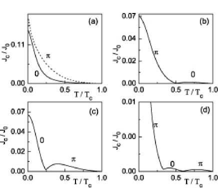
Figure 6: Critical current versus temperatures for five different samples of SFS junction, where $V_{ex}/t=1$, $V_{S}=0$, and $\Delta_{0}/t=0.01$.

IV SFS junction with spin-active interface

The relation $\langle J\rangle\ll\delta J$ is a characteristic feature of the Josephson current in diffusive SFS junctions with $V_{ex}\gg\Delta_{0}$. This feature, however, is drastically changed by spin-flip scattering at junction interfaces. In this section, we study the Josephson current in the presence of spin-flip scattering, (i.e., $V_{S}\neq 0$).

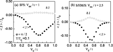
Figure 7: (a) Josephson current and its fluctuations for $T=0.1T_{c}$, $\varphi=\pi/2$ and $N_{s}=200$ as a function of interface spin-flip scattering $V_{S}$ for $V_{ex}/t=1$ and (b) for $V_{ex}/t=2.5$. The vertical axis is normalized by an ensemble average of Josephson current at $V_{ex}=0$ and $V_{S}=0$.

In Figs. 7 (a) and (b), we show $\langle J\rangle$ as a function of the spin-flip potential $V_{S}$ for $V_{ex}/t=1$ and 2.5, respectively. In both cases (a) and (b), we find that $|\langle J\rangle|\geq\delta J$ for $V_{S}\geq 0.3t$. The Josephson current recovers the self-averaging property in the presence of spin-flip scattering. Reasons can be found by analyzing the pairing functions in a ferromagnet, as shown in Figs. 8 and 9, where four pairing functions are plotted as a function of position $j$ at $V_{S}/t=0.4$. In SFS junctions as shown in Fig. 8(a), equal-spin-triplet Cooper pairs penetrate into a ferromagnet by spin-flip scattering at interfaces. Although averages of the pairing function for opposite-spin pairs vanish at $j\sim 37$, their fluctuations remain finite as shown in Figs. 8(a) and (b). Thus four types of Cooper pairs carry the Josephson current in a SFS junction. In a S/HM/S junction, on the other hand, only $\uparrow\uparrow$-pairs exist in a half metal as shown in Fig. 9(a) and (b). The pairing functions $\langle f_{\downarrow\downarrow}\rangle$, $\langle f_{0}\rangle$, and $\langle f_{3}\rangle$ vanish for $j\gg 1$. We note that fluctuations of these pairing functions behave similar to their averages. In both SFS and S/HM/S, $\langle f_{\uparrow\uparrow}\rangle$ becomes much larger than $\delta f_{0}$ because the exchange potential does not break down equal-spin-triplet Cooper pairs and $f_{\uparrow\uparrow}$ does not suffer sign change in real space. Thus the Josephson current becomes a self-averaging quantity as shown in Figs. 7(a) and (b).

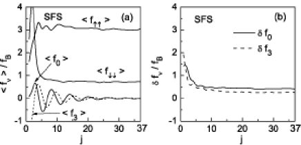
Figure 8: Pairing functions in SFS junctions are plotted as a junction of $j$. Ensemble averages and some of their fluctuations are shown in (a) and (b), respectively. The number of samples are taken to be 500.

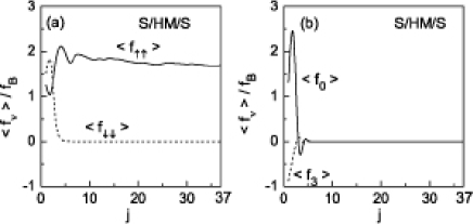
Figure 9: Pairing functions in S/HM/S junctions are plotted as a junction of $j$. The number of samples are taken to be 200.

Here we address an unusual symmetry property of Cooper pairs in SFS junctions. In Fig. 10, we show four pairing functions in a SFS junction as a function of $\omega_{n}$, where $j=37$, $V_{S}=0.2t$, $\varphi=0$, and $V_{ex}=t$. Although the Green function at $\omega_{n}=0$ is not defined, we put $f_{\uparrow\uparrow}=f_{\downarrow\downarrow}=f_{3}=0$ at $\omega_{n}=0$, and connect results for positive $\omega_{n}$ with those for negative $\omega_{n}$. The pairing function $f_{0}$ is an even function of $\omega_{n}$, whereas $f_{\uparrow\uparrow}$, $f_{\downarrow\downarrow}$, and $f_{3}$ are an odd function of $\omega_{n}$ bergeret . Since electrons obey Fermi statistics, pairing functions must be antisymmetric under interchanging two electrons,

$$\hat{f}_{\omega_{n}}(\boldsymbol{r},\boldsymbol{r}^{\prime})=-\left[{\hat{f}}_{-\omega_{n}}(\boldsymbol{r}^{\prime},\boldsymbol{r})\right]^{t},$$ (39)

where $[\hat{f}]^{t}$ denotes the transpose of $\hat{f}$ meaning the interchange of spins. It is well known that ordinary even-frequency pairs are classified into two symmetry classes: spin-singlet even-parity symmetry and spin-triplet odd-parity one. In the former case, the negative sign on the right hand side of Eq. (39) arises due to the interchange of spins, while in the latter case due to $\boldsymbol{r}\leftrightarrow\boldsymbol{r}^{\prime}$. In the present calculation, all components on the right hand side of Eq. (36) have $s$-wave symmetry. This is because the pairing functions are isotropic in both real and momentum spaces due to diffusive impurity scatterings tanaka06 . As a result, $f_{\uparrow\uparrow}$, $f_{\downarrow\downarrow}$, and $f_{3}$ must be an odd function of $\omega_{n}$ to obey Eq. (39). The fraction of odd-frequency pairs depends on parameters such as the exchange potential and the spin-flip potential. As shown Fig. 3(a), all Cooper pairs have even-frequency symmetry in SNS junctions at $V_{ex}=0$ and $V_{S}=0$. Even- and odd-frequency pairs have almost same fraction in SFS junctions at $V_{ex}=t$ and $V_{S}=0$ as shown in Fig. 4. In the presence of spin-flip potential, odd-frequency pairs become dominant as shown in Fig. 8. In particular, all Cooper pairs have odd-frequency symmetry in S/HM/S junctions as shown in Fig. 9. The Josephson current in Fig. 7(b) is carried purely by odd-frequency pairs in S/HM/S junctions.

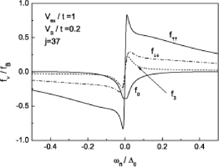
Figure 10: Pairing functions in a SFS junction are plotted as a junction of $\omega_{n}$ for $V_{ex}/t=1$ and $V_{S}/t=0.2$.

The results in Fig. 7 show that the amplitude of Josephson current first increases with the increase of $V_{S}$ then decreases. Here we discuss the analytical expression of the Josephson current in S/HM/S junction at $T=0$,

$$\langle J\rangle=-J_{1}$$

$$\times\left[\left(\boldsymbol{V}_{L}\cdot\boldsymbol{V}_{R}-{V}_{L}^{(3)}{V}_{R}^{(3)}\right)\sin\varphi+\boldsymbol{e}_{3}\cdot(\boldsymbol{V}_{L}\times\boldsymbol{V}_{R})\cos\varphi\right],$$ (40)

$$J_{1}=\frac{7\zeta(3)}{\pi}eE_{Th}\;g_{N}b^{2}>0,$$ (41)

$$b=\frac{1}{2}\int_{0}^{\pi/2}\!\!\!\!d\gamma\;\frac{\cos^{5}\gamma}{\left(V_{S}^{2}+\frac{1}{4}\right)\cos^{4}\gamma-V_{S}^{2}\cos^{2}\gamma+V_{S}^{4}}.$$ (42)

Here $\boldsymbol{V}_{R}=\sum_{k=1}^{3}V_{R}^{(k)}\boldsymbol{e}_{k}$ and $\boldsymbol{V}_{L}=\sum_{k=1}^{3}V_{L}^{(k)}\boldsymbol{e}_{k}$ are the dimensionless magnetic moments at the right and left junction interface, respectively. We assume that $|\boldsymbol{V}_{R}|=|\boldsymbol{V}_{L}|=V_{S}$ and $(e^{2}/h)g_{N}$ is the normal conductance of a half metal. Details of derivation are discussed in Appendices A and B. To compare Eq.(40) with the results in Fig. 7(b), we choose $\boldsymbol{V}_{R}=\boldsymbol{V}_{L}=V_{S}\boldsymbol{e}_{2}$. We also note that the magnetic moment in a half metal is $\boldsymbol{V}_{ex}=V_{ex}\boldsymbol{e}_{3}$. For $V_{S}\ll 1$, the amplitude of the Josephson current increases with $V_{S}^{2}$ because $b=2$ and $\boldsymbol{V}_{L}\cdot\boldsymbol{V}_{R}-{V}_{L}^{(3)}{V}_{R}^{(3)}=V_{S}^{2}$. In this case, spin-flip scattering assists the Josephson current. For large $V_{S}$, on the other hand, the Josephson current decreases proportionally to $V_{S}^{-6}$ because the spin-flip potential acts like a potential barrier and suppresses the transmission probability of the interface. The Josephson current shows reentrant behavior as shown in Fig. 7. The Josephson current in Fig. 7(b) is calculated at $\varphi=\pi/2$. The results indicate that the S/HM/S junction is a $\pi$-junction. This conclusion depends on the direction of the magnetic moments at the spin-flip interfaces. In the case of $\boldsymbol{V}_{L}=\boldsymbol{V}_{R}$, the Josephson current in Eq. (40) is proportional to $-J_{1}\sin\varphi$ in agreement with Fig. 7(b). In the case of antiferromagnetic alignment, $\boldsymbol{V}_{L}=-\boldsymbol{V}_{R}$, the junction is in the 0-state. Thus we conclude that the stability of the $0$-state and that of the $\pi$-state depend on the alignment of the magnetic moments at the two interfaces volkov ; houzet1 . This feature indicates a new direction to controlling the $\pi$-phase shift by using ferromagnetic materials. For $\boldsymbol{V}_{ex}\cdot(\boldsymbol{V}_{L}\times\boldsymbol{V}_{R})\neq 0$, the Josephson current flows even at $\varphi=0$ because such spin configuration breaks the chiral symmetry of a junction. We have numerically confirmed the Eq. (40).

In the end of this section, we discuss the temperature dependence of the Josephson critical current in SFS and S/HM/S junctions in Fig. 11, where we choose $\Delta_{0}=0.005t$ in connection with the density of states in the next section.

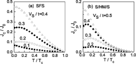
Figure 11: Temperature dependence of critical Josephson current in SFS (a) and S/HM/S (b) junctions. $N_{s}$ is taken to be 200.

The Josephson current has almost a sinusoidal current-phase relationship. The critical current for $V_{S}/t=0.2$ and 0.3 in a SFS junction first increases with the decrease of temperature then decreases as shown in Fig. 11(a). Such reentrant behavior is seen more clearly in a S/HM/S junction as shown for $V_{S}/t=0.2$, 0.3 and 0.4 in Fig. 11(b). In a Josephson junction consisting of conventional $s$-wave spin-singlet superconductors, such reentrant behavior is very unusual. This behavior has also been reported in Ref. eschrig2, . The results for $V_{S}/t=0.4$ in SFS and $V_{S}/t=0.5$ in S/HM/S junctions, on the other hand, show a monotonic temperature dependence.

V density of states

The proximity effect changes the low energy spectra of a quasiparticle in a normal metal. In a SNS junction, it is well known that the penetration of usual even-frequency spin-singlet $s$-wave Cooper pairs suppresses the quasiparticle density of states for $E<E_{Th}$. This suppressed density of states is called minigap. In this section, we discuss the proximity effect of odd-frequency pairs on the quasiparticle density of states. In our method, the density of states is given by

$$N(E,j)=-\frac{1}{\pi}\frac{1}{W}\sum_{m=1}^{W}\text{Im}\text{Tr}\check{G}_{E+i\gamma}(\boldsymbol{r},\boldsymbol{r}),$$ (43)

where $\gamma$ is a small imaginary part. In Fig. 12, we show the local density of states (LDOS) at $j=37$ in SFS junctions, where $\varphi=0$, and $\gamma=0.1\Delta_{0}$. The results for S/HM/S junctions are presented in Fig. 13. The LDOS is normalized by its value at $E=1.2\Delta_{0}$. Here we choose $\Delta_{0}=0.005t$ so that $E_{Th}\sim 0.3\Delta_{0}$ is slightly smaller than $\Delta_{0}$. In the absence of spin-flip scattering, the ensemble average of LDOS is almost constant in both Figs. 12 and  13. At $V_{S}/t=0.3$, the penetration of odd-frequency pairs enhances LDOS for $E<0.5\Delta_{0}$. On the other hand, LDOS is suppressed around $E\sim 0.8\Delta_{0}$ because of a sum rule for the density of states (i.e., $\int dE\;N(E,j)=const.$). The low energy spectra of LDOS increase with increasing $V_{S}/t$ as shown in Figs. 12(b) and 13(b). At $V_{S}/t=0.5$, LDOS has a peak at $E=0$. Thus the penetration of odd-frequency pairs enhances the quasiparticle density of states for $E<E_{Th}$. This tendency is just opposite to the minigap structure due to penetration of even-frequency pairs. The shape of the zero-energy peak in Figs. 12(b) and 13(b) is almost independent of the position in a half metal. The peak is much stronger than the enhancement of the LDOS found in weak ferromagnets buzdin ; golubov ; fogelstrom ; kontos2 ; yokoyama . In such SF junctions kontos2 , the LDOS has an oscillatory peak/dip structure at $E=0$, which rapidly decays with the distance from the SF interface. Therefore, the large peak at $E=0$ in the LDOS is a robust and direct evidence of the odd-frequency pairing in a ferromagnet. Scanning tunneling spectroscopy (STS) could be used to detect such a peculiar pairing state.

As shown in Fig. 13, however, the penetration of odd-frequency pairs does not always give rise to a zero-energy peak in LDOS. The results for $V_{S}/t=0.3$ and 0.4 have a broad peak at a finite energy smaller than $E_{Th}$. This situation is slightly different from the large zero-energy peak in a normal metal due to the penetration of odd-frequency pairs from spin-triplet odd-parity superconductors yt04 ; yt05r ; ya06l ; ya07-2 . In a spin-triplet superconductor junction, LDOS in a normal metal always has a large zero-energy peak because a midgap Andreev resonant state yt95l assists the zero-bias peak. In ferromagnetic junctions, on the other hand, such a quasiparticle state is absent at the junction interface.

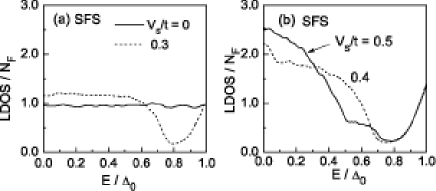
Figure 12: Local density of states at $j=37$ in a ferromagnet of SFS junction, where $N_{s}=2000$.

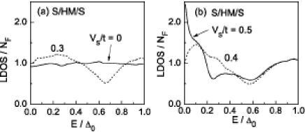
Figure 13: Local density of states at $j=37$ in a half metal of S/HM/S junction, where $N_{s}=2000$.

The broad peak structure in the LDOS is responsible for the nonmonotonic temperature dependence of the critical current in Fig. 11(b). At high temperatures, quasiparticle states around the peak contribute to the Josephson current. At low temperatures, however, such quasiparticle states cannot contribute to the Josephson current ya02-4 . We conclude that odd-frequency pairs could also be confirmed by measuring the dependence of the critical current on temperature.

VI conclusion

In conclusion, we have studied the Josephson effect in superconductor / diffusive ferromagnet / superconductor (SFS) junctions by using the recursive Green function method. When the exchange potential in a ferromagnet is much larger than the pair potential in a superconductor, the Josephson current is not a self-averaging quantity. This is because spin-singlet Cooper pairs penetrating into a ferromagnet far beyond $\xi_{h}$ cause large fluctuations of the pairing function. As a consequence, the temperature dependence of the critical Josephson current in one sample can be very different from that in another sample. When a ferromagnet is half-metallic, the Josephson current vanishes in the absence of spin-flip scattering at junction interfaces. Spin-flip scattering at interfaces allows equal-spin-triplet odd-frequency Cooper pairs to penetrate into a ferromagnet. The ratio of odd-frequency pairs to even-frequency ones depends on the exchange potential in a ferromagnet and the spin-flip potential at interfaces. The Josephson current recovers the self-averaging property when the fraction of equal-spin-triplet pairs becomes large. In half-metallic SFS junctions, all Cooper pairs have odd-frequency symmetry. The penetration of odd-frequency pairs enhances low energy quasiparticle density of states in a ferromagnet. Such low energy spectra could be probed by scanning tunneling spectroscopy and determining a nonmonotonic temperature dependence of the critical Josephson current. We also discuss a way to realize a $\pi$-junction by controlling magnetic moments in ferromagnetic layers.

Appendix A fluctuations of Josephson current

The purpose of this appendix is to explain Eq. (37). Since fluctuations of Josephson current have been calculated by the diagrammatic expansion altshuler ; zyuzin ; koyama , we also calculate the Josephson current in SFS junctions in the same method. We assume that relations $E_{Th}\ll\Delta_{0},V_{ex}\ll\mu$ and $L_{N}\gg\ell$ are satisfied. In the lowest coupling, the Josephson current is given by a formula ya01-3

$$J={ie}\sum_{{l},{r}}T\sum_{\omega_{n}}\textrm{Tr}\left[\hat{r}^{eh}_{l}\cdot\hat{t}^{h}_{lr}\cdot\hat{r}^{he}_{r}\cdot\hat{t}^{e}_{rl}-\hat{r}^{he}_{l}\cdot\hat{t}^{e}_{lr}\cdot\hat{r}^{eh}_{r}\cdot\hat{t}^{h}_{rl}\right],$$ (44)

where $l$ ($r$) denotes a propagating channel at the left (right) junction interface. In Fig. 14(a), a propagation process of the first term in Eq. (44) is schematically illustrated. We calculate the transmission coefficients in a ferromagnet such as $\hat{t}^{e}_{rl}$ and $\hat{t}^{h}_{lr}$ and Andreev reflection coefficients at interfaces such as $\hat{r}^{he}_{r}$ and $\hat{r}^{eh}_{l}$ by parts. The Andreev reflection coefficients are calculated at an ideal NS interface as shown in the left figure of Fig. 14(b). The results are given by

$$\hat{r}^{he}_{l(r)}= -\hat{\sigma}_{2}\frac{\Delta_{0}}{\omega_{n}+\Omega_{n}}\;e^{-i\varphi_{L(R)}},$$ (45)

$$\hat{r}^{eh}_{l(r)}= \hat{\sigma}_{2}\;\frac{\Delta_{0}}{\omega_{n}+\Omega_{n}}e^{i\varphi_{L(R)}},$$ (46)

where $\Omega_{n}=\sqrt{\omega_{n}^{2}+\Delta_{0}^{2}}$. The effect of the exchange potential is considered through transmission coefficients of an electron in a ferromagnet

$$\hat{t}_{lr}^{e}=\left(\begin{array}[]{cc}t^{e}_{lr}(\uparrow)&0\\ 0&t^{e}_{lr}(\downarrow)\end{array}\right).$$ (49)

The transmission coefficients of a hole are defined in the same way by $e\to h$ in the equation above. The transmission coefficients are represented by the Green function as

$$t^{e}_{rl}(\sigma)= ie^{ik_{l}x_{L}-ik_{r}x_{R}}v_{l}\iint dy_{L}dy_{R}Y^{\ast}_{r}(y_{R})Y_{l}(y_{L})$$

$$\times{G}_{\omega_{n}}^{\sigma}(x_{R},y_{R};x_{L},y_{L})$$ (50)

$$t^{h}_{lr}(\sigma)= -ie^{-ik_{l}x_{L}+ik_{r}x_{R}}v_{r}\iint dy_{L}dy_{R}Y^{\ast}_{l}(y_{L})Y_{r}(y_{R})$$

$$\times{G}_{-\omega_{n}}^{{\sigma}}(x_{R},y_{R};x_{L},y_{L}),$$ (51)

where $Y_{l}(y)$ is a wave function in the $y$ direction and $v_{l}=k_{l}/m$ with $k_{l}$ being a wave number in the $x$ direction on the Fermi surface in the $l$ th propagating channel. In above expression, we have assumed that two ideal lead wires are attached to the both sides of a diffusive ferromagnet, and $x_{L}<0$ and $(x_{R}>L_{N})$ are taken to be in the lead wires. The Green function is given by

$${G}_{\omega_{n}}^{\sigma}(\boldsymbol{r},\boldsymbol{r}^{\prime})=\frac{1}{(2\pi)^{2}}\!\!\int\!\!\!\frac{d\boldsymbol{k}\;e^{i\boldsymbol{k}\cdot(\boldsymbol{r}-\boldsymbol{r}^{\prime})}}{i\omega_{n}\!-\xi_{k}\!+V_{ex}s\!+\frac{i}{2\tau}\textrm{sgn}(\omega_{n})},$$ (52)

where $\tau$ is the elastic mean free time, $\xi_{k}=\boldsymbol{k}^{2}/m-\mu$, and $s=1(-1)$ for $\sigma=\uparrow(\downarrow)$. An ensemble average of transmission coefficients is calculated by the diagrammatic expansion

$$\sum_{lr}\left\langle t_{lr}^{e}(\sigma)t_{rl}^{h}({\sigma}^{\prime})\right\rangle$$

$$=\frac{v_{F}^{2}}{2}\int_{0}^{W}\!\!\!\!\!\!dy_{L}\!\!\int_{0}^{W}\!\!\!\!\!\!dy_{R}P_{C}^{\sigma{\sigma}^{\prime}}(L+\delta,y_{R};-\delta,y_{L};2\omega_{n}),$$ (53)

$$P_{C}^{\sigma{\sigma}^{\prime}}(\boldsymbol{r},\boldsymbol{r}^{\prime})=\langle G_{\omega_{n}}^{\sigma}(\boldsymbol{r},\boldsymbol{r}^{\prime})G_{-\omega_{n}}^{\sigma^{\prime}}(\boldsymbol{r},\boldsymbol{r}^{\prime})\rangle,$$ (54)

where $P_{C}^{\sigma{\sigma}^{\prime}}$ is the Cooperon propagator which satisfies the equation

$$\left[|\omega_{l}|-2iV_{ex}s(1-\delta_{\sigma,\sigma^{\prime}})-D\nabla^{2}\right]P_{C,D}^{\sigma{\sigma}^{\prime}}(\boldsymbol{r},\boldsymbol{r}^{\prime};\omega_{l})$$

$$=2\pi N_{0}\delta(\boldsymbol{r}-\boldsymbol{r}^{\prime}).$$ (55)

Since $\mu\gg V_{ex}$, the diffusion constant $D$, the Fermi velocity $v_{F}$ and the density of states at the Fermi energy $N_{0}$ do not depend on spin directions. In Fig. 14(c), we illustrate the Cooperon and diffuson propagator, where $\omega_{l}=2\pi lT$ is a boson Matsubara frequency. In Fig. 14(d) we show two diagrams which contribute to the Josephson current. The left (right) diagram in Fig. 14(d) corresponds to the first (second) term of Eq. (44). Only $P_{C}^{\uparrow\downarrow}$ and $P_{C}^{\downarrow\uparrow}$ contribute to the Josephson current because the Andreev reflection coefficients are off-diagonal in spin space. To calculate the Cooperon propagator, we solve the diffusion equation with appropriate boundary conditions ya01-2

$$D\nabla^{2}h_{\lambda}(\boldsymbol{r})=\lambda h_{\lambda}(\boldsymbol{r}),$$ (56)

$$\left.h_{\lambda}(\boldsymbol{r})\right|_{x=0,L_{N}}=0,$$ (57)

$$\left.\frac{\partial h_{\lambda}(\boldsymbol{r})}{\partial y}\right|_{y=0,W}=0.$$ (58)

The Cooperon propagator is represented by using wave functions and their eigen values of the diffusion equation. The results are

$$P_{C}^{\sigma{\sigma}^{\prime}} (\boldsymbol{r},\boldsymbol{r}^{\prime};2\omega_{n})=2\pi N_{0}\sum_{n=1}^{\infty}\sum_{m=0}^{\infty}\left(\frac{2}{L_{N}}\right)B_{m}$$

$$\times \frac{\sin(p_{n}x)\sin(p_{n}x^{\prime})\cos(\nu_{m}y)\cos(\nu_{m}y^{\prime})}{2\left\{|\omega_{n}|-iV_{ex}s(1-\delta_{\sigma,\sigma^{\prime}})\right\}+D(p_{n}^{2}+\nu_{m}^{2})},$$ (59)

$$p_{n}= \frac{n\pi}{L_{N}},\;\nu_{m}=\frac{m\pi}{W},$$ (60)

$$B_{m}= \left\{\begin{array}[]{cc}1/W&\text{for}\;m=0\\ 2/W&\text{for}\;m\neq 0,\end{array}\right..$$ (63)

By substituting the above results into Eq. (53), we arrive at

$$\sum_{lr} \left\langle t_{lr}^{e}(\sigma)t_{rl}^{h}(\bar{\sigma})\right\rangle=g_{N}\left(\frac{\eta^{\sigma\bar{\sigma}}}{\sinh\eta^{\sigma\bar{\sigma}}}\right),$$ (64)

$$g_{N}= \pi N_{0}DW/L_{N},$$ (65)

$$\eta^{\sigma{\sigma}^{\prime}}= \left\{\begin{array}[]{cl}\sqrt{\frac{2|\omega_{n}|-2isV_{ex}}{E_{Th}}}&\sigma^{\prime}=\bar{\sigma}\\ \sqrt{\frac{2|\omega_{n}|}{E_{Th}}}&\sigma^{\prime}={\sigma}\end{array}\right.,$$ (68)

where $(2e^{2}/h)g_{N}$ is the conductance of a ferromagnet, $\bar{\sigma}$ denotes the opposite spin state of $\sigma$, and integration in the $y$ direction in Eq. (53) is carried out at $\delta=\ell/\sqrt{2}$. The Josephson current becomes

$$\langle J\rangle= 2e\,g_{N}\sin\varphi\,T\sum_{\omega_{n}}\sum_{\sigma}\frac{\eta^{\sigma\bar{\sigma}}}{\sinh\eta^{\sigma\bar{\sigma}}}\!\!\left[\frac{\Delta_{0}}{\omega_{n}+\Omega_{n}}\right]^{2}.$$ (69)

By substituting equations

$$\sum_{\sigma}\frac{\eta^{\sigma\bar{\sigma}}}{\sinh\eta^{\sigma\bar{\sigma}}}=4\sqrt{\frac{2V_{ex}}{E_{Th}}}e^{-\frac{L_{N}}{\xi_{h}}}\sin\left(\frac{L_{N}}{\xi_{h}}+\frac{\pi}{4}\right),$$ (70)

$$T\sum_{\omega_{n}}\left(\frac{\Delta_{0}}{\omega_{n}+\Omega_{n}}\right)^{2}=\frac{2\Delta_{0}}{3\pi},$$ (71)

into above expression, the Josephson current at $T=0$ results in

$$\langle J\rangle= \frac{16\sqrt{2}}{3\pi}e\;g_{N}\;\;\Delta_{0}\sqrt{\frac{V_{ex}}{E_{Th}}}e^{-\frac{L_{N}}{\xi_{h}}}\sin\left(\frac{L_{N}}{\xi_{h}}+\frac{\pi}{4}\right)$$

$$\times\sin\varphi.$$ (72)

This expression is also valid for $V_{ex}\lesssim\Delta_{0}$ because the relation $V_{ex}\gg\Delta_{0}$ was not explicitly used in the derivation.

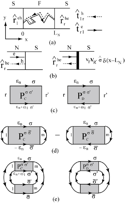
Figure 14: (a): a propagation process of a quasiparticle in a SFS junction. We describe the Andreev reflection coefficients in Eq. (44) by those at an ideal normal-metal/superconductor interface as shown in (b). (c): Cooperon and diffuson propagator. The diagrams for Josephson current (d) and its fluctuations (e).

In Fig 14(e), we show two typical diagrams for fluctuations. Not only $P^{\sigma\bar{\sigma}}$ but also $P^{\sigma{\sigma}}$ contributes to fluctuations. The Cooperon $P^{\sigma\bar{\sigma}}$ behaves like $e^{-L_{N}/\xi_{h}}$ similar to the Josephson current. On the other hand, $P^{\sigma{\sigma}}\sim e^{-L_{N}/\xi_{T}}$. Thus amplitude of fluctuations in SFS junctions is almost the same as that in SNS junctions. Our approach, however, is not suitable for calculating fluctuations because a number of diagrams contributes to fluctuations in addition to Fig. 14(e). Here we present the result for SNS junctions at $T=0$ and $\varphi=\pi/2$ obtained by a slightly different approach koyama

$$\delta J=\sqrt{\frac{\pi}{6}}eE_{Th}\sqrt{\frac{W}{L_{N}}}.$$ (73)

The fluctuations in SFS junctions are given by $\delta J/\sqrt{2}$ because contribution of $P^{\sigma,\bar{\sigma}}$ is negligible for $V_{ex}\gg E_{Th}$. Thus the ratio is described by

$$\frac{\delta J}{\langle J\rangle}\sim\frac{\sqrt{6\pi^{3}}}{16}\sqrt{\frac{L_{N}}{W}}\frac{1}{k_{F}\ell}{e^{L_{N}/\xi_{h}}}\frac{E_{Th}^{3/2}}{\Delta_{0}\sqrt{V_{ex}}}.$$ (74)

Since $P^{\sigma{\sigma}}\sim e^{-L_{N}/\xi_{T}}$, temperature dependence of fluctuations is also expected to be $e^{-L_{N}/\xi_{T}}$. Thus we arrive at Eq. (37). In a recent paper, mesoscopic fluctuations of the Josephson current were calculated within the quasiclassical Green function technique houzet2 . In this approach the fluctuations are slightly larger than those within the diagrammatic expansion altshuler ; koyama . The difference may stem from the proximity effect on electronic structure in a normal metal such as the minigap in the quasiparticle density of states. In the diagrammatic expansion, such effect is not taken into account.

Appendix B negative Josephson coupling

Here we express the Josephson current in S/HM/S junctions with spin-active interface on the basis of the diagrammatic expansion. In a half metal, we assume that the magnetic moment is parallel to $\boldsymbol{e}_{3}$. Thus transmission coefficients of an electron become

$$\hat{t}^{e}_{rl}=\frac{\hat{\sigma}_{0}+\hat{\sigma}_{3}}{2}t^{e}_{rl}(\uparrow)$$ (75)

because electric structure for $\downarrow$ spin is insulating in a half metal. Transmission coefficients of a hole are defined in the same way by $e\to h$. Andreev reflection coefficients $\hat{r}_{r}^{he}$ and $\hat{r}_{r}^{eh}$ in Eq. (44) are calculated at a normal-metal/ superconductor interface at which a spin-flip potential $v_{F}\boldsymbol{V}_{R}\cdot\hat{\boldsymbol{\sigma}}\delta(x-L_{N})$ is introduced as shown in the right figure of Fig. 14(b). Andreev reflection coefficients $\hat{r}_{l}^{he}$ and $\hat{r}_{l}^{eh}$ are also calculated at a normal-metal/ superconductor interface at which a spin-flip potential $v_{F}\boldsymbol{V}_{L}\cdot\hat{\boldsymbol{\sigma}}\delta(x)$ is considered. We assume that $\boldsymbol{V}_{L(R)}=\sum_{k=1}^{3}V_{L(R)}^{(k)}\boldsymbol{e}_{k}$ and $|\boldsymbol{V}_{L}|=|\boldsymbol{V}_{R}|=V_{S}$. The calculated results of Andreev reflection coefficients are given by

$$\hat{r}^{he}_{l}= -Q_{l}\hat{\sigma}_{2}\left[A_{l}\hat{\sigma}_{0}+iB_{l}\boldsymbol{V}_{L}\cdot\hat{\boldsymbol{\sigma}}\right]e^{-i\varphi_{L}},$$ (76)

$$\hat{r}^{eh}_{l}= Q_{l}\left[A_{l}\hat{\sigma}_{0}+iB_{l}\boldsymbol{V}_{L}\cdot\hat{\boldsymbol{\sigma}}\right]\hat{\sigma}_{2}e^{i\varphi_{L}},$$ (77)

$$Q_{l}= \frac{\Delta_{0}}{A_{l}^{2}+V_{S}^{2}B_{l}^{2}}\frac{q_{l}^{2}}{2},$$ (78)

$$A_{l}= -\Omega_{n}V_{S}^{2}+q_{l}^{2}\frac{(\Omega_{n}+\omega_{n})}{2},$$ (79)

$$B_{l}= q_{l}(\Omega_{n}+\omega_{n}),$$ (80)

where $q_{l}=k_{l}/k_{F}>0$ are normalized wave number of the $l$ th propagating channel in the current direction. Andreev reflection coefficients at the right interface $\hat{r}^{he}_{r}$ and $\hat{r}^{eh}_{r}$ are also obtained by $l\to r$, $\boldsymbol{V}_{L}\to\boldsymbol{V}_{R}$, and $\varphi_{L}\to\varphi_{R}$ in above expression. Since the half metal is in the diffusive transport regime, transmission coefficients across the half metal, namely $\hat{t}^{e}_{lr}$, $\hat{t}^{e}_{rl}$, $\hat{t}^{h}_{lr}$, and $\hat{t}^{h}_{rl}$ are independent of propagating channels $l$ and $r$. Thus average of the Andreev reflection coefficients over all propagating channels contribute to the Josephson current ya01-2 . We define such Andreev reflection coefficients as

$$\hat{r}^{he}_{l(r)}= \frac{1}{N_{c}}\sum_{l(r)}\hat{r}^{he}_{l(r)},$$ (81)

$$= -\hat{\sigma}_{2}\left[a\hat{\sigma}_{0}+ib\boldsymbol{V}_{L(R)}\cdot\hat{\boldsymbol{\sigma}}\right]e^{-i\varphi_{L(R)}},$$ (82)

$$\hat{r}^{eh}_{l(r)}= \frac{1}{N_{c}}\sum_{l(r)}\hat{r}^{he}_{l(r)},$$ (83)

$$= \left[a\hat{\sigma}_{0}+ib\boldsymbol{V}_{L(R)}\cdot\hat{\boldsymbol{\sigma}}\right]\hat{\sigma}_{2}e^{i\varphi_{L(R)}},$$ (84)

where $N_{c}=Wk_{F}/\pi$ is the number of propagating channels at Fermi energy, $a$ and $b$ are real numbers depending only on $\omega_{n}$, $\Delta_{0}$, and $V_{S}$. A part of Eq. (44) becomes

$$I_{1}= \sum_{{l},{r}}\left\langle\textrm{Tr}[\hat{r}^{eh}_{l}\cdot\hat{t}^{h}_{lr}\cdot\hat{r}^{he}_{r}\cdot\hat{t}^{e}_{rl}]\right\rangle,$$ (85)

$$= -\sum_{{l},{r}}\left\langle t_{lr}^{h}(\uparrow)t_{rl}^{e}(\uparrow)\right\rangle\frac{e^{i\varphi}}{4}\textrm{Tr}\left[(a+ib\boldsymbol{V}_{R}\cdot\hat{\boldsymbol{\sigma}})\right.$$

$$\times\left.(\hat{\sigma}_{0}-\hat{\sigma}_{3})(a+ib\boldsymbol{V}_{L}\cdot\hat{\boldsymbol{\sigma}})(\hat{\sigma}_{0}+\hat{\sigma}_{3})\right],$$ (86)

$$= e^{i\varphi}b^{2}g_{N}\frac{\eta^{\uparrow\uparrow}}{\sinh\eta^{\uparrow\uparrow}}$$

$$\times \left[\boldsymbol{V}_{L}\cdot\boldsymbol{V}_{R}-{V}_{L}^{(3)}{V}_{R}^{(3)}+i\boldsymbol{e}_{3}\cdot(\boldsymbol{V}_{R}\times\boldsymbol{V}_{L})\right],$$ (87)

where we used Eq. (64). In the same way, we obtain

$$I_{2}= \sum_{{l},{r}}\left\langle\textrm{Tr}[\hat{r}^{eh}_{r}\cdot\hat{t}^{h}_{rl}\cdot\hat{r}^{he}_{l}\cdot\hat{t}^{e}_{lr}]\right\rangle,$$ (88)

$$= e^{-i\varphi}b^{2}g_{N}\frac{\eta^{\uparrow\uparrow}}{\sinh\eta^{\uparrow\uparrow}}$$

$$\times \left[\boldsymbol{V}_{L}\cdot\boldsymbol{V}_{R}-{V}_{L}^{(3)}{V}_{R}^{(3)}-i\boldsymbol{e}_{3}\cdot(\boldsymbol{V}_{R}\times\boldsymbol{V}_{L})\right].$$ (89)

As a result, the expression for the Josephson takes the form

$$\langle J\rangle\approx -J_{1}\left[\left(\boldsymbol{V}_{L}\cdot\boldsymbol{V}_{R}-{V}_{L}^{(3)}{V}_{R}^{(3)}\right)\sin\varphi\right.$$

$$\left.+\boldsymbol{e}_{3}\cdot(\boldsymbol{V}_{L}\times\boldsymbol{V}_{R})\cos\varphi\right],$$ (90)

$$J_{1}= 2{e}g_{N}T\sum_{\omega_{n}}\frac{\eta^{\uparrow\uparrow}}{\sinh\eta^{\uparrow\uparrow}}b^{2}>0.$$ (91)

The Josephson current is zero in the absence of spin-flip scattering at the interface (i.e., $\boldsymbol{V}_{L}=\boldsymbol{V}_{R}=0$). We note that the ratio ${\eta^{\uparrow\uparrow}}/{\sinh\eta^{\uparrow\uparrow}}$ rapidly decreases to zero for $\omega_{n}/E_{Th}\gg 1$, whereas $\omega_{n}$ dependence of $b$ is scaled by $\Delta_{0}$. For $E_{Th}\ll\Delta_{0}$, we find at $T=0$

$$J_{1}= \frac{7\zeta(3)}{\pi}eE_{Th}\;g_{N}b^{2},$$ (92)

$$b= \frac{1}{2}\int_{0}^{\pi/2}\!\!\!\!d\gamma\;\frac{\cos^{5}\gamma}{\left(V_{S}^{2}+\frac{1}{4}\right)\cos^{4}\gamma-V_{S}^{2}\cos^{2}\gamma+V_{S}^{4}}.$$ (93)

Although Eq. (90) describes well the dependence of the Josephson current on $\boldsymbol{V}_{L}$ and $\boldsymbol{V}_{R}$, it does not explain the nonmonotonic temperature dependence of the critical current shown in Fig. 11(b). This is because the proximity effect on the density of states in a half metal is not taken into account in the above estimate.

References

- (1) P. Fulde and R. A. Ferrell, Phys. Rev. 135, A550 (1964).
- (2) A. I. Larkin and Y. N. Ovchinnikov, Sov. Phys. JETP 20, 762 (1965).
- (3) A. I. Buzdin, L. N. Bulaevskii, and S. V. Panyukov, JETP Lett. 35, 179 (1982).
- (4) A. I. Buzdin, Rev. Mod. Phys. 77, 935 (2005).
- (5) V. T. Petrashov, V. N. Antonov, S. Maksimov, and R. Shaikhaidarov, JETP Lett. 59, 551 (1994).
- (6) F. S. Bergeret, A. F. Volkov, and K. B. Efetov, Phys. Rev. Lett. 86, 4096 (2001); Rev. Mod. Phys. 77, 1321 (2005).
- (7) A. Kadigrobov, R. I. Shekhter, and M. Jonson, Europhys. Lett. 54, 394 (2001).
- (8) V. V. Ryazanov, V. A. Oboznov, A. Yu. Rusanov, A. V. Veretennikov, A. A. Golubov, and J. Aarts, Phys. Rev. Lett. 86, 2427 (2001).
- (9) T. Kontos, M. Aprili, J. Lesueur, F. Genet, B. Stephanidis, and R. Boursier, Phys. Rev. Lett. 89, 137007 (2002).
- (10) A. A. Golubov, M. Yu. Kupriyanov, and E. I’ichev, Rev. Mod. Phys. 76, 411 (2004).
- (11) K. Usadel, Phys. Rev. Lett. 25, 507 (1970).
- (12) J. W. A. Robinson, S. Piano, G. Burnell, C. Bell, and M. G. Blamire, Phys. Rev. Lett. 97, 177003 (2006).
- (13) R. S. Keizer, S. T. B. Goennenwein, T. M. Klapwijk, G. Miao, G. Xiao, A. Gupta, Nature 439, 825 (2006).
- (14) Y. Asano, Y. Tanaka, and A. A. Golubov, Phys. Rev. Lett. 98, 107002 (2007).
- (15) V. Braude and Yu. V. Nazarov, Phys. Rev. Lett. 98, 077003 (2007).
- (16) M. Eschrig and T. Lofwander, cond-mat/0612533.
- (17) S. Takahashi, S. Hikino, M. Mori, J. Martinek, and S. Maekawa, Phys. Rev. Lett. 99, 057003 (2007); S. Hikino, S. Takahashi, M. Mori, J. Martinek and S. Maekawa, Physica C 463-465, 198 (2007).
- (18) M. Eschrig, J. Kopu, J. C. Cuevas, and G. Schon, Phys. Rev. Lett. 90, 137003 (2003).
- (19) B. Al’tshuler and B. Z. Spivak, Sov. Phys. JETP 65, 343 (1987).
- (20) A. Yu. Zyuzin, B. Spivak, and M. Hruska, Europhys. Lett. 62, 97 (2003).
- (21) P. G. de Gennes, Superconductivity of Metals and Alloys, (Benjamin, New York, 1966).
- (22) A. Furusaki, Physica B. 203, 214 (1994).
- (23) Y. Asano, Phys. Rev. B 63, 052512 (2001).
- (24) G. Eilenberger, Z. Phys. 214, 195 (1968).
- (25) In two-dimensional lattices, wave function of a quasiparticle is basically localized due to random impurity potential. In the present parameter choice, the localization length and the mean free path at are estimated about 90 and 6 lattice constant, respectively. We have confirmed that these values are not so much sensitive to . The present parameter choice enables us to study transport in the diffusive transport regime because a relation is satisfied. Effects of the localization on Josephson current are important when we choose ya02-4 .
- (26) Y. Asano, Phys. Rev. B 64, 014511 (2001); J. Phys. Soc. Jpn. 71, 905 (2002).
- (27) Y. Tanaka and A. A. Golubov, Phys. Rev. Lett. 98, 037003 (2007).
- (28) A. F. Volkov, F. S. Bergeret, and K. B. Efetov, Phys. Rev. Lett. 90, 117006 (2003).
- (29) After submission, we have learned of a recent paper by M. Houzet and A. I. Buzdin, (Phys. Rev. B 76, 060504(R) (2007)) which gives the same conclusion.
- (30) M. Fogelstrom, Phys. Rev. B 62, 11812 (2000).
- (31) T. Kontos, M. Aprili, J. Lesueur, and X. Grison, Phys. Rev. Lett. 86, 304 (2001).
- (32) T. Yokoyama, Y. Tanaka, and A. A. Golubov, Phys. Rev. B 72, 052512 (2005).
- (33) Y. Tanaka and S. Kashiwaya, Phys. Rev. B 70, 012507 (2004); Y. Tanaka, S. Kashiwaya, and T. Yokoyama, Phys. Rev. B 71, 094513 (2005).
- (34) Y. Tanaka, Y. Asano, A. A. Golubov, and S. Kashiwaya, Phys. Rev. B 72, 140503(R) (2005).
- (35) Y. Asano, Y. Tanaka, and S. Kashiwaya, Phys. Rev. Lett. 96, 097007 (2006).
- (36) Y. Asano, Y. Tanaka, A. A. Golubov, and S. Kashiwaya, Phys. Rev. Lett. 99, 067005 (2007).
- (37) Y. Tanaka and S. Kashiwaya, Phys. Rev. Lett. 74, 3451 (1995).
- (38) Y. Asano, Phys. Rev. B 66, 174506 (2002).
- (39) Y. Koyama, Y. Takane, and H. Ebisawa, J. Phys. Soc. Jpn. 66, 430 (1997).
- (40) Y. Asano, Phys. Rev. B 64, 224515 (2001).
- (41) M. Houzet and M. A. Skvortsov, arXiv:0704.3436.