“No Information Without Disturbance”:
Quantum Limitations of Measurement

Abstract

In this contribution I review rigorous formulations of a variety of limitations of measurability in quantum mechanics. To this end I begin with a brief presentation of the conceptual tools of modern measurement theory. I will make precise the notion that quantum measurements necessarily alter the system under investigation and elucidate its connection with the complementarity and uncertainty principles.

1 Introduction

It is a great honor and pleasure for me to contribute to this celebration of the scientific life work and achievements of Abner Shimony, from whom I have received much inspiration, personal encouragement and the gift of friendship in a decisive period of my scientific career. When I came to know Abner more closely, I was thrilled to realize the close agreement between our quantum mechanical world views; and ever since, when contemplating foundational issues, I found myself often wonder: “What would Abner say?”. I am proud to share with Abner one piece of work on an important item of “unfinished business”, a paper on the insolubility of the quantum measurement problem [3], which I hope may prove useful as a stepping stone towards resolving this problem. In this contribution I will address another area of concern to Abner, one that remains even when the measurement problem is suspended: quantum limitations of measurements.

By way of introduction of terminology and notation I briefly review the basic and most general probabilistic structures of quantum mechanics, encoded in the concepts of states, effects and observables; I then recall how these objects enter the modeling of measurements (Section 2).

This general framework of quantum measurement theory will then be used to obtain precise formulations and proofs of some long-disputed limitations of quantum measurements, such as the inevitability of disturbance and entanglement in a measurement, the impossibility of repeatable measurements for continuous quantities, and the incompatibility between conservation laws and the notion of repeatable sharp measurements (Section 3). In Section 4 the “classic” quantum limitations expressed by the complementarity and uncertainty principles are revisited. Appropriate operational measures of inaccuracy and disturbance for the formulation of quantitative trade-off relations for (joint) measurement inaccuracies and disturbances have been introduced in recent years; these will be discussed in Section 5.

I conclude with an outlook on open questions (Section 6).

2 Quantum Measurement Theory - Basic Concepts

2.1 States, effects and observables

Every quantum system is represented by a finite or infinite-dimensional, separable Hilbert space $\mathcal{H}$ over the complex field $\mathbb{C}$. States are described as positive operators $T$ of trace equal to one. The set of states $\mathcal{S(H)}$ is a convex subset of the real vector space of all self-adjoint trace-class operators. The role of a quantum state is to assign a probability to the outcome of any measurement; in other words, associated with every measurement with possible outcomes $\omega_{i}$, $i=1,2,\dots$, are mappings $\mathcal{E}_{i}:\mathcal{S(H)}\to[0,1]$ assigning the probabilities $\mathsf{p}_{T}(\omega_{i})\equiv\mathcal{E}_{i}(T)$. Since mixtures of states lead to the corresponding mixtures of probabilities, it follows that the mappings $\mathcal{E}_{i}$ are affine and hence extend uniquely to bounded positive linear mappings. Since the dual space of the trace class is isomorphic to the vector space of bounded operators, each $\mathcal{E}_{i}$ is of the form $\mathcal{E}_{i}(T)=\mathrm{tr}\left[{TE_{i}}\right]$, where $E_{i}$ is an operator satisfying $\mathbbm{O}\leq E_{i}\leq\mathbbm{1}$ (here $\mathbbm{1}$ denotes the identity operator). Such operators are called effects. The set of effects will be denoted $\mathcal{E(H)}$. The normalization of the probability distributions $\mathsf{p}_{T}$ ($\sum_{i}\mathsf{p}_{T}(\omega_{i})=1$) entails the condition

$$\sum_{i}E_{i}=\mathbbm{1}.$$ (1)

The mapping $\omega_{i}\mapsto E_{i}$ together with the property (1) is a (discrete) instance of a normalized positive-operator-valued measure (POVM), the general definition being that of an operator-valued mapping $X\mapsto E(X)$ with the following properties: (i) the domain consists of all elements $X$ of a $\sigma$-algebra $\Sigma$ of subsets of an outcome space $\Omega$; (ii) the operators $E(X)$ in the range are effects; (iii) the mapping is $\sigma$-additive (with infinite sums defined as weak limits): $E(\bigcup_{i}X_{i})=\sum_{i}E(X_{i})$ for any finite or countable family of mutually disjoint sets in $\Sigma$; (iv) $E(\Omega)=\mathbbm{1}$. POVMs are taken as the most general representation of an observable. In this contribution the measurable space of outcomes $(\Omega,\Sigma)$ will be $(\mathbb{R},\mathcal{B}(\mathbb{R}))$ or $(\mathbb{R}^{2},\mathcal{B}(\mathbb{R}^{2}))$, where $\mathcal{B}(\mathbb{R}^{n})$ denotes the Borel algebra of subsets of $\mathbb{R}^{n}$. The usual notion of observable is then recovered as the special case of a projection-valued measure (PVM) on $\mathcal{B}(\mathbb{R})$, which is nothing but the spectral measure associated with a selfadjoint operator. Observables represented are called PVMs sharp observables, all other POVMs are referred to as unsharp observables. The extreme case of a trivial observable arises when all the effects in its range are trivial, that is, of the form $E(X)=\lambda_{X}\mathbbm{1}$; the statistics associated with trivial effects and observables carries no information about the state.

2.2 Measurement schemes

Measurements are physical processes and as such they are subject to the laws of physics. In quantum mechanics, a measurement performed on an isolated object is described as an interaction between this object system and an apparatus system, both being treated as quantum systems. Being a macroscopic system, the apparatus will interact with a wider environment, but it is often convenient and sufficient to subsume the degrees of freedom of this “rest of the world” into the description of the apparatus.

The quantum description of a measurement is succinctly summarized in the notion of a measurement scheme, i.e., a quadruple $\mathcal{M}:=\langle\mathcal{H}_{\mathcal{A}},T_{\mathcal{A}},U,Z\rangle$, where $\mathcal{H}_{\mathcal{A}}$ is the Hilbert space of the apparatus (or probe) system, $T_{\mathcal{A}}$ the initial apparatus state, $U=U(t_{0},t_{0}+\Delta t):\mathcal{H}\otimes\mathcal{H}_{\mathcal{A}}\to\mathcal{H}\otimes\mathcal{H}_{\mathcal{A}}$ is the unitary operator representing the time evolution and ensuing coupling between the object system and apparatus during the period of measurement from time $t_{0}$ to $t_{0}+\Delta t$. Finally, $Z$ is the apparatus pointer observable, usually modeled as a sharp observable.

A schematic sketch of a measurement process is given in Figure 1 which is taken from [4]. Here $T$ and $T_{\mathcal{A}}$ denote the initial states of the object and apparatus, and $V(T\otimes T_{\mathcal{A}}):=UT\otimes T_{\mathcal{A}}U^{*}$ is the final state of the compound system after the measurement coupling has ceased. It is understood that upon reading an outcome, symbolized in the diagram with a discrete label $k$, the apparatus is considered to be describable in terms of a pointer eigenstate $T_{\mathcal{A},k}$, and this determines uniquely the associated final state $T_{k}$ of the object, as will be shown below.

The observable measured by such a scheme is determined by the pointer statistics for every object input state and is thus represented by a POVM $E$ that is unambiguously defined by the following probability reproducibility condition:

$$\mathrm{tr}\left[{UT\otimes T_{\mathcal{A}}U^{*}\,I\otimes Z(X)}\right]=:\mathrm{tr}\left[{T\,E(X)}\right]\equiv\mathsf{p}^{E}_{T}(X).$$ (2)

Here $X$ is any element of a $\sigma$-algebra $\Sigma$ of subsets of an outcome space $\Omega$. The positivity of the operators $E(X)$ in the range of the map $X\mapsto E(X)$ and the measure properties of this map follows from the fact that the maps $X\mapsto\mathsf{p}^{E}_{T}(X)$ are probability measures for every state $T$.

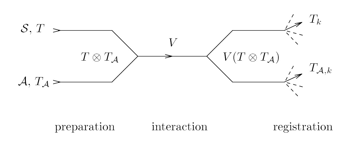
Figure 1: Sketch of a measurement scheme. The symbols are explained in the main body of the text.

The state $T_{X}$ of the object after recording a measurement outcome in the set $X$ is determined by the following sequential joint probability for a value of the pointer to be found in $X$ and an immediately subsequent measurement of an effect $B$ to yield a positive outcome:

$$\mathrm{tr}\left[{UT\otimes T_{\mathcal{A}}U^{*}\,B\otimes Z(X)}\right]=:\mathrm{tr}\left[{{\mathcal{I}}_{X}(T)\,B}\right]\equiv\mathrm{tr}\left[{T_{X}B}\right]$$ (3)

The maps $T\mapsto{\mathcal{I}}_{X}(T)=T_{X}$, called (quantum) operations, are affine and trace norm-nonincreasing:

$$\mathrm{tr}\left[{{\mathcal{I}}_{X}(T)}\right]=\mathrm{tr}\left[{T_{X}}\right]=\mathrm{tr}\left[{T\,E(X)}\right]\leq\mathrm{tr}\left[{T}\right]=1,$$ (4)

and they compose an instrument, that is, an operation-valued map $X\mapsto{\mathcal{I}}_{X}$. Note that these maps ${\mathcal{I}}_{X}$ extend in a unique way to linear maps on the complex vector space of trace class operators. The above equation shows that every instrument defines a unique POVM.

An important property of the operations ${\mathcal{I}}_{X}$ deriving from a measurement scheme is their complete positivity: for every $n\in\mathbb{N}$, the linear map defined by $T\otimes\Theta\mapsto{\mathcal{I}}_{X}(T)\otimes\Theta$ (where $T$ is any trace class operator on $\mathcal{H}$ and $\Theta$ is any trace class operator on $\mathbb{C}^{n}$) is positive, that is, it sends state operators to (generally non-normalized) state operators. The instrument composed of the completely positive operations is also called completely positive.

Every measurement scheme defines thus a unique completely positive instrument, and the latter fixes a unique POVM which represents the observable measured by the scheme. Starting from ground-breaking mathematical work of Neumark and Stinespring, the converse statement was developed in increasing generality by Ludwig and collaborators, Davies and Lewis, and Ozawa (detailed references can be found in [4]):

Theorem 1 (Fundamental Theorem of Quantum Measurement Theory).

Every observable, represented as a POVM $E$, admits infinitely many completely positive instruments ${\mathcal{I}}$ from which it arises via Eq. (2), and every completely positive instrument admits infinitely many implementations by means of a measurement scheme according to Eq. (3).

2.3 Examples

Next I recall some model realizations of measurement schemes and completely positive instruments; these will provide valuable case studies in subsequent sections.

2.3.1 Von Neumann model of an unsharp position measurement

On the final pages of his famous book of 1932, “Mathematische Grundlagen der Quantenmechanik”, von Neumann introduces a mathematical model of what he describes as a measurement of the position of a particle in one spatial dimension. Both the particle and measurement probe are represented by the Hilbert spaces $\mathcal{H}=\mathcal{H}_{\mathcal{A}}=L^{2}(\mathbb{R})$; and the coupling

$$U=\exp(-\tfrac{i}{\hbar}\lambda Q\otimes P_{\mathcal{A}}),$$ (5)

generates a correlation between the observable intended to be measured, $\mathsf{Q}$, and the pointer observable $Z=\mathsf{P}_{\mathcal{A}}$. To simplify the calculations, one assumes that the interaction is impulsive, that is, the coupling constant is large so that the duration of the interaction can be kept small enough so as to neglect the free Hamiltonians of the two systems. It is further assumed that the initial state of the probe is a pure state, $T_{\mathcal{A}}=P[\phi]$, with $\langle Q_{\mathcal{A}}\rangle_{\phi}:=\langle{\phi}|{Q_{\mathcal{A}}\phi}\rangle=0$ and finite variance $\mathrm{Var}(Q_{\mathcal{A}},\phi)=\langle Q_{\mathcal{A}}^{2}\rangle_{\phi}-\langle Q_{\mathcal{A}}\rangle_{\phi}^{2}$.

Von Neumann proceeded to calculate the correlation between the particle’s position and the pointer observable after the coupling period and took this measure of repeatability as an indication of the quality of the measurement. Had he made the computation associated with equation (2) above, he would have found the actually measured observable to be a smeared position observable $\mathsf{Q}_{e}$:

$$\begin{split}E=\mathsf{Q}_{e}:X\mapsto\mathsf{Q}_{e}(X)&=\chi_{X}*e(Q)=\int_{\mathbb{R}}\chi_{X}*e(q)\,\mathsf{Q}(dq),\\ \mathrm{where}\ e(q)&=\lambda|\phi(-\lambda q)|^{2}.\end{split}$$ (6)

Here $*$ denotes the convolution. Thus von Neumann was very close to discovering the representation of observables as POVMs! The variance $\mathrm{Var}(\mathsf{p}^{\mathsf{Q}_{e}}_{T})$ of the probability distribution $\mathsf{p}^{\mathsf{Q}_{e}}_{T}$ is

$$\mathrm{Var}(\mathsf{Q}_{e},T)=\int_{\mathbb{R}}(x-\overline{x})^{2}\mathsf{p}^{\mathsf{Q}_{e}}_{T}(dx)=\mathrm{Var}(\mathsf{Q},T)^{2}+\mathrm{Var}(e),$$ (7)

where $\overline{x}=\int_{\mathbb{R}}x\mathsf{p}^{\mathsf{Q}_{e}}_{T}(dx)=\mathrm{tr}\left[{TQ}\right]$. The second term in the expression for the variance, $\mathrm{Var}(e)$, indicates the unsharpness of the observable $\mathsf{Q}_{e}$ and at the same time is a measure of the inaccuracy of the measurement, that is, the separation between $\mathsf{Q}$ and $\mathsf{Q}_{e}$.

The instrument induced by von Neumann’s measurement scheme is given as follows:

$$\begin{split}{\mathcal{I}}^{\mathsf{Q}_{e}}:\,X,T\mapsto{\mathcal{I}}^{\mathsf{Q}_{e}}_{X}(T)&=\int_{X}K_{q}TK_{q}^{*}\,dq,\\ \mathrm{where}\ (K_{q}\varphi)(x)&=\sqrt{\lambda}\phi\left(\lambda(q-x)\right)\varphi(x).\end{split}$$ (8)

2.3.2 Ozawa’s model of a sharp position measurement

It turned out much more intricate to find a measurement scheme realizing a measurement of the sharp position observable. One solution was presented by Ozawa [5, 6] who introduced the following coupling:

$$\begin{split}U&=\exp\left[-\tfrac{i\pi}{3\sqrt{3}\hbar}(2Q\otimes P_{\mathcal{A}}-2P\otimes Q_{\mathcal{A}}+QP-Q_{\mathcal{A}}P_{\mathcal{A}})\right]\\ &=\exp\left(-\tfrac{i}{\hbar}Q\otimes P_{\mathcal{A}}\right)\,\exp\left(\tfrac{i}{\hbar}P\otimes Q_{\mathcal{A}}\right).\end{split}$$ (9)

Taking the pointer as $Z=\mathsf{Q}_{\mathcal{A}}$, the measured observable is $\mathsf{Q}$, the sharp position, independently of the choice of initial probe state $T_{\mathcal{A}}$. Indeed, the associated instrument is found to be

$${\mathcal{I}}^{\mathrm{Ozawa}}_{X}(T)=\int_{X}\mathrm{tr}\left[{T\mathsf{Q}(dq)}\right]\,e^{-\frac{i}{\hbar}qP}\,T_{\mathcal{A}}\,e^{\frac{i}{\hbar}qP},$$ (10)

so that $\mathrm{tr}\left[{TE(X)}\right]=\mathrm{tr}\left[{{\mathcal{I}}^{\mathrm{Ozawa}}_{X}(T)}\right]=\mathrm{tr}\left[{T\mathsf{Q}(X)}\right]$ for all states $T$ of the system.

3 Quantum Limitations on Measurability

The formalism of quantum measurements reviewed above provides a framework for the rigorous formulation of limitations on the measurability of physical quantities arising from quantum structures.

3.1 “No Information Gain Without Disturbance”

There has been much debate over the claim that according to quantum theory, every measurement necessarily “disturbs” the object system. Here is a theorem that states a precise sense in which this claim is true.

Theorem 2.

There is no instrument that leaves unchanged all states of the system unless the associated observable is trivial. More precisely: if an instrument ${\mathcal{I}}$ on $(\Omega,\Sigma)$ satisfies ${\mathcal{I}}_{\Omega}(T)=T$ for all $T\in\mathcal{S(H)}$, then $T\mapsto\mathrm{tr}\left[{{\mathcal{I}}_{X}(T)}\right]=:\lambda(X)$ is a constant map for all $X\in\Sigma$, and so the induced observable $E$ is trivial, $E(X)=\lambda(X)\mathbbm{1}$.

The proof is quickly sketched: if $T=P[\varphi]\mapsto{\mathcal{I}}_{\Omega}(P[\varphi])={\mathcal{I}}_{X}(P[\varphi])+{\mathcal{I}}_{\Omega\setminus X}(P[\varphi])=P[\varphi]$, then ${\mathcal{I}}_{X}(P[\varphi])=\lambda(X)P[\varphi]$. Due to the linearity of ${\mathcal{I}}_{X}$, the term $\lambda(X)$ is independent of $\varphi$, and the measured observable $E$ gives probabilities independent of $\varphi$: $\mathsf{p}^{E}_{\varphi}(X)=\mathrm{tr}\left[{{\mathcal{I}}_{X}(P[\varphi])}\right]=\lambda(X)$. QED

Hence a measurement scheme with no state change yields no information gain. We note that “disturbance” has here been interpreted as state change. This conclusion immediately leads to another question: is it possible to restrict the quality or accuracy of a measurement and thereby control the extent of the disturbance? This will be addressed in Section 5.

3.2 “No measurement without (some transient) entanglement”

It is a general fact of quantum mechanics that interactions between two systems lead to entanglement between them, that is, to states which are not of product form. From this it would seem to follow that in a measurement the object system and apparatus end up necessarily in an entangled state at the end of the coupling period. The next theorem shows that this implication does not hold true without qualifications.

Theorem 3.

Let $U:\mathcal{H}_{1}\otimes\mathcal{H}_{2}\rightarrow\mathcal{H}_{1}\otimes\mathcal{H}_{2}$ be a non-entangling unitary measurement coupling such that for a fixed vector $\phi_{0}$ and all vectors $\varphi\in\mathcal{H}_{1}$, one has $U(\varphi\otimes\phi)=\varphi^{\prime}\otimes\phi^{\prime}$. Then $U$ acts in the following way:
(a) $U(\varphi\otimes\phi_{0})=V(\varphi)\otimes\phi^{\prime}$, where $V$ is an isometry;
(b) $U\left(\varphi\otimes\phi_{0}\right)=\varphi^{\prime}\otimes W_{12}\varphi$, where $W_{12}:\mathcal{H}_{1}\rightarrow\mathcal{H}_{2}$ is a surjective isometry and $\varphi^{\prime}$ is a fixed vector in $\mathcal{H}_{1}$.

The proof is given in [7]. From this result it follows that if one aims at constructing a measurement scheme that leaves the object and apparatus in a non-entangled (separable) state after the coupling, and if this measurement is to transfer information about the initial object state $\varphi$ to the apparatus, then the coupling $U$ must act as in (b). It is therefore conceivable that after a suitable coupling interaction has been applied, the object and apparatus are left in an non-entangled state and yet complete information about the object state has been transferred to the apparatus. However, due to the continuity of the unitary dynamical evolution $t\mapsto U_{t}$ which comprises the coupling operator $U_{t+\Delta t}$, not all $U_{t^{\prime}}$ with $t<t^{\prime}<t+\Delta t$ can be of the non-entangling form (b), since that operator is not continuously connected with the identity operator $U_{0}$ at $t=0$. It follows that that some intermittent entanglement must build up during the interval $[t,t+\Delta t]$.

In order to extend this proof to measurement schemes for which the initial apparatus state$T_{\mathcal{A}}$ is not pure, it is necessary to sharpen the no-entanglement condition of the theorem to hold for any vector in $\mathcal{H}_{\mathcal{A}}$ whose projection operator can arise as a convex component of $T_{\mathcal{A}}$. These vectors are known to be given exactly by those in the range of $T_{\mathcal{A}}^{1/2}$ [8]. The following theorem, also proven in [7], can then be applied to take a step towards extending the above discussion to mixed apparatus states.

Theorem 4.

Let $U:\mathcal{H}_{1}\otimes\mathcal{H}_{2}\rightarrow\mathcal{H}_{1}\otimes\mathcal{H}_{2}$ be a unitary mapping such that for all vectors $\varphi\in\mathcal{H}_{1}$, $\phi\in\mathcal{H}_{2}$, the image of $\mathcal{H}_{1}\otimes\mathcal{H}_{2}$ under $U$ is of the form $U(\varphi\otimes\phi)=\varphi^{\prime}\otimes\phi^{\prime}$. Then $U$ is one of the following:
(A) $U=V\otimes W$ where $V:\mathcal{H}_{1}\rightarrow\mathcal{H}_{1}$ and $W:\mathcal{H}_{2}\rightarrow\mathcal{H}_{2}$ are unitary;
(B) $U\left(\varphi\otimes\phi\right)=V_{21}\phi\otimes W_{12}\varphi$, where $V_{21}:\mathcal{H}_{2}\rightarrow\mathcal{H}_{1}$ and $W_{12}:\mathcal{H}_{1}\rightarrow\mathcal{H}_{2}$ are surjective isometries.
The latter case can only occur if $\mathcal{H}_{1}$ and $\mathcal{H}_{2}$ are Hilbert spaces of equal dimensions.

It is not hard to construct a measurement scheme with a non-entangling coupling of the form (B) for any object observable $E$. This can be achieved by making the object interact with another system of the same type onto which the state of the original system is identically copied.

Example 1.

Let $\mathcal{H}_{1}=\mathcal{H}_{2}=\mathcal{H}$. Let $E:\Sigma\rightarrow\mathcal{E(H)}$ be a POVM in $\mathcal{H}$. Define $U\left(\varphi\otimes\phi\right)=\phi\otimes\varphi$. Then we have

$$\langle U\varphi\otimes\phi|I\otimes E\left(X\right)U\varphi\otimes\phi\rangle=\langle\varphi|E\left(X\right)\varphi\rangle.$$ (11)

3.3 “No repeatable measurement for continuous observables”

3.3.1 Repeatability and ideality

A measurement and its associated instrument are called repeatable if the probability for obtaining the same result upon immediate repetition of the measurement is equal to one:

$$\mathrm{tr}\left[{{\mathcal{I}}_{X}\left({\mathcal{I}}_{X}(T)\right)}\right]=\mathrm{tr}\left[{{\mathcal{I}}_{X}(T)}\right]\quad\mathrm{for\ all}\ X\in\Sigma,\ T\in\mathcal{S(H)}.$$ (12)

A measurement of a discrete observable and its associated instrument is called ideal if it does not change any eigenstate; thus, if the state $T$ is such that a particular outcome is certain to occur, then an ideal instrument does not alter the state:

$$\mathrm{for\ all\ }T,k,\quad\mathrm{if\ }\mathrm{tr}\left[{TP_{k}}\right]=1\ \mathrm{then\ }{\mathcal{I}}_{k}(T)=T.$$ (13)

Examples of repeatable measurements are the von Neumann and Lüders measurements which will be defined next.

Let $A$ be an observable with discrete spectrum and associated spectral decomposition $A=\sum_{k}a_{k}P_{k}$. We allow the eigenvalues to have multiplicity greater than one, so that the spectral projections can be decomposed into a sum of orthogonal rank-1 projections: $P_{k}=\sum_{\ell}P[\varphi_{k\ell}]$. Then a von Neumann measurement is a measurement whose associated instrument has the form

$${\mathcal{I}}_{k}^{\mathrm{vN}}(T)=\sum_{\ell}P[\varphi_{k\ell}]TP[\varphi_{k\ell}].$$ (14)

A Lüders measurement is a measurement whose associated instrument is given by:

$${\mathcal{I}}_{k}^{\mathrm{L}}(T)=P_{k}TP_{k}.$$ (15)

Note that Lüders measurement are ideal but von Neumann measurements are not ideal if at least one eigenvalue is degenerate. The ideal measurements are uniquely characterized by the form of their instruments [4]:

Theorem 5.

Any ideal measurement of a discrete sharp observable is a Lüders measurement.

In particular, it follows that every ideal measurement is repeatable. A much deeper result is the following, conjectured by Davies and Lewis in 1970 [9] and proven by M. Ozawa in 1984 [10]. An observable $E$ on $(\Omega,\Sigma)$ is discrete if there is a countable subset of $N$ of $\Omega$ such that $E(N)=\mathbbm{1}$.

Theorem 6.

If a measurement of an observable $E$ is repeatable then $E$ is discrete.

I discuss briefly the implications of these results. First observe that the existence of ideal measurements enables the applicability of the famous reality criterion of Einstein, Podolsky and Rosen [11]:

“If, without in any way disturbing a system, we can predict with certainty (i.e., with probability equal to unity) the value of a physical quantity, then there exists an element of physical reality corresponding to that physical quantity.”

Since ideal measurements are repeatable, the associated observables must be discrete. Hence the EPR criterion can only be applied to discrete observables or discrete coarse-grainings of continuous observables.

3.3.2 Approximate repeatability

While strict repeatability is impossible for continuous observables such as position (or momentum), there do exist instruments for position (say) that are approximately repeatable in the following sense. Let $\delta>0$, and for any (Borel) subset $X$ of $\mathbb{R}$ let $X_{\delta}$ denote the set of all points which have a distance of not more than $\delta$ from some point in $X$. (Since $X_{\delta}=\bigcup_{x\in X}[x-\delta,x+\delta]$, this set $X_{\delta}$ is a Borel set.) An instrument ${\mathcal{I}}$ on $\mathcal{B}(\mathbb{R})$ is $\delta$-repeatable if for all states $T$ and all $X\in\mathcal{B}(\mathbb{R})$,

$$\mathrm{tr}\left[{{\mathcal{I}}_{X_{\delta}}({\mathcal{I}}_{X}(T))}\right]=\mathrm{tr}\left[{{\mathcal{I}}_{X}(T)}\right].$$ (16)

An example is given by Ozawa’s instrument of a sharp position measurement, Eq. (10) if the probe state $T_{\mathcal{A}}$ is chosen such that its position distribution $\mathsf{p}_{T_{\mathcal{A}}}^{\mathsf{Q}_{\mathcal{A}}}$ is concentrated within $[-\delta,\delta]$.

The same form of instrument can also be defined for an unsharp position observable $\mathsf{Q}_{e}$,

$${\mathcal{I}}_{X}^{\mathsf{Q}_{e}}(T)=\int_{X}\mathrm{tr}\left[{T\mathsf{Q}_{e}(dq)}\right]e^{-iqP}T_{\mathcal{A}}e^{iqP},$$ (17)

and if $T$ is chosen as before, one can find $d>0$ such that

$$\mathrm{tr}\left[{{\mathcal{I}}_{X_{d}}^{\mathsf{Q}_{e}}({\mathcal{I}}_{X}^{\mathsf{Q}_{e}}(T))}\right]\geq(1-\varepsilon)\mathrm{tr}\left[{{\mathcal{I}}_{X}^{\mathsf{Q}_{e}}(T)}\right].$$ (18)

Instruments with this property can be called $(d,1-\varepsilon)$-repeatable. A detailed proof can be found in [12], and connections with the intrinsic unsharpness of the observable $\mathsf{Q}_{e}$ have recently been studied in [13].

3.3.3 Approximate ideality

Ideality is a form of nondisturbance, but it is restricted to the eigenstates of the measured observable: if the quantity being measured has a definite value, then such measurements do not change the state. But any state other than an eigenstate will be disturbed: it will be transformed into one of the eigenstates due to the repeatability property of an ideal measurement.

The tight link between ideality and repeatability is relaxed if unsharp observables are considered: these still allow a notion of approximate ideality, but that does not imply approximate repeatability. I illustrate the last statement by means of the generalized Lüders instrument associated with a discrete observable $E:\omega_{i}\mapsto E_{i}$:

$${\mathcal{I}}^{\mathrm{L}}_{i}(T)=E_{i}^{1/2}TE_{i}^{1/2}.$$ (19)

The operations ${\mathcal{I}}^{\mathrm{L}}_{i}$ have the following property:

$$\mathrm{if}\ \mathrm{tr}\left[{TE_{i}}\right]\geq 1-\varepsilon\ \mathrm{then\ }\mathrm{tr}\left[{{\mathcal{I}}^{\mathrm{L}}_{i}(T)E_{i}}\right]\geq(1-\varepsilon)\mathrm{tr}\left[{TE_{i}}\right].$$ (20)

That is, they do not decrease the probability. Further, it can be shown that for all states $T$ for which $\mathrm{tr}\left[{TE_{i}}\right]\geq 1-\varepsilon$, the (trace norm) difference between the states $T$ and ${\mathcal{I}}^{\mathrm{L}}_{i}(T)$ is of the order $\varepsilon^{1/2}$; this is the sense in which the generalized Lüders instruments are approximately ideal. Approximately ideal measurements enable a weakening of the EPR criterion applicable to unsharp or continuous observables, thus yielding a notion of unsharp reality [14].

It is not hard to construct examples of effects (with some eigenvalues small) such that the associated Lüders operation does not increase the small probability represented by that eigenvalue since the corresponding eigenstate is left unchanged. This shows that repeatability does not hold even in an approximate sense. Thus unsharp observables sometimes admit measurements that are less invasive than measurements of sharp observables.

The notion of a Lüders measurement was introduced by G. Lüders in 1951 [15] (english translation in [16]) who showed that such measurements can be used to test the compatibility of sharp observables.

Theorem 7 (Lüders Theorem).

Let $A=\sum_{k}a_{k}P_{k}$ and $B$ be two (discrete) observable. The following are equivalent:
(a) for all states $T$, $\mathrm{tr}\left[{\sum_{k}P_{k}BP_{k}}\right]=\mathrm{tr}\left[{TB}\right]$;
(b) $AB=BA$.

The statement also holds if the observable $B$ is not discrete or bounded; in that case statements (a) and (b) can be rephrased by replacing $B$ with all spectral projections of $B$. This theorem has been used in relativistic quantum theory to motivate the “local commutativity” condition by virtue of the postulate that measurements in one spacetime region should not lead to observable effects in another, spacelike separated region.

According to the Lüders theorem, any observable $B$ not commuting with $A$ is sensitive to a Lüders measurement being performed on $A$. In other words, a Lüders measurement of $A$ disturbs the distributions of $B$ in some states if $B$ does not commute with $A$. If $A,B$ are allowed to be unsharp observables, the corresponding statement is no longer true in general but requires stronger assumptions [17].

Theorem 8.

Let $E:\omega_{i}\mapsto E_{i}$ be a discrete observable and $B$ an effect. The following are equivalent if one of the assumptions (I) or (II) or (III) stated below holds:
(a’) for all states $T$, $\mathrm{tr}\left[{\sum_{k}E_{k}^{1/2}BE_{k}^{1/2}}\right]=\mathrm{tr}\left[{TB}\right]$;
(b’) $E_{k}B=BE_{k}$ for all $k$.
The assumptions are:
(I) $E$ is a simple observable with only two effects $E_{1},E_{2}=\mathbbm{1}-E_{1}$.
(II) $B$ has a discrete spectrum of eigenvalues that can be numbered in decreasing or increasing order.
(III) Condition (a’) is also stipulated for the effect $B^{2}$.

That some additional assumptions are necessary has been demonstrated by means of a counter example in [18]. There a discrete unsharp observable $E$ and effect $B$ not commuting with $E$ were found such that the generalized Lüders instrument of $E$ does not disturb the statistics of $B$.

3.4 Measurement limitations due to conservation laws

There is an obvious limitation on measurability due to the fact that the physical realization of a measurement scheme depends on the interactions available in nature. In particular, the Hamiltonian of any physical system has to satisfy the symmetry requirements associated with the fundamental conservation laws. This measurement limitation is reviewed in Abner Shimony’s contribution, so that here some complementary points and comments will be sufficient.

An early demonstration of the impact of the existence of additive conserved quantities on the measurability of a physical quantity was given by Wigner in 1952 [19]. Wigner showed that repeatable measurements of the $x$-component of a spin-1/2 system are impossible due to the conservation of the $z$-component of the total angular momentum of the system and the apparatus. The conclusion was generalized by other authors to the statement that a repeatable measurement of a discrete quantity is impossible if there is a (bounded) additive conserved quantity of the object plus apparatus system that does not commute with the quantity to be measured.

Wigner’s resolution was to show that a successful measurement can be realized with an angular-momentum-conserving interaction and with an arbitrarily high success probability if the apparatus is sufficiently large. Thus he allowed for an additional measurement “outcome” that indicated “no information” about the spin. The outcomes associated with “spin up” and “spin down” were shown to be reproduced with probabilities that came arbitrarily closely to the ideal quantum mechanical probabilities. In [20, Sec. IV.3] it was shown that this resolution amounts to describing the measurement by means of a POVM with three possible outcomes and associated effects $E_{+},E_{-},E_{?}$, where the effects $E_{\pm}=(1-\varepsilon)P^{s_{x}}_{\pm}$, i.e., they are “close to” the spectral projections of $s_{x}$ if $0<\varepsilon\leq 1$, and the effect $E_{?}=\varepsilon\mathbbm{1}$ is a multiple of $\mathbbm{1}$. It can be shown that $\varepsilon$ can be made very small if the size of the measuring system is large.

These considerations show that it is a matter of principle that measurements of spin can never be perfectly accurate as a consequence of the additive conservation law for total angular momentum. The the necessary inaccuracy is appropriately described by a POVM of the kind described above. However, the common description of a sharp spin measurement is found to be an admissible idealization; the error made by breaking (ignoring) the fundamental rotation symmetry of the measurement Hamiltonian is negligible due to the fact that the measuring system is very large.

It seems to be a difficult problem to decide whether a limitation of measurability arises also in cases where the observable to be measured and the conserved quantity are unbounded and have continuous spectra. This question was raised by Shimony and Stein in 1979 [21]. The most general result at that time was the following (expressed in the notation of the present paper):

Theorem 9.

If a sharp observable $E$ admits a repeatable measurement, and if $L\otimes\mathbbm{1}+\mathbbm{1}\otimes L_{\mathcal{A}}$ is a bounded selfadjoint operator representing a conserved quantity for the combined object and apparatus system, then $E$ commutes with $L$.

Since repeatable measurements exist only for discrete observables (Theorem 6), the above statement is only applicable to object observables with discrete spectra. Hence it does not apply to measurements of position.

Ozawa [22] presented what seems to be a counter example, using a coupling that is manifestly translation invariant. However, this model constitutes an unsharp position measurement which becomes a sharp measurement only if the initial state of the apparatus is allowed to be a non-normalizable state (that is, not a Hilbert space vector or state operator). A proof that a sharp position measurement (without repeatability, but with some additional physically reasonable assumptions) cannot be reconciled with momentum conservation was given in [23]. A general proof is still outstanding.

Here we use another modification of the von Neumann model to demonstrate that momentum conservation is compatible with unsharp position measurements where the inaccuracy can be made arbitrarily small [20, Sec. 4.3]. Note that the total momentum $P+P_{\mathcal{A}}$ commutes with the coupling

$$U=\exp\left(-i\tfrac{\lambda}{2}\bigl{[}(Q-Q_{\mathcal{A}})P_{\mathcal{A}}+P_{\mathcal{A}}(Q-Q_{\mathcal{A}})\bigr{]}\right).$$ (21)

The pointer is again taken to be $Z=\mathsf{Q}_{\mathcal{A}}$. Then the measured observable is the smeared position $\mathsf{Q}_{e}=e*\mathsf{Q}$, where $e(q)=\left(e^{\lambda}-1\right)\,\Bigl{|}\phi\bigl{(}-(e^{\lambda}-1)q\bigr{)}\Bigr{|}^{2}$.

One can argue that the clash between the conservation law and position measurement has been shifted and reappears when the measurement of $\mathsf{Q}_{\mathcal{A}}$ is considered. However, if momentum conservation is taken into account in the measurement of the pointer, it would turn out that the pointer itself is only measured approximately, that is, an unsharp pointer $\mathsf{Q}_{\mathcal{A},h}$ is actually measured, which then yields the measured observable as $\mathsf{Q}_{e*h}$.

The lesson of the current subsection is this: to the extent that the limitation on measurability due to additive conservation laws holds as a general theorem, it shows that the notion of a sharp measurement of the most important quantum observables is an idealization which can be realized only approximately as a matter of principle; yet the quality of the approximation can be extremely good due to the macroscopic nature of the measuring apparatus.

To conclude this section, it is worth remarking that the quantum limitations of measurements described here are valid independently of the view that one may take on the measurement problem. This is the case because these limitations follow from consideration of the total state of system and apparatus as it arises in the course of its unitary evolution.

4 Complementarity and Uncertainty

The “classic” expressions of quantum limitations of preparations and measurements are codified in the complementarity and uncertainty principles, formulated by Bohr and Heisenberg 80 years ago.

This section offers a “taster” for two recent extensive reviews on the complementarity principle, Ref. [24], and the uncertainty principle, Ref. [25], which together develop a novel coherent account of these two principles. In a nutshell, complementarity states a strict exclusion of certain pairs of operations whereas the uncertainty principle shows a way of “softening” complementarity into a graded, quantitative relationship, in the form of a trade-off between the accuracies with which these two options can be realized together approximately. This interpretation is compatible with, if not envisaged in, the following passage of Bohr’s published text of his famous Como lecture of 1927 [26].

“In the language of the relativity theory, the content of the relations (2) [the uncertainty relations] may be summarized in the statement that according to the quantum theory a general reciprocal relation exists between the maximum sharpness of definition of the space-time and energy-momentum vectors associated with the individuals. This circumstance may be regarded as a simple symbolical expression for the complementary nature of the space-time description and claims of causality. At the same time, however, the general character of this relation makes it possible to a certain extent to reconcile the conservation laws with the space-time co-ordination of observations, the idea of a coincidence of well-defined events in a space-time point being replaced by that of unsharply defined individuals within finite space-time regions.”

Bohr summarizes here his idea of complementarity as the falling-apart in quantum physics of the notions of observation, which leads to space-time description, and state definition, linked with conservation laws and causal description; he regarded the possibility of combining space-time description and causal description as an idealization that was admissible in classical physics. Note also the reference to unsharpness (the emphasis in the quotation is ours), which seems to constitute the first formulation of an intuitive notion of unsharp reality (and the first occurrence of this teutonic addition to the English language).

4.1 The Complementarity Principle

In a widely accepted formulation, the Complementarity Principle is the statement that there are pairs of observables which stand in the relationship of complementarity. That relationship comes in two variants, stating the mutual exclusivity of preparations or measurements of certain pairs of observables. In quantum mechanics there are pairs of observables the eigenvector basis systems of which are mutually unbiased. This means that the system is in an eigenstate of one observable, so that the value of that observable can be predicted with certainty, the values of the other observable are uniformly distributed. This feature is an instance of preparation complementarity, and it has been called value complementarity. Measurement complementarity of observables with mutually unbiased eigenbases can be characterized by the following property: any attempt to obtain simultaneous information about both observables by first measuring one and then the other is bound to fail since the first measurement completely destroys any information about the other observable; that is to say, the second measurement gives no information about the state prior to the first measurement. This will be illustrated in an example below. We conclude that the “principle” of complementarity, as formalized here, is in fact a consequence of the quantum mechanical formalism.

Examples of pairs of observables are spin-1/2 observables such as $s_{x},s_{z}$, and the canonically conjugate position and momentum observables $Q,P$ of a free particle. A unified formalization of preparation and measurement complementarity can be given in terms of the spectral projections of these observables ($P^{x}_{\pm},P^{z}_{\pm}$ for $s_{x},s_{z}$, and $\mathsf{Q}(X),\mathsf{P}(Y)$ for $Q,P$:

$$\begin{split}P^{x}_{k}\land P^{z}_{\ell}&=\mathbbm{O}\quad\mathrm{for\ }k,\ell=+,-\,;\\ \mathsf{Q}(X)\land\mathsf{P}(Y)&=\mathbbm{O}\quad\mathrm{for\ bounded\ intervals}\ X,Y.\end{split}$$ (22)

The symbol $\land$ represents the lattice-theoretic infimum of two projections, that is, for example, $\mathsf{Q}(X)\land\mathsf{P}(Y)$ is the projection onto the closed subspace which is the intersection of the ranges of $\mathsf{Q}(X)$ and $\mathsf{P}(Y)$. These relations entail, in particular, that complementary pairs of observables do not possess joint probability distributions associated with a state $T$ in the usual way: for example, there is no POVM $G:\mathcal{B}(\mathbb{R}^{2})\to\mathcal{E(H)}$ such that $G(X\times\mathbb{R})=\mathsf{Q}(X)$ and $G(\mathbb{R}\times Y)=\mathsf{P}(Y)$ for all $X,Y\in\mathcal{B}(\mathbb{R})$. In fact, if these marginality relations were satisfied for all bounded intervals $X,Y$, then one must have $G(X\times Y)\leq\mathsf{Q}(X)$ and $G(Y\times Y)\leq\mathsf{P}(Y)$, and this implies that any vector in the range of $G(X\times Y)$ must also be in the ranges of $\mathsf{Q}(X)$ and $\mathsf{P}(Y)$, hence $G(X\times Y)=\mathbbm{O}$.

Example 2 (Complementarity for measurement sequences (1)).

Let $A,B$ be observables in $\mathbb{C}^{n}$, $n\geq 2$, with mutually unbiased eigenbases $\varphi_{1},\varphi_{2},\dots,\varphi_{n}$ and $\psi_{1},\psi_{2},\dots,\psi_{n}$, respectively. (Hence $A,B$ are value complementary.) Let ${\mathcal{I}}^{A}$ be the repeatable (von Neumann-Lüders) instrument associated with $A$: ${\mathcal{I}}_{k}^{A}(T):=\langle{\varphi_{k}}|{T\varphi_{k}}\rangle|\varphi_{k}\,\rangle\langle\,\varphi_{k}|$. Let ${\mathcal{I}}_{\mathbb{R}}^{A}:=\sum_{k}{\mathcal{I}}^{A}_{k}$ be the nonselective measurement operation, then the probability for a $B$ measurement following the $A$ measurement is $\mathsf{p}^{B}_{{\mathcal{I}}_{\mathbb{R}}(T)}(\ell)=1/n$, which is independent of $T$. This can be expressed by saying that the observable effectively measured in this process is not $B$ but the trivial POVM whose effects are $E_{\ell}=\frac{1}{n}\mathbbm{1}$.

Example 3 (Complementarity for measurement sequences (2)).

Consider a measurement of position $Q$ followed by a measurement of momentum $P$. Let ${\mathcal{I}}^{\mathsf{Q}}$ be the instrument representing the position measurement. Then the following defines a joint probability distribution:

$$\mathrm{tr}\left[{{\mathcal{I}}^{\mathsf{Q}}_{X}(T)\,\mathsf{P}(Y)}\right]=\mathsf{p}_{T}(X\times Y)=:\mathrm{tr}\left[{TG(X\otimes Y)}\right],\quad X,Y\in\mathcal{B}(\mathbb{R}).$$ (23)

The marginal observables are sharp position and a “distorted momentum” observable, $G(X\times\mathbb{R})=\mathsf{Q}(X)$ and $G(\mathbb{R}\times Y)=\widetilde{\mathsf{P}}(Y)$. Since one of these marginal observables is a sharp observable, it follows that the effects of the other marginal observable commute with the sharp observable. But $\mathsf{Q}$ is a maximal observable, and so the effects $\widetilde{\mathsf{Q}}(Y)$ are in fact functions of the position operator. The attempted momentum measurement only defines an effectively measured observable which contains a “shadow” of the information of the first position measurement. Hence a sharp measurement of position destroys all prior information about momentum (and vice versa).

The following defines a completely positive instrument ${\mathcal{I}}^{\mathsf{Q}}$ which renders the effective observable defined by a subsequent momentum measurement trivial: let $T_{x}$ be the continuous family of positive operators of trace one, generated by $T_{x}:=U_{x}T_{0}U_{x}^{-1}$, where $U_{x}$ are unitary operators that commute with momentum $P$. Then put

$${\mathcal{I}}^{\mathsf{Q}}_{X}(T):=\int_{X}T_{x}\,\mathrm{tr}\left[{T\mathsf{Q}(dx)}\right].$$ (24)

The associated measured observable is indeed the sharp observable $\mathsf{Q}$ since $\mathrm{tr}\left[{{\mathcal{I}}^{\mathsf{Q}}_{X}(T)}\right]=\mathrm{tr}\left[{T\mathsf{Q}(X)}\right]$. Then the distorted momentum observable $\widetilde{\mathsf{P}}$ defined above is found to be:

$$\begin{split}\mathrm{tr}\left[{T\widetilde{\mathsf{P}}(Y)}\right]:=&\mathrm{tr}\left[{{\mathcal{I}}^{\mathsf{Q}}_{\mathbb{R}}(T)\mathsf{P}(Y)}\right]=\int_{\mathbb{R}}\mathrm{tr}\left[{T_{x}\mathsf{P}(Y)}\right]\mathrm{tr}\left[{T\mathsf{Q}(dx)}\right]\\ =&\int_{\mathbb{R}}\mathrm{tr}\left[{T_{0}U_{x}^{-1}\mathsf{P}(Y)U_{x}}\right]\mathrm{tr}\left[{T\mathsf{Q}(dx)}\right]\\ =&\int_{\mathbb{R}}\mathrm{tr}\left[{T_{0}\mathsf{P}(Y)}\right]\mathrm{tr}\left[{T\mathsf{Q}(dx)}\right]=\mathrm{tr}\left[{T_{0}\mathsf{P}(Y)}\right].\end{split}$$ (25)

Thus $\widetilde{\mathsf{P}}$ is a trivial observable. Note that in this calculation $\mathsf{Q}$ could have been replaced by any observable as the first-measured observable. However, if the instrument (24) is required to be approximately repeatable, then $T_{0}$ must have a position distribution concentrated around the origin 0, and $U_{x}$ must ensure that $T_{x}$ has a position distribution concentrated around the point $x$; this is achieved if $U_{x}$ is chosen to be $exp(\frac{i}{\hbar}xP)$. Notice that this form is in fact realized in the Ozawa instrument for a sharp position measurement,Eq. (10). While we have not shown that this form is necessary, this consideration suggests that for approximately repeatable position measurements a subsequent momentum measurement leads to a (nearly) trivial observable as the distorted momentum.

4.2 The Uncertainty Principle

Following Ref. [24], we propose that the term uncertainty principle refers to the broad statement that there are pairs of observables for which a trade-off relationship pertains for the degrees of sharpness of the preparation or measurement of their values, such that a simultaneous or sequential determination of the values requires a nonzero amount of unsharpness (latitude, inaccuracy, disturbance). This gives rise to three variants of uncertainty relations, exemplified here for position and momentum: first there is the well-known inequality for the widths of the probability distributions of position and momentum in any quantum state that can be expressed in terms of the standard deviations,

$$\Delta(\mathsf{Q},T)\Delta(\mathsf{P},T)\geq\tfrac{1}{2}\hbar.$$ (26)

Second, one may consider a trade-off relation for the inaccuracies in any attempted joint measurement of position and momentum,

$$\delta(\widetilde{\mathsf{Q}},\mathsf{Q})\,\delta(\widetilde{\mathsf{P}},\mathsf{P})\geq C\hbar,$$ (27)

where the inaccuracies are to be defined appropriately as measures of the differences between the sharp position and momentum observables $\mathsf{Q},\mathsf{P}$ and their approximations $\widetilde{\mathsf{Q}},\widetilde{\mathsf{P}}$, respectively, which are to be measured jointly. Finally, there is a trade-off between the accuracy of an approximate measurement of position (momentum) and a necessary disturbance of the momentum (position) distribution:

$$\delta(\widetilde{\mathsf{Q}},\mathsf{Q})\,D(\widetilde{\mathsf{P}},\mathsf{P})\geq C\hbar,\quad\delta(\widetilde{\mathsf{P}},\mathsf{P})\,D(\widetilde{\mathsf{Q}},\mathsf{Q})\geq C\hbar,$$ (28)

where $D(\widetilde{\mathsf{Q}},\mathsf{Q})$ and $D(\widetilde{\mathsf{P}},\mathsf{P})$ denote appropriate measures of the disturbance of position and momentum, respectively.

Suitable measures of inaccuracy and disturbance which make the last two measurement uncertainty relations precise will be presented in Section 5. It thus turns out that similar to the complementarity principle, the uncertainty principle in its three manifestations is also a formal consequence of the noncommutativity of the observables in question. The term “principle” may still be used to highlight the fact that the uncertainty relations reflect an important nonclassical feature of quantum mechanics.

4.3 Complementarity versus uncertainty?

The reviews [24] and [25] propose a resolution of a long-standing controversy over the relationship, relative roles and interplay of the complementarity and uncertainty principles. This resolution will be briefly summarized here. As indicated in the introductory quote from Bohr (1928), the traditional view describes the uncertainty relations as a formal expression of the complementarity principle. However, as a quick survey of the research and textbook literature on quantum mechanics shows, this view has met with a considerable degree of uneasiness by many. Some authors consistently avoid any reference to complementarity while others play down the significance of the uncertainty relations, denying them the status of a principle which they reserve for complementarity.

Yet, in recent years there has been a shift of perspective which was indeed anticipated in the same quote of Bohr: complementarity is seen as a statement of the impossibility of jointly performing certain pairs of preparation or measurement procedures, whereas the role of the uncertainty principle is to quantify the degree to which an approximate reconciliation of these mutually exclusive options becomes a possibility. It seems that in this way a more balanced assessment has been achieved: compared to the view that emphasized complementarity over uncertainty, the positive role of the uncertainty relations as enabling joint determinations and joint measurements is now highlighted more prominently; and even though it is true (as shown in [24]) that the uncertainty relations entail the complementarity relations in a suitable limit sense, it is still appropriate to point out the strict mutual exclusivity of sharp value assignments which, after all, is the reason for the quest for an approximate reconciliation in the form of simultaneous but unsharp value assignments.

The principles of complementarity and uncertainty are extreme manifestations of the existence of noncommuting pairs of observables and of superpositions of states, which both entail fundamental limitations of the possibilities of preparing or measuring simultaneous sharp values of observables that do not commute. These limitations are consequences of a famous theorem of von Neumann which we summarize here as follows.

Theorem 10.

Let $A$ and $B$ be two sharp observables represented as selfadjoint operators. The following are equivalent:
(a) $A$ and $B$ possess a joint spectral representation (possibility of preparing joint sharp values).
(b) $A$ and $B$ possess a joint observable that defines joint probabilities for them (jointly measurability).
(c) $AB=BA$.

The reason for the long-standing debate over the superiority of either the complementarity principle or the uncertainty principle seems to lie in the fact that the features of complementarity and uncertainty are formally intertwined in Hilbert space quantum mechanics. It is only in the context of theoretical frameworks more abstract and general than quantum or classical theories that the logical relationships between complementarity and uncertainty postulates can be investigated; in such a generalized setting these postulates can in fact be used as principles within a set of axioms from which the Hilbert space framework of quantum mechanics can be deduced. As an example, we note the work of P. Lahti together with the late S. Bugajski, Ref. [27], who used appropriate formalizations of complementarity and the existence of von Neuman-Lüders measurements in the so-called convexity framework to derive Hilbert space quantum theory.

5 Inaccuracy and disturbance in quantum measurements

It remains to show how the above programmatic statement of the uncertainty principle for joint and sequential measurements can be made precise by appropriate measures of inaccuracy and disturbance. Such measures are also applicable in the analysis of the other quantum limitations of measurability discussed in Sec. 3.

First I will introduce the idea of an approximate joint measurement of two noncommuting quantities and present an operational definition of measurement error applicable to continuous observables such as position and momentum; the error measures for these observables obey a trade-off relation valid in any approximate joint measurements. Then I will show that a trade-off relation between the accuracy of a measurement and the disturbance of the distributions of an observable not commuting with the measured observable can be considered as an instance of a trade-off relation between the inaccuracies in an approximate joint measurement of two noncommuting observables.

5.1 Approximate joint measurements

A necessary criterion for the joint measurability of two observables is the existence of a joint probability distribution for every state $T$ in the usual quantum mechanical form. Von Neumann’s theorem entails that two noncommuting sharp observables such as position and momentum do not possess joint distributions (for all states). Hence these observables are not jointly measurable. However, for the joint measurability of pairs of unsharp observables, commutativity is not a necessary requirement. This suggests the following consideration: it should be possible to find two jointly measurable observables $M_{1},M_{2}$ on $\mathcal{B}(\mathbb{R})$ which are approximations, in a suitable sense, of position $\mathsf{Q}$ and momentum $\mathsf{P}$, respectively. Then a measurement of a joint observable $M$ on $\mathcal{B}(\mathbb{R}^{2})$ of $M_{1},M_{2}$ will be accepted as an approximate joint measurement of $\mathsf{Q},\mathsf{P}$ if the deviations of $M_{1}$ from $\mathsf{Q}$ and of $M_{2}$ from $\mathsf{P}$ are finite in some appropriate measure. This constellation is shown in Figure 2.

Figure 2: Idea of a joint approximate measurement of position $\mathsf{Q}$ and momentum $\mathsf{P}$, by means of an observable $M$ on $\mathcal{B}(\mathbb{R}^{2})$ whose marginals $M_{1}$ and $M_{2}$ are approximations of $\mathsf{Q}$ and $\mathsf{P}$, respectively.

Two tasks need to be addressed in order to complete the above program. First, one needs to introduce suitable operational measures of inaccuracy, that is, of the deviation between two observables defined on the same outcome space $(\Omega,\Sigma)$. Second, since we are interested in good joint approximations of noncommuting pairs of observables, the optimal approximators $M_{1},M_{2}$ must be expected to be noncommuting and hence unsharp observables in order to be jointly measurable; therefore, the problem arises to quantify the necessary degree of unsharpness required for the joint measurability given the finite “distance” of $M_{1},M_{2}$ from two noncommuting observables.

The definition of such measures of inaccuracy and unsharpness will in general depend on the type of outcome space. A variety of approaches for the case $(\mathbb{R},\mathcal{B}(\mathbb{R}))$ are analyzed in [25] and compared in detail in [28], and the case of discrete (qubit) observables is investigated in [29]. Here I will give a brief survey of notions applicable to the position-momentum case.

5.1.1 Standard error

The only known measure that is universally applicable to different types of outcome spaces (barring questions of domains of unbounded operators) is a quantity that may be called standard error as it is defined in terms of the first and second moments of the relevant operator measures, similar to the standard deviation. This seems to be the only measure of inaccuracy or error that has been in use in the literature over an extended period. Examples of its application in the formulation of uncertainty relations for joint measurements are the works of Appleby [30, 31], Hall [32], and Ozawa (e.g., [33, 34]).

For an observable $E$ on $\mathcal{B}(\mathbb{R})$, let $E[k]:=\int x^{k}E(dx)$ denote the $k^{th}$ moment operator of $E$ (defined on its natural domain $D(E[k]):=\{\varphi\in\mathcal{H}\,:\,\left|\int x^{k}\langle{\psi}|{E(dx)\varphi}\rangle\right|<\infty\ \mathrm{for\ all\ }\psi\in\mathcal{H}\}$ [35]). Assume $\mathcal{M}$ is a measurement scheme defining an observable $E$ on $\mathcal{B}(\mathbb{R})$ which is intended to approximate the sharp position $\mathsf{Q}$. Then a suggestive choice of measure of inaccuracy is

$$\varepsilon(Z,\mathsf{Q};T):=\mathrm{tr}\left[{UT\otimes P[\phi]U^{*}(\mathbbm{1}\otimes Z[1]-Q\otimes\mathbbm{1})^{2}}\right]^{1/2}.$$ (29)

This can be expressed in terms of the actually measured observable $E$:

$$\varepsilon(E,\mathsf{Q};T):=\left(\mathrm{tr}\left[{T(E[1]-Q)^{2}}\right]+\mathrm{tr}\left[{T(E[2]-E[1]^{2})}\right]\right)^{1/2}.$$ (30)

The inaccuracy in a momentum measurement is defined similarly. Ozawa proved the following universal uncertainty relation for the marginals $M_{1},M_{2}$ of an observable $M$ on $\mathcal{B}(\mathbb{R}^{2})$:

$$\varepsilon(M_{1},\mathsf{Q})\varepsilon(M_{2},\mathsf{P})+\varepsilon(M_{1},\mathsf{Q})\Delta(\mathsf{P},T)+\Delta(\mathsf{Q},T)\varepsilon(\mathsf{P},T)\geq\frac{1}{2}\hbar.$$ (31)

He noted that the first product term can be zero (this happens in Ozawa’s model of a sharp position measurement introduced above), and considers this to be a demonstration that the Heisenberg uncertainty principle for joint measurements of position and momentum and that for inaccuracy vs disturbance does not have the common form with a state-independent lower bound.

However, this way of reasoning ignores two crucial deficiencies in the definition of $\varepsilon(E,\mathsf{Q};T)$ as a measure of inaccuracy. First, the above uncertainty relation is not a statement solely about measurement inaccuracies since it depends on the preparation of the system. An appropriate definition of measurement inaccuracy should give an estimate of error which can be obtained without reference to the state of the measured object (which usually is unknown in a measurement). This point was observed by Appleby in 1998 who introduced what we propose to call the (global) standard error:

$$\varepsilon(E,\mathsf{Q}):=\sup_{T\in\mathcal{S(H)}}\left(\mathrm{tr}\left[{T(E[1]-Q)^{2}}\right]+\mathrm{tr}\left[{T(E[2]-E[1]^{2})}\right]\right)^{1/2}.$$ (32)

This quantity gives rise to a universal trade-off relation for joint measurement errors.

Theorem 11.

Let $M$ be an observable on $\mathcal{B}(\mathbb{R}^{2})$. Its marginals $M_{1},M_{2}$ obey the following:

$$\varepsilon(M_{1},\mathsf{Q})\varepsilon(M_{2},\mathsf{P})\geq\tfrac{1}{2}\hbar.$$ (33)

Appleby [31] gave a simple informal derivation. A rigorous proof is given in [28].

The second deficiency of the definition of $\varepsilon(E,\mathsf{Q};T)$ – and also of $\varepsilon(E,\mathsf{Q})$ – lies in the fact that this quantity cannot be estimated in terms of the measurements of $E$ and $\mathsf{Q}$ under consideration unless the operators $E[1]$ and $\mathsf{Q}$ commute so that they can be jointly measured to determine the expectation of the operator $(E[1]-\mathsf{Q})^{2}$. If $E[1]$ and $\mathsf{Q}$ do not commute then normally the squared difference operator does not commute with either of them and a third, quite different measurement is required to find its expectation value. This is to say that the standard error is not operationally significant, in general.

An interesting but very special subclass of measurements where this deficiency does not arise is the family of unbiased measurements, for which $E[1]=\mathsf{Q}$. In this case the standard error is given solely by the second term in Eq. (30), which is actually an operational measure of the intrinsic noise or unsharpness of the approximator $E$ of $\mathsf{Q}$ (see below).

5.1.2 A distance between observables on $\mathcal{B}(\mathbb{R})$

In 2004, R. Werner [36] introduced a distance $d(E,F)$ between two observables $E$ and $F$ on $\mathcal{B}(\mathbb{R})$ which is sensitive to the distance of the bulks of probability distributions $\mathsf{p}_{T}^{E}$ and $\mathsf{p}_{T}^{F}$, and he derived an uncertainty relation for position and momentum. Some definitions are required in order to present this result.

For any bounded continuous function $g$ on $\mathbb{R}$, one can define the operator $L(g,E):=\int_{\mathbb{R}}g(x)E(dx)$. The definition of $d(E,F)$ makes use of the set of (Lipshitz) functions $\Lambda:=\{g:\mathbb{R}\to\mathbb{R}\,:\,g\ \mathrm{bounded},\ |g(x)-g(y)\leq|x-y|\}$. Werner’s distance then is given as follows:

$$d(E,F):=\sup\big{\{}\,\|L(g,E)-L(g,F)\|\,:\,g\in\Lambda\big{\}}$$ (34)

Werner’s joint measurement uncertainty relation is stated as follows [36].

Theorem 12.

Let $M_{1},M_{2}$ be marginals of an observable $M$ on $\mathcal{B}(\mathbb{R}^{2})$. The distances $d(M_{1},\mathsf{Q})$ and $d(M_{2},\mathsf{P})$ obey the inequality

$$d(M_{1},\mathsf{Q})\,d(M_{2},\mathsf{P})\geq C\hbar.$$ (35)

Here the optimal constant $C$ is determined via $C\hbar=E_{0}^{2}/(4ab)$, where $E_{0}$ is the lowest (positive) eigenvalue of the operator $a|Q|+b|P|$ for some $a,b>0$. Its value is given by $C\approx 0.304745$.

This result constitutes the first universal joint measurement inaccuracy relation for operationally significant measures of inaccuracy. Moreover, the proof techniques used turn out to be applicable for quite different definitions of inaccuracy (see [37, 28]). The distance $d(E,F)$ is geometrically appealing and constitutes a natural choice due to its connection with the so-called Monge metric on the space of probability measures on $\mathcal{B}(\mathbb{R})$. However, from an experimenter’s perspective, it may be considered less appealing to be asked to estimate $d(E,F)$ by measuring differences of expectation values for $L(g,E)$ and $L(g,F)$, where $g$ runs through the set $\Lambda$ of Lipshitz functions.

5.1.3 Error bar width

A measure of measurement inaccuracy that would appear natural to an experimenter is the width of error bars, which is estimated in a process of calibration: the measurement scheme to be calibrated is fed with systems prepared with fairly sharply defined values of (say) the position observable. For each value, one estimates the spread of output values which gives a measure of the error bar width. If this measure is found to be bounded across all input values, the measurement will be considered to constitute a good approximation of the position observable to be measured. This consideration is captured in the following definitions.

Let $M_{1}$ be an observable on $\mathcal{B}(\mathbb{R})$ which is to approximate $\mathsf{Q}$. Let $J_{q;\delta}:=[q-\delta/2,q+\delta/2]$. By ${\mathcal{W}}_{\varepsilon_{1},\delta}({M_{1}},\mathsf{Q})$ I denote the inaccuracy, defined as the smallest interval width $w$ such that whenever the value of $\mathsf{Q}$ is certain to lie within an interval $J_{q;\delta}$, then the output distribution $\mathsf{p}_{\varphi}^{M_{1}}$ is concentrated to within $1-\varepsilon_{1}$ in $J_{q;w}$:

$$\begin{split}{\mathcal{W}}_{\varepsilon_{1},\delta}({M_{1}},\mathsf{Q}):=\inf\{w\,|\ &\text{for all\ }q\in\mathbb{R},\,\psi\in\mathcal{H},\\ &\text{if\ }\mathsf{p}^{\mathsf{Q}}_{\psi}(J_{q;\delta})=1\ \text{then\ }\mathsf{p}_{\psi}^{M_{1}}(J_{q;w})\geq 1-\varepsilon_{1}\}.\end{split}$$ (36)

The inaccuracy describes the range within which the input values can be inferred from the output distributions, with confidence level $1-\varepsilon$, given initial localizations within $\delta$. The inaccuracy is an increasing function of $\delta$, so that one can define the error bar width of $M_{1}$ relative to $\mathsf{Q}$:

$${\mathcal{W}}_{\varepsilon_{1}}({M_{1}},\mathsf{Q}):=\inf_{\delta}{\mathcal{W}}_{\varepsilon_{1},\delta}({M_{1}},\mathsf{Q})=\lim_{\delta\to 0}{\mathcal{W}}_{\varepsilon_{1},\delta}({M_{1}},\mathsf{Q}).$$ (37)

If ${\mathcal{W}}_{\varepsilon_{1}}({M_{1}},\mathsf{Q})$ is finite for all $\varepsilon_{1}\in(0,\frac{1}{2})$, we will say that $M_{1}$ approximates $\mathsf{Q}$ in the sense of finite error bars. Similar definitions apply to approximations $M_{2}$ of momentum $\mathsf{P}$, yielding ${\mathcal{W}}_{\varepsilon_{2},\delta}({M_{2}},\mathsf{P})$ and ${\mathcal{W}}_{\varepsilon_{2}}({M_{2}},\mathsf{P})$.

It is interesting to note that the finiteness of either $\epsilon(M_{1},\mathsf{Q})$ or $d(M_{1},\mathsf{Q})$ implies the finiteness of ${\mathcal{W}}_{\varepsilon_{1}}({M_{1}},\mathsf{Q})$ [28]. Therefore, among the three measures of inaccuracy introduced above, the condition of finite error bars gives the most general criterion for selecting “good” approximations of $\mathsf{Q}$ and $\mathsf{P}$.

The following uncertainty relation for error bar widths is proven in [37].

Theorem 13.

Let $M$ be an observable on $\mathcal{B}(\mathbb{R}^{2})$. The marginals $M_{1},M_{2}$ obey the following trade-off relation (for $0<\varepsilon_{1},\varepsilon_{2}<\frac{1}{2}$):

$${\mathcal{W}}_{\varepsilon_{1}}({M_{1}},\mathsf{Q})\,{\mathcal{W}}_{\varepsilon_{2}}({M_{2}},\mathsf{P})\geq 2\pi\left(1-\varepsilon_{1}-\varepsilon_{2}\right)^{2}\,\hbar.$$ (38)

5.1.4 Unsharpness

There are various measures of the intrinsic unsharpness of an observable $E$ on $\mathcal{B}(\mathbb{R})$. Here we briefly review a measure based on the noise operator of $E$, given by the positive operator $N(E):=E[2]-E[1]^{2}$. Note that this quantity appeared in the definition of the standard error, Eqs. (30), (32). The (intrinisic) noise is defined as

$$\mathcal{N}(E):=\sup_{T\in\mathcal{S(H)}}\mathrm{tr}\left[{T\,N(E)}\right]=\sup_{T\in\mathcal{S(H)}}\mathrm{tr}\left[{T\,(E[2]-E[1]^{2})}\right].$$ (39)

In the case where $E[1]$ is a selfadjoint (rather than only symmetric) operator, it is known that $N(E)=\mathbbm{O}$ if and only if $E$ is a sharp observable. The following trade-off relation for the noise in approximate joint measurements of position and momentum is proven in [28].

Theorem 14.

Let $M$ be an approximate joint observable for $\mathsf{Q},\mathsf{P}$ in the sense of finite error bars. Then the noise of $M_{1}$ and the noise of $M_{2}$ obey the following inequality:

$$\mathcal{N}(M_{1})\,\mathcal{N}(M_{2})\geq\tfrac{1}{2}\hbar.$$ (40)

An alternative measure of the intrinsic unsharpness of an observable on $\mathcal{B}(\mathbb{R})$ is given by the resolution width, introduced in [13]; this quantity is similar in spirit to the error bar width, and it is again found to yield a universal trade-off relation in joint measurements [28].

5.2 Inaccuracy-disturbance trade-off

We have seen that a momentum measurement following a sharp position measurement defines an observable that carries no information about the momentum distributions of the states prior to the position measurement. A sharp measurement of position thus destroys completely the momentum information contained in the initial state. The question arises whether the disturbance of momentum can be diminished if the position is measured approximately rather than sharply.

This possibility was already envisaged by Heisenberg in his discussion of thought experiments illustrating the uncertainty relations [38, 39]. For example, in the case of a particle passing through a slit he noted that due to the diffraction at the slit, an initially sharp momentum distribution is distorted into a broader distribution whose width $\Delta p$ is of the order $\hbar/\delta x$, where $\delta x$ is the width of the slit. The width $\Delta p$ is a measure of the change, or disturbance, of the momentum distribution, and $\delta x$ can be interpreted as the inaccuracy of the position determination effected by the slit. Further, one may also consider the recording of the location at which the particle hits the screen as a geometric determination of the (direction) of its momentum, the inaccuracy $\delta p$ of which is given by the width $\Delta p$ of the distribution obtained after many repetitions of the experiment. In this way the passage through the slit followed by the recording at the screen constitutes an approximate joint measurement of the position and momentum of the particle at the moment of its passage through the slit; see Figure 3.

Figure 3: Slit experiment as an approximate (sequential) joint measurement of position and momentum.

Generalizing this idea of making an approximate joint measurement by way of a sequence of approximate measurements, we consider the schemes of Figures 5 and 5). Here $M_{1}$ is either the sharp position $\mathsf{Q}$ or an unsharp position observable $\mathsf{Q}_{e}$ measured first, followed by a sharp momentum observable, whose measurement is to be followed by a sharp momentum measurement. The observable $M_{2}$ effectively measured by this momentum measurement is defined via $\mathsf{p}_{T}^{M_{2}}:=\mathsf{p}_{T^{\prime}}^{\mathsf{P}}$ for all initial states $T$, where $T^{\prime}$ is the state after the position measurement. Thus $M_{2}$ is the “distorted” momentum observable. Collecting the probabilities for finding an outcome in a set $X$ for the first measurement and an outcome in $Y$ for the second measurement defines a probability measure for each state $T$ via $X\times Y\mapsto\mathsf{p}_{T}(X\times Y)$. Hence there is a unique joint observable $M$ for $M_{1}$ and $M_{2}$ determined by the given measurement scheme [25].

In the first case, since the marginal $M_{1}=\mathsf{Q}$ is sharp, $M_{2}$ commutes with $\mathsf{Q}$ and is therefore not a good approximation of the momentum observable $\mathsf{P}$. However, in the second case, $M_{1}=\mathsf{Q}_{e}$, it is known [40] that the second marginal observable $M_{2}$ is a smeared momentum observable, $M_{2}=\mathsf{P}_{f}$, if the first, unsharp position measurement is such that the induced instrument is the von Neumann instrument (8). The inaccuracy distributions are then related as follows (cf. Eq. (6)):

$$e(q)=\lambda|\phi(-\lambda q)|^{2},\quad f(p)=\tfrac{1}{\lambda}|\widetilde{\phi}(-\tfrac{1}{\lambda}p)|^{2}.$$ (41)

Here $\widetilde{\phi}$ is the Fourier transform of $\phi$, from which it follows that the standard deviations of the distributions $e,f$ obey the uncertainty relation:

$$\Delta(e)\Delta(f)\geq\tfrac{1}{2}\hbar.$$ (42)

Note that $\Delta(e)$, $\Delta(f)$ are measures of how well the sharp observables $\mathsf{Q},\mathsf{P}$ are approximated by $M_{1},M_{2}$, respectively. Thus they are measures of measurement inaccuracy, and at the same time $\Delta(f)$ quantifies the disturbance of the momentum distribution due to the position measurement.

(1) $M_{1}=\mathsf{Q}$:

Figure 4: Sharp position measurement followed by a sharp momentum measurement. The two marginals $M_{1}=\mathsf{Q}$ and $M_{2}$ commute and have a unique joint observable $M$.

(2) :

Figure 5: Approximate joint measurement of position and momentum defined by an unsharp position measurement followed by a sharp momentum measurement. The marginals are $M_{1}=\mathsf{Q}_{e}$ and $M_{2}=\mathsf{P}_{f}$ where $e,f$ are probability distributions which are related as described in the main text.

These considerations show that an operational definition disturbance of the momentum distribution due to a position measurement is obtained by considering the sequential joint measurement composed of first measuring position and then momentum. The inaccuracy of the second measurement, that is, any measure of the separation between $\mathsf{P}$ and $M_{2}$, is also a measure of the momentum disturbance. Consequently, all the joint measurement inaccuracy relations discussed above apply to sequential joint measurements of position and momentum, and in this case they constitute rigorous versions of the long-sought-after inaccuracy-vs-disturbance trade-off relations.

6 Conclusion

Using the apparatus of modern quantum measurement theory, I have reviewed rigorous formulations of some well-known quantum limitations of measurements: the inevitability of disturbance and (transient) entanglement; the impossibility of repeatable measurements for continuous quantities, the restrictions on measurements arising from the presence of an additive conserved quantity, and the necessarily approximate and unsharp nature of joint measurements of noncommuting quantities.

In each case, a strict no-go theorem is complemented with a positive result describing conditions for an approximate realization of the impossible goal: repeatability can be approximated arbitrarily well for continuous sharp observables, also in the presence of a conservation law. It was found that ideal measurements of sharp observables are necessarily repeatable, but in the case of unsharp observables, approximate ideality can be achieved without forcing approximate repeatability. Thus, unsharp measurements may be less invasive than sharp measurements.

The impossibility of joint sharp measurements of complementary pairs of observables can be modulated into the possibility of approximate joint measurements of such observables, provided the inaccuracies are allowed to obey a universal Heisenberg uncertainty relation. Likewise, the complete destruction of momentum information by a sharp position measurement can be avoided if an unsharp position measurement is performed. The trade-off between the information gain in the approximate measurement of one observable and the disturbance of (the distribution of) its complementary partner observable was found to be an instance of the joint-measurement uncertainty relation.

These results, some of which were made precise in very recent investigations, open up a range of interesting new questions and tasks. In particular, it will be important to find operational measures of inaccuracy that are applicable to all types of observables, whether bounded or unbounded, discrete or continuous. This would probably enable a formulation of a universal form of joint measurement uncertainty relation for arbitrary pairs of (noncommuting) observables, thus generalizing the relations presented here for the special case of complementary pairs of continuous observables such as position and momentum.

Acknowledgement. This work was carried out during my visiting appointment at the Perimeter Institute (2005-2007). Hospitality and support by PI are gratefully acknowledged.

References

- [1]
- [2]
- [3] P. Busch and A. Shimony. Insolubility of the quantum measurement problem for unsharp observables. Stud. Hist. Phil. Mod. Phys., 27:397–404, 1996.
- [4] P. Busch, P.J. Lahti, and P. Mittelstaedt. The Quantum Theory of Measurement. Springer-Verlag, Berlin, second revised edition, 1996.
- [5] M. Ozawa. Measurement breaking the standard quantum limit for free-mass position. Phys. Rev. Lett., 60:385–388, 1988.
- [6] M. Ozawa. Position measuring interactions and the Heisenberg uncertainty principle. Phys. Lett A, 299:1–7, 2002.
- [7] P. Busch. The role of entanglement in quantum measurement and information processing. Int. J. Theor. Phys., 42(5):937–941, 2003.
- [8] N. Hadjisavvas. Properties of mixtures of non-orthogonal states. Lett. Math. Phys., 5:327–332, 1981.
- [9] E.B. Davies and J.T. Lewis. An operational approach to quantum probability. Comm. Math. Phys., 17:239–260, 1970.
- [10] M. Ozawa. Quantum measuring processes of continuous observables. J. Math. Phys., 25:79–87, 1984.
- [11] A. Einstein, B. Podolsky, and N. Rosen. Can quantum-mechanical description of physical reality be considered complete? Phys. Rev., 47:777–780, 1935.
- [12] P. Busch and P. Lahti. Some remarks on unsharp quantum measurements, quantum nondemolition, and all that. Ann. Physik, 47:369–382, 1990.
- [13] C. Carmeli, T. Heinonen, and A. Toigo. Intrinsic unsharpness and approximate repeatability of quantum measurements. J. Phys. A, 40:1303–1323, 2007.
- [14] P. Busch. Can quantum theoretical reality be considered sharp? In P. Mittelstaedt and E.W. Stachow (eds.), Recent Developments in Quantum Logic, Bibliographisches Institut, Mannheim, pp. 81–101, 1985.
- [15] G. Lüders. Über die Zustandsn̈derung durch den Meßprozeß. Annalen der Physik, 8:322–328, 1951.
- [16] G. Lüders. Concerning the state-change due to the measurement process. Ann. Phys. (Leipzig), 15(9):663–670, 2006.
- [17] P. Busch and J. Singh. Lüders theorem for unsharp quantum measurements. Phys. Lett. A, 249:10–12, 1998.
- [18] A. Arias, A. Gheondea, and S. Gudder. Fixed points of quantum operations. J. Math. Phys., 43(12):5872–5881, 2002.
- [19] E.P. Wigner. Die Messung quantenmechanischer Operatoren. Z. Phys., 133:101–108, 1952.
- [20] P. Busch, M. Grabowski, and P.J. Lahti. Operational Quantum Physics. Springer-Verlag, Berlin, 1997. second corrected printing.
- [21] A. Shimony and H. Stein. A Problem in Hilbert Space Theory Arising from the Quantum Theory of Measurement. Am. Math. Mon., 86:292–293, 1979.
- [22] M. Ozawa. Does a conservation law limit position measurements? Phys. Rev. Lett., 67(15):1956–1959, 1991.
- [23] P. Busch. Momentum conservation forbids sharp localisation. J. Phys. A: Math. Gen., 18:3351–3354, 1985.
- [24] P. Busch and C. Shilladay. Complementarity and uncertainty in Mach–Zehnder interferometry and beyond. Phys. Rep., 435:1–31, 2006.
- [25] P. Busch, T. Heinonen, and P.J. Lahti. Heisenberg’s uncertainty principle. Phys. Rep., in press, 2007.
- [26] N. Bohr. The quantum postulate and the recent development of atomic theory. Nature, 121:580–590, 1928.
- [27] P.J. Lahti and S. Bugajski. Fundamental principles of quantum theory. II. From a convexity scheme to the DHB theory. Int. J. Theor. Phys., 24:1051–1980, 1985.
- [28] P. Busch and D.B. Pearson. Inaccuracy and unsharpness in approximate joint measurements of position and momentum. In preparation, 2007.
- [29] P. Busch and T. Heinonen. Approximate joint measurements of qubit observables. arXiv:0706.1415, 2007.
- [30] D.M. Appleby. Concept of experimental accuracy and simultaneous measurements of position and momentum. Int. J. Theor. Phys., 37:1491–1509, 1998.
- [31] D.M. Appleby. Error principle. Int. J. Theor. Phys., 37:2557–2572, 1998.
- [32] M.J.W. Hall. Prior information: How to circumvent the standard joint-measurement uncertainty relation. Phys. Rev. A, 69:052113/1–12, 2004.
- [33] M. Ozawa. Universally valid reformulation of the Heisenberg uncertainty principle on noise and disturbance in measurement. Phys. Rev. A, 67:042105, 2003.
- [34] M. Ozawa. Uncertainty relations for noise and disturbance in generalized quantum measurements. Ann. Phys. (N.Y.), 311:350–416, 2004.
- [35] A. Dvurečenskij, P. Lahti, and K. Ylinen. Positive operator measures determined by their momentum sequences. Reports on Mathematical Physics, 45:139–146, 2000.
- [36] R.F. Werner. The uncertainty relation for joint measurement of position and momentum. Qu. Inf. Comp., 4:546–562, 2004.
- [37] P. Busch and D.B. Pearson. Universal joint-measurement uncertainty relation for error bars. J. Math. Phys., in press, 2007 (available at math-ph/0612074).
- [38] W. Heisenberg. Über den anschaulichen Inhalt der quantentheoretischen Kinematik und Mechanik. Z. Phys., 43:172–198, 1927.
- [39] W. Heisenberg. The Physical Principles of the Quantum Theory. University of Chicago Press, Chicago, 1930.
- [40] E.B. Davies. On the repeated measurements of continuous observables in quantum mechanics. J. Funct. Anal., 6:318–346, 1970.