Nonlinear elastic stress response in granular packings

Abstract

We study the nonlinear elastic response of a two-dimensional material to a localized boundary force, with the particular goal of understanding the differences observed between isotropic granular materials and those with hexagonal anisotropy. Corrections to the classical Boussinesq result for the stresses in an infinite half-space of a linear, isotropic material are developed in a power series in inverse distance from the point of application of the force. The breakdown of continuum theory on scales of order of the grain size is modeled with phenomenological parameters characterizing the strengths of induced multipoles near the point of application of the external force. We find that the data of Geng et al. Geng et al. (2001) on isotropic and hexagonal packings of photoelastic grains can be fit within this framework. Fitting the hexagonal packings requires a choice of elastic coefficients with hexagonal anisotropy stronger than that of a simple ball and spring model. For both the isotropic and hexagonal cases, induced dipole and quadrupole terms produce propagation of stresses away from the vertical direction over short distances. The scale over which such propagation occurs is significantly enhanced by the nonlinearities that generate hexagonal anisotropy.

I Introduction

The response of a granular medium to a localized boundary force has been investigated both experimentally and numerically Geng et al. (2001, 2003); Serero et al. (2001); Reydellet and Clément (2001); Mueggenburg et al. (2002); Spannuth et al. (2004); Head et al. (2001); Goldenberg and Goldhirsch (2004, 2005); Kasahara and Nakanishi (2004); Moukarzel et al. (2004); Gland et al. (2006); Ellenbroek et al. (2005, 2006); Ostojic and Panja (2005, 2006). Experiments have shown that in disordered packings stress response profiles consist of a single peak that broadens linearly with depth Geng et al. (2003); Serero et al. (2001). For hexagonal packings of disks Geng et al. (2001, 2003) or face-centered cubic packings of spheres Mueggenburg et al. (2002); Spannuth et al. (2004), on the other hand, the stress response develops multiple peaks that seem to coincide with propagation along lattice directions. In two dimensions, a hexagonal packing is indistinguihable from an isotropic one in the context of classical (linear) elasticity theory Boussinesq (1885); Otto et al. (2003). Thus the observation of response profiles in two-dimensional disordered and hexagonal packings that differ significantly on scales up to 30 grain diameters Geng et al. (2001, 2003) requires consideration of nonlinear effects. More generally, the applicability of classical elasticity to granular media is a question of ongoing research Ellenbroek et al. (2006); Wyart et al. (2005); Ball and Blumenfeld (2002); Goldenberg and Goldhirsch (2005); Tordesillas et al. (2004); Ostojic and Panja (2006).

Classical elasticity for an isotropic medium predicts a single-peaked pressure profile that broadens linearly with depth Boussinesq (1885). Numerical results (see Ref. Gland et al. (2006), for example) demonstrate responses well described by this solution in regions far from a localized force in the bulk of a disordered frictional packing with more than the critical number of contacts required for rigidity (the isostatic point). Recent work by Wyart Wyart et al. (2005) and Ellenbroek Ellenbroek et al. (2006) clarifies the onset of elastic behavior as average coordination number is increased above the isostatic limit. For materials with sufficiently strong uniaxial anisotropy, classical elasticity theory admits double-peaked profiles with both peak widths and the separation between peaks growing linearly as a function of depth Otto et al. (2003). The domain of applicability of classical elasticity theory to granular materials is not well understood, however, as it offers no simple way to incorporate noncohesive forces between material elements or history dependent frictional forces. Several alternative theories for granular stress response have been proposed that make predictions qualitatively different from conventional expectations. Models of isostatic materials Tkachenko and Witten (1999); Blumenfeld (2004) and models employing “stress-only” consititutive relations Bouchaud et al. (1997), give rise to hyperbolic differential equations for the stress and predict stress propagation along characteristic rays. Similarly, the directed force chain network model predicts two diffusively broadening peaks developing from a single peak at shallow depth Socolar et al. (2002). Numerical studies in small isostatic or nearly isostatic packings also find evidence of propagating peaks Head et al. (2001); Kasahara and Nakanishi (2004). Simulations of weakly disordered hexagonal ball-and-spring networks, a common example of an elastic material, can display two-peaked stress response when the springs are one-sided Goldenberg and Goldhirsch (2002, 2005) and uniaxial anisotropy is induced by contact breaking. Response in the ball-and-spring networks becomes single-peaked as friction increases, a result mirrored by a statistical approach to hexagonal packings of rigid disks Ostojic and Panja (2005, 2006). Finally, a continuum elasticity theory with a nonanalytic stress-strain relation at zero strain has been shown to account quantitatively for single-peaked stress response in rain-like preparations of granular layers Bräuer et al. (2006).

We show here that an elasticity theory incorporating both hexagonal anisotropy and near-field microstructure effects can account for the experimental observations of Geng et al. Geng et al. (2001, 2003) The theory is phenomenological; it accounts for the average stresses observed through a compilation of many individual response patterns. Our goal is to determine whether the ensemble average of effects of nonlinearities associated with force chains, contact breaking, and intergrain contact forces can be captured in a classical model, and, in particular, to account for the dramatic effects observed in experiments on 2D hexagonally close-packed systems. To that end, we develop a nonlinear continuum elasticity theory applicable to systems with hexagonal anisotropy Ogden (1984). We find that these effects can account for the quantitative discrepancy between the Boussinesq solution in 2D (the Flamant solution) for linear systems and the experimental data of Refs. Geng et al. (2001) and Geng et al. (2003) for disordered packings of pentagonal grains and hexagonal packings of monodisperse disks. To compare computed stress fields to the experimental data, we calculate the pressure in the material as a function of horizontal position at fixed depth. We call such a curve a “response profile.”

We find that induced dipole and quadrupole terms, which we attribute to microstructure effects near the applied force, can account for the narrowness of the response profiles in isotropic materials without resorting to nonlinear effects. In contrast, the response profiles observed in hexagonal packings cannot be fit by the linear theory; inclusion of nonlinear terms capable of describing hexagonal anisotropy is required. Using a theory based loosely on a simple triangular lattice of point masses connected by springs, but allowing an adjustable parameter specifying the degree of hexagonal anisotropy, we find reasonable fits to the response profile data. We find that for sufficiently strong anisotropy the fitted response profiles correspond to small strains. Thus the nonlinear terms are necessary to capture the effects of material order, rather than large displacements. This is consistent with the experimental observations of Ref. Geng et al. (2001), for which the deformations were small and reversible.

The paper is organized as follows. In Section II, we review well known elements of the theory of nonlinear elasticity and the multipole expansion of the stress field. In Section III, we develop expressions for the free energies of isotropic and several model hexagonal materials, including a model in which strong nonlinearities arise for small strains. (We use the term “free energy” to maintain generality, though in the context of granular materials, finite temperature effects are negligible and our explicit models make no attempt to include entropic contributions.) In Section IV, we present a perturbative expansion of the response profiles for nonlinear systems in powers of inverse distance from the point of application of the boundary force. In Section V, we present the response profiles obtained by adjusting the monopole, dipole, and quadrupole strengths and the degree of hexagonal anisotropy.

II Review of elasticity concepts, definitions, and notation

Figure 1: Stress response in an elastic half-space. Forces must vanish everywhere on the free boundary, $B$, except at the origin. The total force transmitted across the surface $C$ is $f\hat{z}$.

We first provide a brief review of stress response in linear elasticity theory for an isotropic half-plane. We then describe the general equations of nonlinear elasticity that are solved in Section IV for particular forms of the free energy. Finally, we review the multipole formalism that is later used to model the effects of microstructure in the region near the applied force where the continuum theory must break down.

The response of an elastic half-space to a point force normal to the boundary, depicted in Fig. 1, was first given by Boussinesq Boussinesq (1885). A normal force $f$ is applied at the origin. In linear elasticity the stress components $\sigma_{r\phi}$ and $\sigma_{\phi\phi}$ vanish on the surface $B$. The force transmitted across a surface $C$ enclosing the boundary force and with outward normal $\hat{n}$ must be equal to the force applied at the boundary, namely $\int_{C}dC\,\hat{z}\cdot{\bm{\sigma}}\cdot\hat{n}=f$. and $\int_{C}dC\,\hat{x}\cdot{\bm{\sigma}}\cdot\hat{n}=0$. We expect that the Boussinesq result applies far from the point of forcing, where the stress is weak and can be averaged over a large representative volume of grains. In this regime, the stress tensor ${\bm{\sigma}}$ is solely radially compressive, independent of bulk and shear moduli, and (in two dimensions) inversely proportional to the distance from the point of application

$$\sigma_{rr}=\frac{2f\cos{\phi}}{\pi r},\quad\sigma_{r\phi}=0,\quad\sigma_{\phi\phi}=0.$$ (1)

Here $r$ and $\phi$ are polar coordinates, $\phi$ being measured from the vertical as depicted in Fig. 1. Compressive stress is positive. The stress contours are circles passing through the origin, where the boundary force is applied. This result is a useful approximation to the response in a real material far from other boundaries. For linear systems, it can be used to calculate the response to an arbitrary distribution of force on the boundary.

Nonlinearities arise from the proper geometric treatment of finite strains and rotations as well as possible anharmonicity in the free energy of the system. In classical elasticity, a linear constitutive relation (e.g. Hooke’s law Landau and Lifshitz (1997)) between stress and strain results from a free energy $A$ that is quadratic in the components of the strain tensor. This can be regarded as the first term in a Taylor expansion of $A$ about an equilibrium reference configuration, and in this paper we include cubic and quartic contributions to the free energy as well. Unlike the quadratic terms, the higher order contributions can distinguish between a hexagonally anisotropic system and an isotropic one.

When cubic and higher order powers of the strain in $A$ become important, it may also be necessary to take into account geometric sources of nonlinearity. Let ${\bf X}=(X,Z)$ be the position of a material element in the reference (undeformed) configuration and let ${\bf x}=(x,z)$ be the position of the same material element in the deformed configuration. The displacement field is defined as ${\bf u}={\bf x}-{\bf X}$ and the deformation gradient is defined as

$${\bf F}={\bm{1}}+\mathrm{Grad}\,{\bf u},$$ (2)

where $\mathrm{Grad}\,\!=(\partial_{X},\partial_{Z})$. To ensure invariance under overall rotations, one must work with the full Lagrangian strain

$${\bm{\eta}}=\frac{1}{2}\left({\bf F}^{\mathrm{T}}{\bf F}-{\bm{1}}\right)$$ (3)

rather than just the linearized strain ${\bm{\epsilon}}=({\bf F}^{\mathrm{T}}+{\bf F})/2$. In conventional (linear) elasticity theory, the terms in ${\bm{\eta}}$ nonlinear in ${\bf u}$ are neglected and $\mathrm{Grad}\,$ can be replaced by $\mathrm{grad}\,=(\partial_{x},\partial_{z})$.

The Cauchy stress ${\bm{\sigma}}$ is the stress measured in experiments and is a natural function of ${\bf x}$. It must satisfy the equations of force balance, $\mathrm{div}\,{\bm{\sigma}}+\rho{\bm{g}}=0$, and torque balance, ${\bm{\sigma}}^{\mathrm{T}}={\bm{\sigma}}$, for any deformation. Here $\mathrm{div}\,\!$ ($\mathrm{Div}\,\!$) is the divergence with respect to the deformed (undeformed) coordinates. In the context of nonlinear models with boundary conditions expressed in terms of forces, these equations are more conveniently expressed with respect to the undeformed coordinates, the nominal stress ${\bf S}=J{\bf F}^{-1}{\bm{\sigma}}$, and the reference density $\rho_{0}({\bf X})=J\rho({\bf x})$, where $J=\det{\bf F}$. The equations of force and torque balance can be rewritten

$$\mathrm{Div}\,{\bf S}+\rho_{0}{\bm{g}} = 0,$$ (4)

$$({\bf F}{\bf S})^{\mathrm{T}} = {\bf F}{\bf S}.$$ (5)

Defining the thermodynamic tension ${\bf T}$ via ${\bf S}={\bf T}{\bf F}^{\mathrm{T}}$, the equations are closed by a constitutive relation coupling ${\bf T}$ to the Lagrangian strain (and through it the deformation gradient), namely ${\bf T}=\frac{\partial A}{\partial{\bm{\eta}}}$. Combining these, the nominal stress can be written as

$${\bf S}=\frac{\partial A}{\partial{\bm{\eta}}}{\bf F}^{\mathrm{T}}.$$ (6)

Together, Eqns. (2-6) represent a set of equations specifying the displacements in the system, for a specific material specified by the free energy $A$, and subject to the boundary conditions that stresses vanish on the deformed surface (except at the singular point) and the total force transmitted through the material is $f\hat{z}$.

Studies of the nonlinear Boussinesq problem have focused primarily on stability analysis Simmonds and Warne (1994); Coon et al. (2004); Lee et al. (2004). Here we emphasize the form of the stress response profile and restrict our attention to two-dimensional isotropic and hexagonally anisotropic systems. As will be described below, the stress response can be developed in an expansion in inverse powers of the distance from the boundary force, reminiscent of a multipole expansion of an electromagnetic field.

The stress response of a hexagonal packing in Ref. Geng et al. (2001) (reproduced in Figs. 7-10) displays a rich structure, developing new peaks with increasing depth that gradually broaden and fade. It is apparent that Eq. (1) can never recreate such a response profile, as there is no length scale over which the response develops. However, it is possible to create two- (or more) peaked response in isotropic linear elasticity. All that is necessary is the application of more than one force at the boundary. Two boundary forces oriented at $\pm\pi/6$ to the normal, for example, will produce a two-peaked stress response at shallow depths, as shown in Fig. 2a. For depths much greater than the distance between the two forces, the response approaches that of a single normal force equal to the sum of the normal components of the two boundary forces.

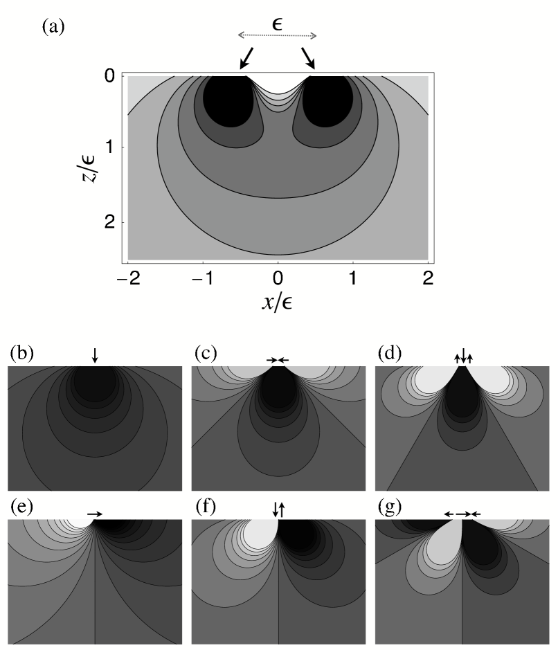
Figure 2: (a) Contour plot of pressure for two point forces of equal magnitude located at $\pm\epsilon/2$ and oriented at $\pm\pi/6$ from the surface normal. Distances are in units of $\epsilon$. The response is two-peaked for shallow depths, transitioning to the circular contours of $\sigma_{rr}$ for a single normal force at the origin. Monopole (b,e), dipole (c,f), and quadrupole (d,g) boundary forcings, along with contours of the corresponding pressures.

At distances larger than the separation between the points of application of the force, the stress field in Fig. 2a can be closely approximated by a multipole expansion. In a granular material, the local arrangement of grains in regions where strains are large will induce deviations from the continuum theory, and in the Boussinesq geometry the far field effects of these deviations can be approximated by placing a series of multipolar forcing terms at the origin. Thus, although the physical force applied by Geng et al., for example, was a single, sharply localized, normal force, we include in our continuum theory parameters specifying dipole, quadrupole, and perhaps higher order multipole forcing strengths to account for the effect of microstructure. If the applied force is spread over enough grains that the continuum solution predicts only small strains everywhere, then the multipole contributions can be explicitly computed within the continuum theory. If, on the other hand, the force is applied to a single grain and represented as a delta-function in the continuum theory, the theory will predict large strains near the origin and microstructure effects must be taken into account either phenomenologically, as we do here, or through a more detailed model of the microstructure in the vicinity of the applied force. We conjecture that the size of this region near the origin scales with the “isostaticity length scale” discussed in Refs. Wyart et al. (2005) and Ellenbroek et al. (2006).

The first several multipole forces and corresponding pressure profiles, are depicted in Fig. 2b-g. A multipole force with stresses that decay as $1/r^{n}$ can be constructed from $n$ evenly spaced compressive or shearing boundary forces having alternating directions and magnitudes in proportion to the $n^{\mathrm{th}}$ row of Pascal’s Triangle. The integral $\int_{-\infty}^{\infty}dx\,x^{n-1}{\bm{f}}(x)$ is the lowest order nonvanishing moment of the boundary force distribution ${\bm{f}}(x)$.

The form of the far-field stress response to multipole forcing in linear elasticity can be developed by considering the Airy stress function $\chi$ such that $\sigma_{rr}=\partial_{r}\chi/r+\partial_{\phi\phi}\chi/r^{2}$, $\sigma_{r\phi}=\sigma_{\phi r}=-\partial_{r}(\partial_{\phi}\chi/r)$, and $\sigma_{\phi\phi}=\partial_{rr}\chi$. The Airy stress function is biharmonic:

$$\bigtriangleup\bigtriangleup\chi=0.$$ (7)

Assuming $\chi$ has the form

$$\chi(r,\phi)=r^{2}\sum_{n=1}^{\infty}\frac{1}{r^{n}}\chi^{(n)}(\phi)$$ (8)

and solving for $\chi^{(n)}$ yields a series of corresponding tensors ${\bm{\sigma}}^{(n)}$. (It is convenient to restrict ourselves to transversely symmetric multipole terms, such as those in Fig. 2b-d, so that there is only one corresponding stress tensor for each value of $n$.) ${\bm{\sigma}}^{(1)}$ corresponds to the monopole of Eq. (1). For each ${\bm{\sigma}}^{(n)}$, $\sigma^{(n)}_{\phi\phi}$ and $\sigma^{(n)}_{r\phi}$ must vanish on the surface except at the origin. For the surface $C$ in Fig. 1 we generalize the monopole normalization to arbitrary $n$:

$$\int_{-\frac{\pi}{2}}^{-\frac{\pi}{2}}rd\phi\,(r\sin{\phi})^{n-1}\left(\hat{p}\cdot{\bm{\sigma}}^{(n)}\cdot\hat{r}\right) = 0$$

$$\int_{-\frac{\pi}{2}}^{-\frac{\pi}{2}}rd\phi\,(r\sin{\phi})^{n-1}\left(\hat{q}\cdot{\bm{\sigma}}^{(n)}\cdot\hat{r}\right) = ka^{n},$$ (9)

where $\hat{p}=\hat{x}$ ($\hat{z}$) and $\hat{q}=\hat{z}$ ($\hat{x}$) for odd (even) powers of $n$. $k$ and $a$ carry the units of stress and length, respectively, the applied force is $f=ka$. Subject to this normalization, the dipole stress tensor ${\bm{\sigma}}^{(2)}$ is

$$\sigma^{(2)}_{rr} = \frac{8ka^{2}}{\pi r^{2}}\cos{2\phi}$$

$$\sigma^{(2)}_{r\phi} = \frac{4ka^{2}}{\pi r^{2}}\sin{2\phi}$$

$$\sigma^{(2)}_{\phi\phi} = 0,$$ (10)

and the quadrupole stress tensor ${\bm{\sigma}}^{(3)}$ is

$$\sigma^{(3)}_{rr} = -\frac{5ka^{3}}{\pi r^{3}}\cos{3\phi}-\frac{3ka^{3}}{\pi r^{3}}\cos{\phi}$$

$$\sigma^{(3)}_{r\phi} = -\frac{3ka^{3}}{\pi r^{3}}\sin{3\phi}-\frac{3ka^{3}}{\pi r^{3}}\sin{\phi}$$

$$\sigma^{(3)}_{\phi\phi} = \hphantom{-}\frac{ka^{3}}{\pi r^{3}}\cos{3\phi}+\frac{3ka^{3}}{\pi r^{3}}\cos{\phi}.$$ (11)

Contours of the associated pressures $p^{(n)}=(1/2)\mathrm{Tr}\,{\bm{\sigma}}^{(n)}$ and sample boundary forces which produce them are shown in Fig. 2b-d.

The higher order multipole terms decay more quickly than the monopole term, so at asymptotically large depth in a material in which both monopole and higher order terms are present, the response is indistinguishable from the Boussinesq solution. Closer to the point of application, the induced multipole terms contribute more complex structure to the response. The distance over which this structure is observable depends on the material properties through the elastic coefficients and increases with the strength of the applied force $f$.

III Model free energies

Here we develop expressions for the elastic free energy of several model systems having hexagonal symmetry. These will be needed to construct constitutive relations relating stress and strain.

III.1 Symmetry considerations

To linear order the elastic energy is quadratic in the strain components:

$$A=\frac{1}{2}\lambda_{ijkl}\,\eta_{ij}\,\eta_{kl}.$$ (12)

$\lambda$ is a fourth order tensor of rank two, and its components are the elastic coefficients of the material. For an isotropic material the free energy must be invariant for rotations of $\eta$ through arbitrary angle. Therefore $A$ can depend only on scalar functions of the strain tensor components. In two dimensions, the strain tensor has two eigenvalues or principal invariants. All other scalar invariants, including the independent invariants $I_{1}=\mathrm{Tr}\,{\bm{\eta}}=\eta_{ii}$ and $I_{2}=\mathrm{Tr}\,{\bm{\eta}}^{2}=(\eta_{ij})^{2}$ (summation implied), can be expressed in terms of the principal invariants Spencer (1980) or, equivalently, in terms of $I_{1}$ and $I_{2}$. The free energy of an isotropic linear elastic material can be expressed in terms of combinations of $I_{1}$ and $I_{2}$ that are quadratic in the strain components.

$$A=\frac{1}{2}\lambda I_{1}^{2}+\mu I_{2}$$ (13)

where $\lambda$ and $\mu$ are the Lamé coefficients. The reasoning generalizes to higher orders. At each order, there will be as many elastic coefficients as there are independent combinations of $I_{1}$ and $I_{2}$. To quartic order in the strains, we have

$$A = \hphantom{+\quad}\biggl{(}\frac{1}{2}\lambda I_{1}^{2}+\mu I_{2}\biggr{)}$$ (14)

$$+\quad\biggl{(}\omega_{1}I_{1}^{3}+\omega_{2}I_{1}I_{2}\biggr{)}$$

$$+\quad\biggl{(}\Omega_{1}I_{1}^{4}+\Omega_{2}I_{2}^{2}+\Omega_{3}I_{1}^{2}I_{2}\biggr{)}.$$

We refer to the $\omega$’s and the $\Omega$’s as third and fourth order elastic coefficients, respectively.

To construct the free energy of a hexagonal material, it is useful to consider a change of coordinates

$$\xi = x+iz$$

$$\zeta = x-iz,$$ (15)

as suggested in Ref. Landau and Lifshitz (1997). For a rotation of $\pi/3$ about $(\hat{z}\times\hat{x})$ these coordinates transform as $\xi\rightarrow\xi e^{\pi i/3}$ and $\zeta\rightarrow\zeta e^{-\pi i/3}$. The free energy of an elastic material must be invariant under such a rotation, which implies that a component of the tensor $\lambda$ can be nonzero if and only if it too is invariant. For example, the quadratic coefficient $\lambda_{\xi\xi\zeta\zeta}$ is nonzero because, under rotation by $\pi/3$, $\lambda_{\xi\xi\zeta\zeta}\rightarrow e^{\pi i/3}e^{\pi i/3}e^{-\pi i/3}e^{-\pi i/3}\lambda_{\xi\xi\zeta\zeta}=\lambda_{\xi\xi\zeta\zeta}$. The only other independent nonzero quadratic coefficient is $\lambda_{\xi\zeta\xi\zeta}$. Cubic and higher order coefficients, which are labeled by six or more indices, can also be invariant by having six like indices, as in $\lambda_{\xi\xi\xi\xi\xi\xi}$. There are three independent coefficients at cubic order and four at quartic order.

The general form of the free energy of a hexagonal material is, to quartic order,

$$A = \hphantom{+\quad}\frac{1}{2!}\biggl{(}2\lambda_{1}\eta_{\xi\xi}\eta_{\zeta\zeta}+4\lambda_{2}\eta_{\xi\zeta}^{2}\biggr{)}$$ (16)

$$+\quad\frac{1}{3!}\biggl{(}\Lambda_{1}(\eta_{\xi\xi}^{3}+\eta_{\zeta\zeta}^{3})+12\Lambda_{2}\eta_{\xi\xi}\eta_{\xi\zeta}\eta_{\zeta\zeta}+8\Lambda_{3}\eta_{\xi\zeta}^{3}\biggr{)}$$

$$+\quad\frac{1}{4!}\biggl{(}6L_{1}\eta_{\xi\xi}^{2}\eta_{\zeta\zeta}^{2}+48L_{2}\eta_{\xi\xi}\eta_{\zeta\zeta}\eta_{\xi\zeta}^{2}\biggr{.}$$

$$\quad\quad\quad\quad\biggl{.}+16L_{3}\eta_{\xi\zeta}^{4}+8L_{4}(\eta_{\xi\xi}^{3}\eta_{\xi\zeta}+\eta_{\zeta\zeta}^{3}\eta_{\xi\zeta})\biggr{)}$$

where $\eta_{\xi\xi}=\eta_{xx}-\eta_{zz}+2i\eta_{xz}$, $\eta_{\zeta\zeta}=\eta_{xx}-\eta_{zz}-2i\eta_{xz}$, and $\eta_{\xi\zeta}=\eta_{xx}+\eta_{zz}$.

For simplicity, we have assumed that terms involving gradients of the strains are negligible Suiker et al. (2001); Walsh and Tordesillas (2004).

III.2 Hexagonal ball-and-spring network

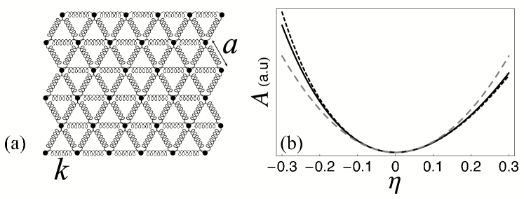
Figure 3: (a) A ball-and-spring network with hexagonal symmetry and springs oriented horizontally. Even for a linear force law, the free energy has terms of cubic and higher order in the strains when the equilibrium length of the springs is nonzero. (b) Free energy as a function of strain for a unit cell of the ball-and-spring network in (a). (solid black) Vertical uniaxial compression: $\eta=\eta_{zz}$ with $\eta_{yy}=0$. (dashed black) $\eta=\eta_{xx}$ with Horizontal uniaxial compression: $\eta_{zz}=0$. (dashed gray) Linear elastic approximation for both cases. $\eta<0$ corresponds to compression.

We now construct the free energy for several specific hexagonal materials, taking the point-mass-and-spring network of Fig. 3a as a starting point. The elastic coefficients are determined by calculating the free energy under a homogeneous strain and comparing to Eq. (16). The springs are taken to have an equilibrium length $\ell$ and to obey Hooke’s law: for a spring with one end at ${\bf x}_{1}$ and the other at ${\bf x}_{2}$ the force is

$$f=-k\left(\sqrt{({\bf x}_{2}-{\bf x}_{1})\cdot({\bf x}_{2}-{\bf x}_{1})}-\ell\right),$$ (17)

where $k$ is the spring constant. We take the springs to be at their equilibrium lengths in the undeformed system: $\ell=a$, the lattice constant.

Consider the homogeneous strain

$$\eta=\left(\begin{array}[]{cc}\eta_{xx}&0\\ 0&\eta_{zz}\end{array}\right)$$ (18)

which stretches the coordinates to $x=\sqrt{1+2\eta_{xx}}\,X$ and $z=\sqrt{1+2\eta_{zz}}\,Z$. The free energy per unit (undeformed) volume of a hexagonal ball-and-spring network with one third of the springs oriented along the $\hat{x}$ direction under this stretch is

$$\frac{4}{\sqrt{3}k}A = \hphantom{+\quad}\biggl{(}\frac{3}{2}\eta_{xx}^{2}+\frac{3}{2}\eta_{zz}^{2}+\eta_{xx}\eta_{zz}\biggr{)}$$ (19)

$$-\quad\biggl{(}+\frac{9}{8}\eta_{xx}^{3}+\frac{11}{8}\eta_{zz}^{3}+\frac{9}{8}\eta_{xx}^{2}\eta_{zz}+\frac{3}{8}\eta_{xx}\eta_{zz}^{2}\biggr{)}$$

$$+\quad\biggl{(}\frac{135}{128}\eta_{xx}^{4}+\frac{215}{128}\eta_{zz}^{4}+\frac{45}{64}\eta_{xx}^{2}\eta_{zz}^{2}\biggr{.}$$

$$\hphantom{\biggl{(}\quad\quad\quad\quad\quad}\biggl{.}+\frac{45}{32}\eta_{xx}^{3}\eta_{zz}+\frac{5}{32}\eta_{xx}\eta_{zz}^{3}\biggr{)}.$$

The presence of cubic and higher order terms in the free energy is due to the nonzero spring equilibrium length. The free energy for a constrained axial compression/extension in the $\hat{x}$ and $\hat{z}$ directions is plotted in Fig. 3. The corrections to the quadratic expression stiffen the system under compression and soften it slightly under small extensions.

Comparing Eqs. (16) and (19) and equating like coefficients of $\eta_{xx}$ and $\eta_{zz}$ we find

$$\begin{array}[]{ll}\vspace{0.1in}\lambda_{1}=\lambda_{2}=\frac{\sqrt{3}}{8}k\\ \vspace{0.1in}\Lambda_{1}=-\Lambda_{2}=-\Lambda_{3}=\frac{3\sqrt{3}}{32}k\\ L_{1}=L_{2}=L_{3}=-L_{4}=\frac{15\sqrt{3}}{128}k\end{array}$$ (20)

A similar calculation for a material in which one third of the springs are oriented vertically, corresponding to a reference configuration rotated by $90^{\circ}$ from the one shown in Fig. 3, yields

$$\begin{array}[]{ll}\vspace{0.1in}\lambda_{1}=\lambda_{2}=\frac{\sqrt{3}}{8}k\\ \vspace{0.1in}-\Lambda_{1}=-\Lambda_{2}=-\Lambda_{3}=\frac{3\sqrt{3}}{32}k\\ L_{1}=L_{2}=L_{3}=L_{4}=\frac{15\sqrt{3}}{128}k\end{array}$$ (21)

III.2.1 The $\alpha$-material

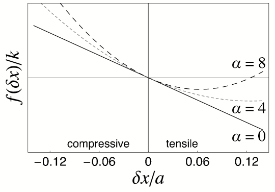
Figure 4: The force law of Eq. (22) for $k=1$ and $\alpha=0\ldots 8$.

Goldenberg and Goldhirsch Goldenberg and Goldhirsch (2002, 2004, 2005) find two-peaked stress response in numerical simulations of a hexagonal lattice of springs when the springs are allowed to break under tensile loading. Contact-breaking explicitly breaks our assumption of local hexagonal anisotropy in any particular sample. In the context of an ensemble average, however, the material description retains hexagonal symmetry and the effects of contact breaking are captured phenomenologically by considering material made of springs with a force law that softens under extension.

$$f = -k\left(\sqrt{({\bf x}_{2}-{\bf x}_{1})\cdot({\bf x}_{2}-{\bf x}_{1})}-a\right)$$ (22)

$$\quad\quad+k\frac{\alpha}{a}\left(\sqrt{({\bf x}_{2}-{\bf x}_{1})\cdot({\bf x}_{2}-{\bf x}_{1})}-a\right)^{2}.$$

For $\alpha>0$ the springs soften under tension and stiffen under compression, as shown in Fig. 4. In the horizontal orientation the elastic constants from Eq. (20) are shifted according to

$$\begin{array}[]{ll}\vspace{0.1in}\lambda_{1}=\lambda_{2}=\frac{\sqrt{3}}{8}k\\ \vspace{0.1in}\Lambda_{1}=-\Lambda_{2}=-\Lambda_{3}=\frac{3\sqrt{3}}{32}k-\frac{\alpha}{a}\frac{3\sqrt{3}}{32}k\\ L_{1}=L_{2}=L_{3}=-L_{4}=\frac{15\sqrt{3}}{128}k-\frac{\alpha}{a}\frac{9\sqrt{3}}{64}k\end{array}$$ (23)

III.2.2 The $\beta$-material

In the spirit of phenomenological modeling, all of the elastic constants consistent with hexagonal symmetry should be considered to be parameters to be determined by experiment. To probe the importance of hexagonal anisotropy, we consider a model in which all elastic constants but one are fixed and define a parameter $\beta$ corresponding to the strength of the anisotropy. Note that the elastic constants for the two orientations of the hexagonal ball-and-spring network considered above can be rewritten as

$$\begin{array}[]{ll}\vspace{0.1in}\lambda_{1}=\lambda_{2}=\frac{\sqrt{3}}{8}k&\\ \vspace{0.1in}\Lambda_{2}=\Lambda_{3}=-\frac{3\sqrt{3}}{32}k&\quad\Lambda_{1}=\beta\frac{3\sqrt{3}}{32}k\\ L_{1}=L_{2}=L_{3}=\frac{15\sqrt{3}}{128}k&\quad L_{4}=-\beta\frac{15\sqrt{3}}{128}k.\end{array}$$ (24)

The case $\beta=1$ gives the network with horizontal springs; $\beta=-1$ gives the network with vertical springs; and $\beta=0$ gives an isotropic system. Linear response for elastic materials with other ansisotropies is treated in Ref. Otto et al. (2003).

IV Method

We wish to obtain corrections to the linear elastic result for a material with hexagonal symmetry. For later convenience we write $f=Q_{m}ka$, where $Q_{m}$ is dimensionless, $k$ has units of a spring constant, and $a$ is a lattice constant with units of length. We expand the stress in successive inverse powers of the radial coordinate, and refer to the terms in the expansion as the dipole correction, quadrupole correction, and so forth. For simplicity and clarity, we present here the calculation corresponding to the free energy of Eq. (16) with coefficients given in Eq. (20) in detail. General equations for arbitrary elastic coefficients are exceedingly long and unilluminating.

We solve for the the displacements $u_{R}(R,\Phi)$ and $u_{\Phi}(R,\Phi)$, from which the stress tensor can be reconstructed. Capitalized coordinates are used as we are now careful to distinguish between the deformed and undeformed states. After the deformation, the point ${\bf X}$ is at ${\bf x}={\bf X}+u_{R}(R,\Phi))\hat{R}+u_{\Phi}(R,\Phi)\hat{\Phi}$. To linear order and for the ball-and-spring network described in Eq. (20) the displacements are

$$u_{R}^{(0)}(R,\Phi) = \frac{\sqrt{3}Q_{m}a}{\pi}\left(\cos{\Phi}\ln{\left(R/R_{0}\right)}+\frac{1}{3}\Phi\sin{\Phi}\right);$$

$$u_{\Phi}^{(0)}(R,\Phi) = \frac{\sqrt{3}Q_{m}a}{\pi}\left(\vphantom{\frac{1}{3}}-\sin{\Phi}\ln{\left(R/R_{0}\right)}\right.$$ (25)

$$\hphantom{\frac{\sqrt{3}Q_{m}a}{\pi}\biggl{(}\,}\left.-\frac{2}{3}\sin{\Phi}+\frac{1}{3}\Phi\cos{\Phi}\right).$$

The parameter $R_{0}$ requires comment. Because the material is semi-infinite in extent, it is free to undergo an arbitrary rigid-body translation in the $\hat{Z}$-direction under the influence of a normal boundary force. Thus the point along the $Z$-axis at which the deformation ${\bf u}$ is zero may be chosen arbitrarily. $R_{0}$ parameterizes this variation. Note that the nominal stress, which in the linear theory is equivalent to ${\bm{\sigma}}$ in Eq. (1), is independent of $R_{0}$.

To find the dipole correction, we take $u_{R}=u_{R}^{(0)}+u_{R}^{(1)}$ and $u_{\Phi}=u_{\Phi}^{(0)}+u_{\Phi}^{(1)}$ and assume a correction of the form

$$u_{R}^{(1)}(R,\Phi) = a^{2}\frac{v_{0}(\Phi)}{R}+a^{2}\frac{v_{1}(\Phi)}{R}\ln{\left(R/R_{0}\right)}$$

$$u_{\Phi}^{(1)}(R,\Phi) = a^{2}\frac{w_{0}(\Phi)}{R}+a^{2}\frac{w_{1}(\Phi)}{R}\ln{\left(R/R_{0}\right)}.$$ (26)

The deformation gradient ${\bf F}$ in polar coordinates is

$${\bf F}=\left(\begin{array}[]{cc}1+\partial_{R}u_{R}&\left(\partial_{\Phi}u_{R}-u_{\Phi}\right)/R\\ \partial_{R}u_{\Phi}&1+\left(\partial_{\Phi}u_{\Phi}+u_{R}\right)/R\end{array}\right).$$ (27)

Through Eqs. 3 and 6 the nominal stress can be written entirely in terms of the displacements, and through them in terms of the four unknown functions, $v_{0}$, $v_{1}$, $w_{0}$, and $w_{1}$.

Substituting the linear Boussinesq solution of Eq. 25 in Eq. 27, evaluating Eq. (4), and requiring the coefficient of $1/R^{3}$ to vanish yields conditions on the $v$’s and $w$’s. (Terms of smaller order in $1/R$ vanish identically.) We find

$$\!\!\!\!\!\!11-13\cos{2\Phi}-3\cos{4\Phi}-9\cos{6\Phi}-6\cos{8\Phi}$$

$$\quad=\frac{9}{2}v_{0}^{\prime\prime}-27v_{1}-27w_{0}^{\prime}+9w_{1}^{\prime}$$

$$\quad\hphantom{=}+\left(\frac{9}{2}v_{1}^{\prime\prime}-27w_{1}^{\prime}\right)\ln{\left(R/R_{0}\right)};$$

$$\!\!\!\!\!\!-5\sin{2\Phi}+\sin{4\Phi}+3\sin{6\Phi}+2\sin{8\Phi}$$

$$\quad=3v_{0}^{\prime}+3v_{1}^{\prime}+\frac{9}{2}w_{0}^{\prime\prime}-3w_{1}$$

$$\quad\hphantom{=}+\left(3v_{1}^{\prime}+\frac{9}{2}w_{1}^{\prime\prime}\right)\ln{\left(R/R_{0}\right)}.$$ (28)

For the moment, we neglect terms of higher order in $1/R$. The source terms on the left-hand side in Eq. (28) are generated by the linear solution. Requiring coefficients of $\ln R$ to vanish independently gives four second-order ordinary differential equations for the four unknown functions.

The conditions that normal and shear forces vanish everywhere on the deformed boundary except at the point of application of the external force can be written

$$S_{\Phi R}(R\neq 0,\Phi=\pm\pi/2) = 0$$

$$S_{\Phi\Phi}(R\neq 0,\Phi=\pm\pi/2) = 0.$$ (29)

Both the $S_{\Phi R}$ and $S_{\Phi\Phi}$ components of stress have terms proportional to $\ln{R}$. When we require these terms to vanish independently of all other terms, Eq. (29) represents eight constraints. The nominal stress must also satisfy force-transmission conditions

$$\int_{C}\,\hat{x}\cdot{\bf S}^{T}\cdot\hat{n}\,dC = 0$$

$$\int_{C}\,\hat{z}\cdot{\bf S}^{T}\cdot\hat{n}\,dC = f,$$ (30)

where $C$ is any surface enclosing the origin (see e.g. Fig. 1) and $\hat{n}$ is the unit normal to $C$. Eq. (30) is satisfied by the linear elastic solution, and all solutions to Eq. (28) subject to Eq. (29) contribute zero under the integration, so this provides no additional constraint on the system.

The eight constraints of Eq. (29) fix only seven of the eight integration constants. The eighth integration constant, which we label $Q_{d}$, multiplies terms identical to those contributed in linear elasticity by a horizontally oriented dipole forcing such as that depicted in Fig. 2c and given in Eq. (10). $Q_{d}$ is fixed by demanding that a variation of the parameter $R_{0}$ produce only a rigid body translation of the material. The integration constants determined in this way produce a nominal stress ${\bf S}$ independent of $R_{0}$, as must be the case.

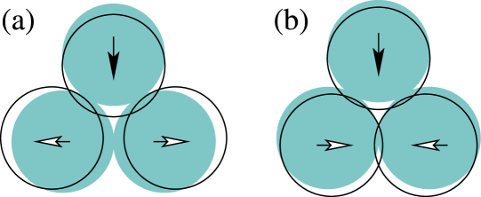
Figure 5: Two imagined scenarios in which a point force induces a dipole. Regions of overlap indicate a compressive contact. (a) The disks in the second layer slide outward, e.g. for low friction. (b) Alternatively the disks might roll inward, towards the line of force, e.g. due to greater friction between grains. This would select a dipole term in the stress response with opposite sign from the case depicted in (a). Thus, the details of the near field response depend on the mechanics of the discrete system.

The solution of Eq. 28 consistent with Eq. (29) is

$$v_{0}(\Phi) = \left(\frac{Q_{m}^{2}}{\pi^{2}}\right)\left[\frac{5}{6}+\frac{7}{3}\cos{2\Phi}\right.$$

$$\,\,\hphantom{\left(\frac{Q_{m}^{2}}{\pi^{2}}\right)}+\frac{1}{4}\cos{4\Phi}+\frac{1}{4}\cos{6\Phi}$$

$$\,\,\hphantom{\left(\frac{Q_{m}^{2}}{\pi^{2}}\right)}\left.+\frac{1}{12}\cos{8\Phi}+\frac{11}{6}\Phi\sin{2\Phi}\right]$$

$$-\left(\frac{4\pi Q_{d}}{\sqrt{3}}\right)\cos{2\Phi};$$

$$v_{1}(\Phi) = \left(\frac{3Q_{m}^{2}}{2\pi^{2}}\right)\cos{2\Phi}\ln{\left(R/R_{0}\right)};$$

$$w_{0}(\Phi) = -\left(\frac{Q_{m}^{2}}{\pi^{2}}\right)\left[\frac{11}{9}\Phi+\frac{2}{3}\sin{2\Phi}\right.$$

$$\,\,\hphantom{-\left(\frac{Q_{m}^{2}}{\pi^{2}}\right)}+\frac{1}{12}\sin{4\Phi}+\frac{1}{12}\sin{6\Phi}$$

$$\,\,\hphantom{-\left(\frac{Q_{m}^{2}}{\pi^{2}}\right)}\left.+\frac{1}{36}\sin{8\Phi}-\frac{11}{18}\Phi\cos{2\Phi}\right]$$

$$+\left(\frac{4\pi Q_{d}}{3\sqrt{3}}\right)\sin{2\Phi}$$

$$w_{1}(\Phi) = -\left(\frac{Q_{m}^{2}}{2\pi^{2}}\right)\sin{2\Phi}\ln{\left(R/R_{0}\right)}.$$ (31)

For the choice $R_{0}=a$, we find the induced dipole coefficient $Q_{d}=0$, and for the sequel we fix $R_{0}$ to have this value. The same choice of $R_{0}$ also yields the induced quadrupole coefficient $Q_{q}=0$ below. As discussed above, rather than set them to zero, we leave these terms in the displacements, and correspondingly the stresses, as free parameters to account for the influence of microstructure on the response. They are weighted so that $Q_{d}=1$ and $Q_{q}=1$ correspond to the stresses of Eqs. (10) and (11).

We repeat the process described above to develop quadrupole corrections to the stress response. The displacements are assumed to have the form $u_{R}(R,\Phi)=u_{R}^{(0)}(R,\Phi)+u_{R}^{(1)}(R,\Phi)+u_{R}^{(2)}(R,\Phi)$ and $u_{\Phi}(R,\Phi)=u_{\Phi}^{(0)}(R,\Phi)+u_{\Phi}^{(1)}(R,\Phi)+u_{\Phi}^{(2)}(R,\Phi)$ where the second order corrections have the form

$$u_{R}^{(2)}(R,\Phi) = \frac{V_{0}(\Phi)}{R^{2}}+\frac{V_{1}(\Phi)}{R^{2}}\ln{\left(R/R_{0}\right)}$$

$$+\frac{V_{2}(\Phi)}{R^{2}}\ln{\left(R/R_{0}\right)}^{2};$$

$$u_{\Phi}^{(2)}(R,\Phi) = \frac{W_{0}(\Phi)}{R^{2}}+\frac{W_{1}(\Phi)}{R^{2}}\ln{\left(R/R_{0}\right)}$$ (32)

$$+\frac{W_{2}(\Phi)}{R^{2}}\ln{\left(R/R_{0}\right)}^{2}.$$

The details of the calculation are omitted, as they are conceptually similar to the dipole calculation but involve much longer expressions. Defining $c_{n}\equiv\cos{n\Phi}$, $s_{n}\equiv\sin{n\Phi}$, and $L\equiv\ln{(R/R_{0})}$, the pressure is

$$p(r(R,\Phi),\phi(R,\Phi)) = \frac{Q_{m}ka}{\pi}\frac{c_{1}}{R}-\frac{4Q_{d}ka^{2}}{\pi}\frac{c_{2}}{R^{2}}-\frac{2Q_{q}ka^{3}}{\pi}\frac{c_{3}}{R^{3}}$$ (33)

$$+\frac{B_{2}}{R^{2}}\biggl{[}17-c_{2}-6c_{4}-9c_{6}-4c_{8}-22\Phi s_{2}-18Lc_{2}\biggr{]}$$

$$+\frac{B_{3}}{R^{3}}\biggl{[}-\frac{99}{2}c_{1}+\left(\frac{616277}{8820}-\frac{27}{7}\pi^{2}+\frac{41}{3}\Phi^{2}\right)c_{3}+\frac{205}{2}c_{5}+\frac{139}{3}c_{7}+25c_{9}\biggr{.}$$

$$\hphantom{\frac{B_{3}}{R^{3}}\biggl{[}}+\frac{63}{4}c_{11}+\frac{119}{10}c_{13}+\frac{10}{3}c_{15}-\Phi\left(66s_{1}+161s_{3}-66s_{5}-88s_{7}-\frac{110}{3}s_{9}\right)\biggr{.}$$

$$\hphantom{\frac{B_{3}}{R^{3}}\biggl{[}}+L\left(-48c_{1}-\frac{329}{3}c_{3}+36c_{7}+30c_{9}-42\Phi s_{3}\right)-27L^{2}c_{3}\biggr{]}$$

$$+\frac{B_{3}^{\prime}}{R^{3}}Q_{d}\biggl{[}8c_{1}-\frac{151}{14}c_{3}-6c_{7}-5c_{9}+7\Phi s_{3}+9Lc_{3}\biggr{]},$$

where $B_{2}=Q_{m}^{2}ka^{2}/12\sqrt{3}/\pi^{2}$, $B_{3}=Q_{m}^{3}ka^{3}/36\pi^{3}$, and $B_{3}^{\prime}=4Q_{m}^{3}ka^{3}/3\sqrt{3}\pi^{2}$.

We will find below that the $\beta$-material best describes the data of Ref. Geng et al. (2001). In this case the pressure of Eq. (33) gains a number of additional terms involving $\beta$. These terms are given in the Appendix.

V Results

Given the expressions derived above for the pressure, we perform numerical fits to the data from Geng et al. Geng et al. (2001). There are four fitting parameters for the ball-and-spring material: the monopole coefficient $Q_{m}$, the dipole coefficient $Q_{d}$, the quadrupole coefficient $Q_{q}$, and the spring constant $k$. We take the lattice constant to be the disk diameter: $a=0.8\,$cm. The three multipole coefficients have been defined to be dimensionless. We set $R_{0}=a$ so that $Q_{d}$ and $Q_{q}$ would be zero in a theory with no microstruture correction. In two dimensions the units of stress are the same as the units of the spring constant $k$. Thus $k$ sets the overall scale for the stress. For theoretical purposes, $k$ could be scaled to unity; in our fits it serves merely to match the units of stress in the experimental data.

We attempt to fit experimental measurements on pentagonal-grain packings by varying $Q_{m}$, $Q_{d}$ and $Q_{q}$ in the isotropic theory. To explain the experimental data on hexagonal disk packings, we attempt fits based on the ball-and-spring network, the $\alpha$-material, and the $\beta$-material.

We regard the response profiles presented in the following section, particularly Figs. 6 and 9, as a proof of principle: average response in experiments of the sort performed in Ref. Geng et al. (2001) is consistent with an elastic continuum approach when microstructure and material order are properly incorporated. The results we present are phenomonological in that we have obtained elastic coefficients and multipole strengths by fitting to data. We expect that the elastic coefficients we fit are material properties in the sense that they could be determined by experiment or simulation in another geometry (e.g. a uniform shear or compression), then used in our calculations for point response.

V.1 Fitting to pressure

The photoelastic measurements of Geng et al. associate a scalar quantity with each point in space. The measurement technique extracts no directional information, so the relevant theoretical prediction to compare to experiment is the local pressure $p=(1/2)\mathrm{Tr}\,{\bm{\sigma}}$ Geng (2003).

The data of Ref. Geng et al. (2001) are averaged over many experimental realizations; the average hydrostatic head is also subtracted. The hydrostatic contribution to the stress is largest at depth where, as seen below, the linear (monopole) response dominates. Therefore, although the elasticity theory is nonlinear and superposition does not strictly hold, we expect the incurred error from differencing to be small. We note also that our fits necessarily produce regions of small tensile stress near the surface. Removal of all tensile stresses from the solution would require treating the nonlinearity associated with contact breaking to all orders in the nonlinear elasticity theory. In the present context, such regions should be taken only as indicating that contacts are likely to break.

Fitting to the Cauchy pressure $p$, which is a natural function of the deformed coordinates ${\bf x}$, presents a difficulty. Namely, our caluclations yield a relation ${\bf x}={\bf X}+{\bf u}({\bf X})$ that is not invertible. Although in principle ${\bm{\sigma}}$ is known for all points in the deformed material, we can still only reference those points by their undeformed positions. That is, we have calculated $p({\bf x}({\bf X}))$. Thus for the purposes of fitting, we neglect the difference betwen ${\bf x}$ and ${\bf X}$. In the experiment, the forcing was restricted to strengths for which the strains were small; there were no large-scale rearrangements. This suggests that replacing the deformed coordinates with the undeformed coordinates will introduce only small errors. Of course, if the strains are small, it is reasonable to ask whether nonlinear elasticity is really needed or helpful. A discussion of this point is provided in Section VI below.

To facilitate comparison between various materials, we restrict our consideration to boundary forces $f=Q_{m}ka$ with $Q_{m}=1$. We have found that similar response profiles can be obtained for $0.25\leq Q_{m}\leq 2$, and all best-fit values for $Q_{m}$ lie in this range. The force $f=ka$ is that required to compress one Hookean spring through one lattice constant.

Rather than compare pressure directly to the data of Ref. Geng et al. (2001), we scale each data point by its depth $Z$ and fit to $Z\,P(X,Z)$ for two depths: $Z=2.7$ cm and 3.60 cm (recall that the grain diameter is 0.80 cm). Scaling by $Z$ compensates for the decay of the response with depth. For a reasonable fit, fitting to data at one or two shallow depths gives good agreement with all data at greater depth. Generally the fitting algorithm returns parameters such that agreement with experimental profiles at depths shallower than the shallowest fitting depth is poor. For the best model material, however, it is possible to achieve reasonable agreement with data at a depth of 2.25 cm.

V.2 Pentagonal particles

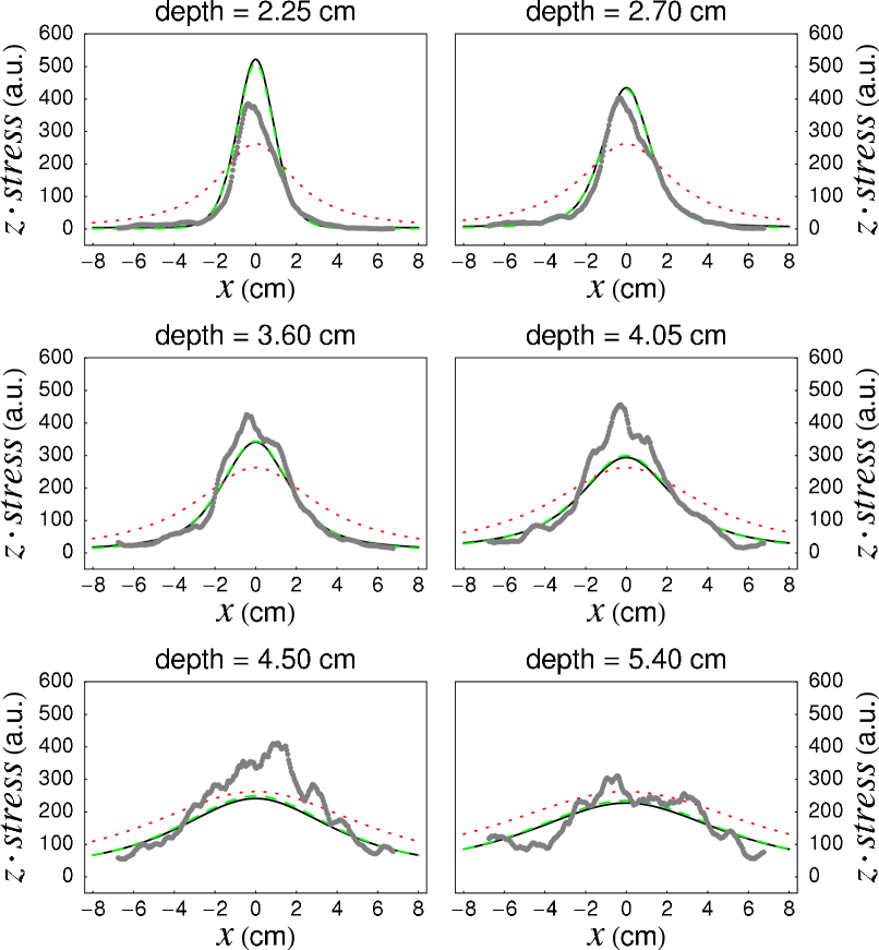
Figure 6: (color online) (black curves) A fit of Cauchy pressure for a spring-like isotropic ($\beta=0$) material with free energy expanded to quartic order in the strains. The fit parameters are $Q_{m}=1$, $Q_{d}=0.5$, $Q_{q}=-4.6$, and $k=702$ and were determined by fitting to response in a packing of pentagonal particles (gray points) of width $0.8\,$cm at depths $Z=2.7\,$cm and 3.60 cm. (dashed green curves) Linear elastic multipole response with $Q_{m}=1$, $Q_{d}=0.6$, $Q_{q}=-4.0$, and $k=700$, fit to the same data. (dotted red curves) Linear elastic monopole response with $Q_{m}=1$ and $k=1032$.

The nominal pressure of the spring-like isotropic ($\beta=0$) material for $Q_{m}=1$, $Q_{d}=0.5$, $Q_{q}=-4.6$, and $k=702$ is shown in Fig. 6. Parameters were determined by fitting to mean pentagonal particle response data. The result is a clear improvement over the fit to linear elastic pressure; the nonlinear calculation is able to capture the narrowing of the response as $Z\rightarrow 0$. At $Z=2.25\,$cm, shallower than the fitting data, the curve has an appropriate width but overshoots the peak. Note that there is little reason a priori to assume the elastic coefficients we have chosen are the appropriate ones to describe this material.

A multipole expansion

$$p=\frac{Q_{m}ka}{\pi R}\cos{\Phi}+\frac{4Q_{d}ka^{2}}{\pi R^{2}}\cos{2\Phi}-\frac{2Q_{q}ka^{3}}{\pi R^{3}}\cos{3\Phi}$$ (34)

with $Q_{m}=1$, $Q_{d}=0.6$, $Q_{q}=-4.0$, and $k=700$ is nearly indistinguishable from the full nonlinear expression with microstructure correction. This suggests that in the disordered packings the deviation from monopole-like linear elastic response is a consequence of microstructure, not effects captured by the nonlinear theory.

V.3 Hexagonal packings

V.3.1 Ball-and-spring fit

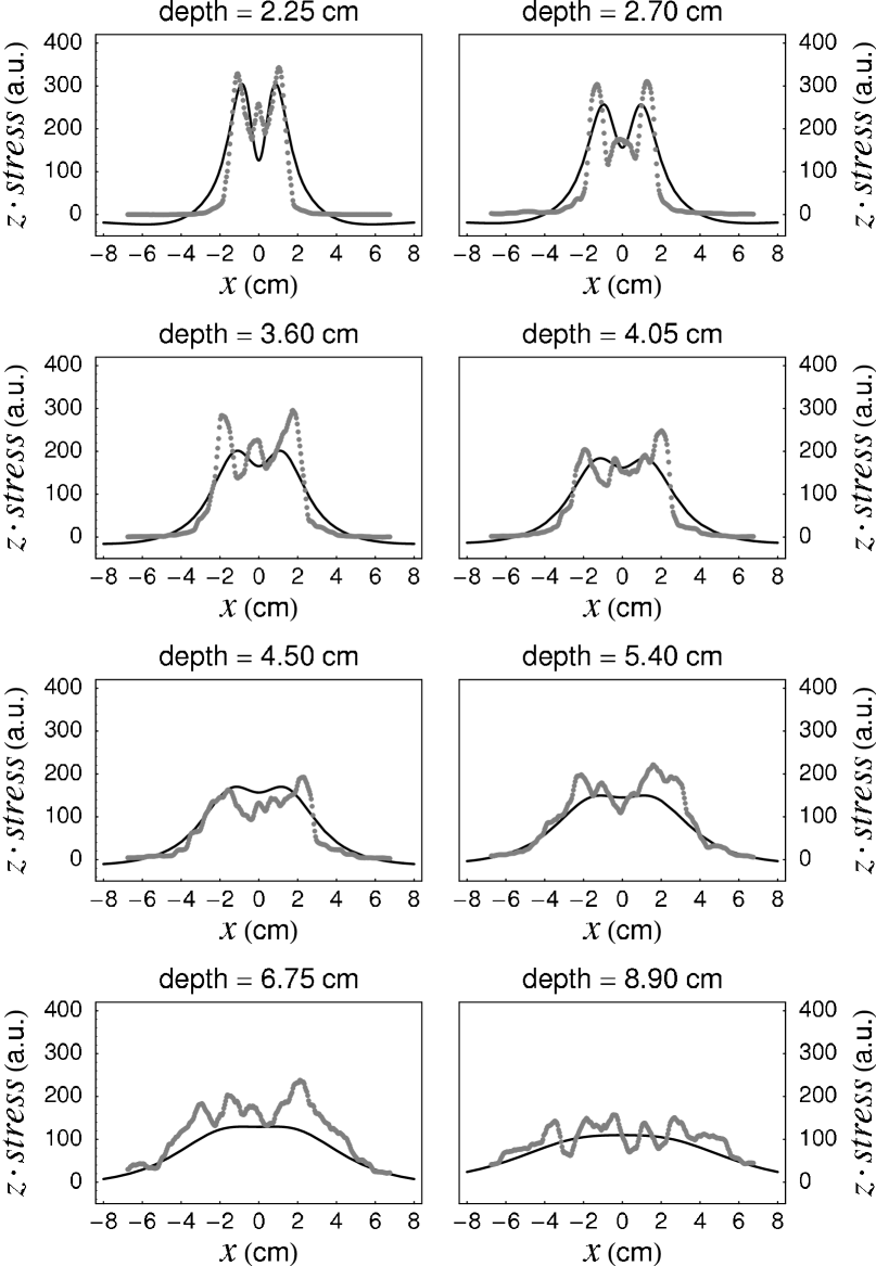
Figure 7: (black curves)A fit of Cauchy pressure for a ball-and-spring network including cubic and quartic corrections to the free energy. The fit parameters are $Q_{m}=1$, $Q_{d}=9.1$, $Q_{q}=32$, and $k=112$ and were determined by fitting to response in a monodisperse hexagonal packing of disks (gray points) of diameter $0.8\,$cm at depths $Z=2.7\,$cm and 3.60 cm.

The nominal pressure of the ball-and-spring network for $Q_{m}=1$, $Q_{d}=9.1$, $Q_{q}=36$ and $k=112$ is shown in Fig. 7. Parameters were determined by fitting to mean hexagonal packing response data. The pressure has two peaks at shallow depths; by $Z=5\,$cm it has crossed over to a single central peak. As expected, the elastic prediction improves with depth, as the monopole term, which is independent of all elastic coefficients, comes to dominate. For depths $z\lesssim 3\,$cm there are clear qualitative differences between the fit and the data. The two large peaks in the data are wider apart than the prediction and they fall off more sharply with horizontal distance from the center; moreover, the theoretical prediction fails to capture the small central peak in the data.

V.3.2 $\alpha$-material fit

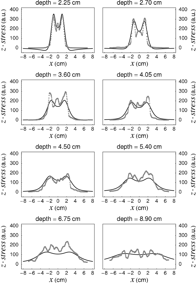
Figure 8: (black curves) A fit of Cauchy pressure for the $\alpha$-material including cubic and quartic corrections to the free energy. The fit parameters are $Q_{m}=1$, $Q_{d}=0.9$, $Q_{q}=-15$, $k=354$, and $\alpha=8.9$ and were determined by fitting to response in a monodisperse hexagonal packing of disks (gray points) of diameter $0.8\,$cm at depths $Z=2.7\,$cm and 3.60 cm.

The nominal pressure of the $\alpha$-material for $Q_{m}=1$, $Q_{d}=0.9$, $Q_{q}=-15.4$, $k=354$ and $\alpha=8.9$ is shown in Fig.8. The pressure response in the $\alpha$-material is a better fit than that for the ball-and-spring network, as it more closely recreates the two-peaked structure from $Z\approx 4\,$cm to 6 cm. It also drops off more sharply in the wings than the ball-and-spring response. The central peak, however, is still absent. Moreover, a value of $\alpha\approx 9$ is fairly large (see Fig. 4).

V.3.3 $\beta$-material fit

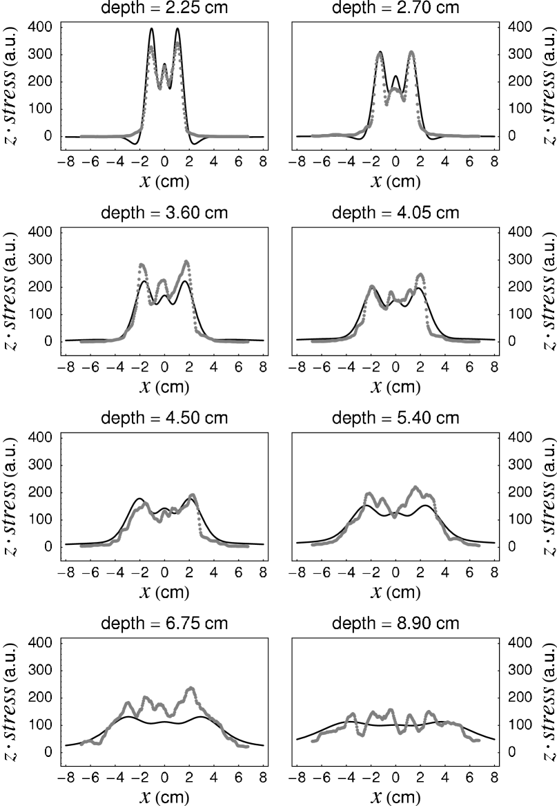
Figure 9: (black curves) A fit of Cauchy pressure for the $\beta$-material including cubic and quartic corrections to the free energy. The fit parameters are $Q_{m}=1$, $Q_{d}=0.6$, $Q_{q}=-2.0$, $k=353$, and $\beta=12.4$ and were determined by fitting to response in a monodisperse hexagonal packing of disks (gray points) of diameter $0.8\,$cm at depths $Z=2.7\,$cm and 3.60 cm.

The nominal pressure of the $\beta$-material for $Q_{m}=1$, $Q_{d}=0.6$, $Q_{q}=-2.0$, $k=353$ and $\beta=12.4$ is shown in Fig. 9. Parameters were determined by fitting to mean hexagonal response data. The $\beta$-material response does a better job of capturing the peaks than both the ball-and-spring material and $\alpha$-material response profiles. Like the $\alpha$-material, the shape of the response peaks of the $\beta$-material is narrower and more appropriately positioned than that of the ball-and-spring material. The $\beta$-material profiles do a better job capturing the small central peak, though the required $\beta$ value of $12.4$ represents a hexagonal anisotropy that is very strong compared to that of a simple ball-and-spring network.

Fig. 10 shows the $\beta$-material response without microstructure correction ($Q_{m}=1$, $\beta=10.8$, $k=509$) and the linear elastic response with induced multipole terms of Eq. (34) ($Q_{m}=1$, $Q_{d}=11.4$, $Q_{q}=42$, $k=116$). Neither agrees well with the data. It is necessary to include nonlinear as well as microstructure corrections to the linear elastic result to obtain good agreement with the mean hexagonal response data. This contrasts with the mean disordered response data, which can be described with a microstructure correction alone. We infer that nonlinear corrections are needed in the hexagonal system to capture the material anisotropy.

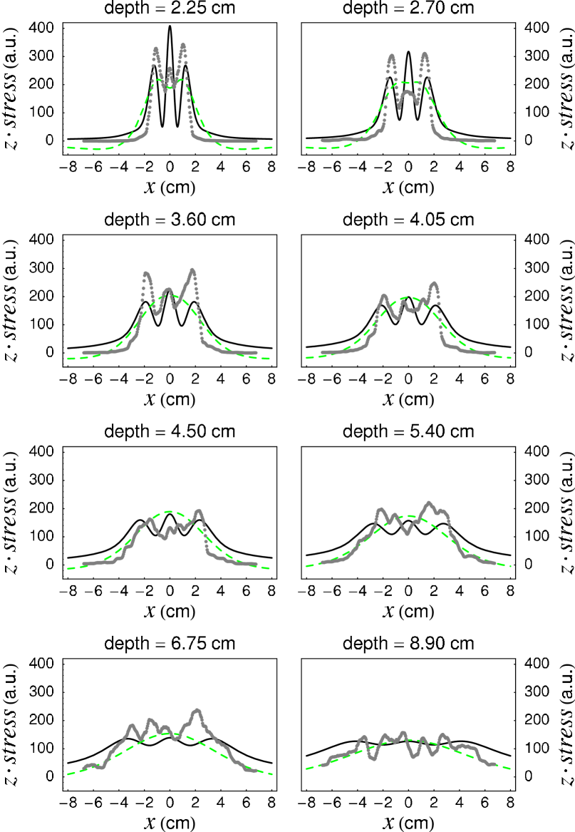
Figure 10: (color online) (black curves) A fit of Cauchy pressure for the $\beta$-material including cubic and quartic corrections to the free energy but without multipole corrections for microstructure ($Q_{d}=0=Q_{m}$). The fit parameters are $Q_{m}=1$, $k=509$, and $\beta=10.8$ and were determined by fitting to response in a monodisperse hexagonal packing of disks (gray points) of diameter $0.8\,$cm at depths $Z=2.7\,$cm and 3.60 cm. (dashed green curves) Linear elastic multipole response with $Q_{m}=1$, $Q_{d}=11.4$, $Q_{q}=43$, and $k=116$, fit to the same data.

V.4 Crossover to linear elasticity

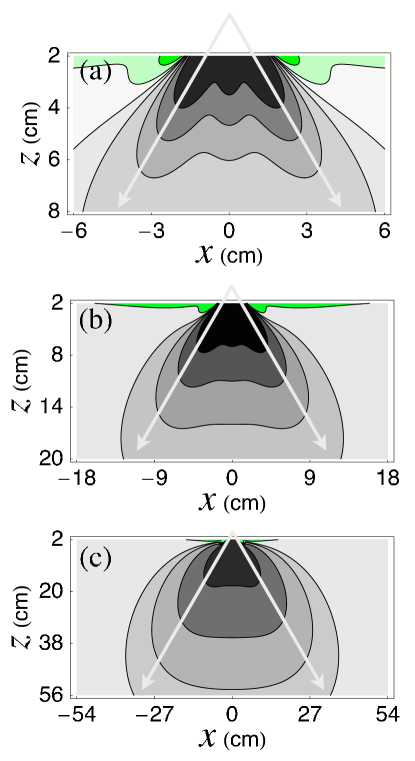
Figure 11: (color on-line) Pressure contours for the $\beta$-material with fit parameters identical to those in Fig. 9. At shallow depths the structure is three-peaked, the outer two seeming to propagate with depth. At greater depth the crossover to monopole response is evident. Regions of tensile stress near the surface are plotted in green.

For shallow depths the hexagonal anisotropy of the ordered disk packing is strongly reflected in the functional form of its stress response. The dipole and quadrupole corrections which shape the response in the near field fall off as $1/R^{2}$ and $1/R^{3}$, respectively, while the monopole response decays as $1/R$. Sufficiently deep within the material, the monopole term, which is identical to the linear elastic solution, will dominate. Fig. 11 shows contours of the nominal pressure for the $\beta$-material of Fig. 9 in the near and far fields. In the first $6\,$cm of depth the three peaks seen in the data are clearly visible. The contours of the pressure in linear elasticity are circles, and by a depth of $40\,$cm this form is largely recovered.

V.5 Physical pressure and strain

(a)
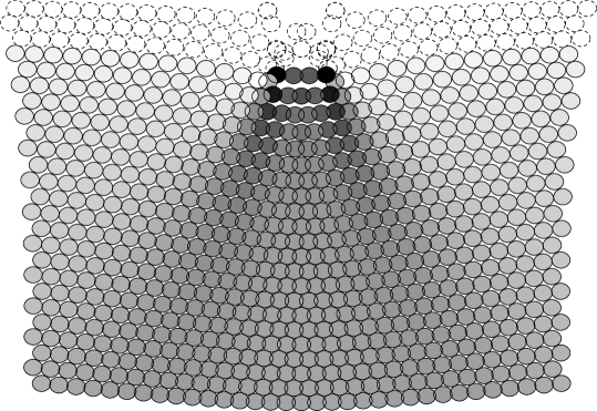
(b)

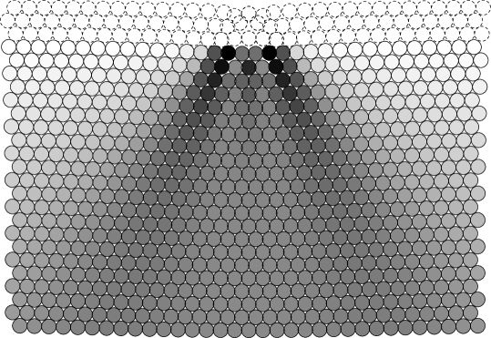
Figure 12: (a) The deformed $\beta$-material. The first three layers of the material are omitted. Disk $i$ with lattice position ${\bf X}_{i}$ in the undeformed material is shown here centered at ${\bf x}_{i}$. Each disk is shaded according to $R_{i}p_{i}$, the physical pressure scaled by the (undeformed) distance from the point force; values increase from blue through purple and orange to green. Pressures are calculated for the case for $Q_{m}=1$, $Q_{d}=0.6$, $Q_{q}=-2.0$, $k=353$ and $\beta=12.4$. Two-peaked structure is apparent, as well as arching in the upper layers. The strains are large. (b) The deformed $\beta$-material for $Q_{m}=1/4$, $Q_{d}=0.12$, $Q_{q}=-1.2$, $k=1415$ and $\beta=45.7$.

Having determined fit parameters, it is possible to visualize the physical or Cauchy pressure $p=(1/2)\mathrm{Tr}{\bm{\sigma}}({\bf x}({\bf X}))$ and strains in the material. In the undeformed material, each disk sits on a lattice site which we label by an index $i$. Under the deformation the disk at ${\bf X}_{i}$ moves to ${\bf x}_{i}={\bf X}_{i}+{\bf u}_{i}$. We draw a disk of radius $D=0.8\,$cm at ${\bf x}_{i}$ and shade it in proportion to $|{\bf X}_{i}|p_{i}({\bf x}_{i}({\bf X}_{i}))$. The first three layers of the packing, for which the displacements and pressure are clearly diverging near the applied force, are drawn but not shaded. Though we do not make any attempt to portray the deformations of the disks themselves, the overlap or separation between disks gives a good sense of the strain in the material, and the colormap indicates the local variation of pressure on the grain scale. The $\beta$-material fit for $Q_{m}=1$ is shown in Fig. 12. The two-peaked response structure is immediately apparent; the smaller third peak is more difficult to see, but present for the first few rows. There is dilatation near the surface. The disks directly below the applied force participate in the formation of arches, which is consistent with the appearance of two large peaks along the lines $\phi=\pm\pi/6$.

VI Strain magnitude

We have demonstrated that hexagonally anisotropic nonlinear elastic response can display stress profiles similar to those seen in ordered granular packings, which suggests that significant deviations from the classical Boussinesq response can extend to depths of tens of layers. However, from Fig. 12a it is also clear that the attendant strains are large, creating regions of strains in the first two dozen layers that are much larger than those observed in the systems studied by Geng et al. This is not entirely surprising for the choice $Q_{m}=1$. We note, however, that by fixing $Q_{m}=1/4$, as in Fig. 12b, we obtain a fit in which strains outside the first three layers are reasonably small. Differences from the response profiles in Fig. 9 are imperceptibly small; plotted on top of Fig. 9, the $Q_{m}=1/4$ and $Q_{m}=1$ curves would overlap. The microstructure corrections are still of order unity, the spring constant is four times larger (so that the imposed force $f$ is unchanged), and the hexagonal anisotropy is increased significantly: $\beta=45.7$. Thus in a our simplistic ball-and-spring-inspired material, the observed profiles can be attributed either to strong nonlinearity due to large strain magnitude or to strong hexagonal anisotropy.

The material constants of Eq. (24) were chosen as a minimal hexagonally anisotropic model, rather than derived from a microscopic model. We speculate that the enhancement of the nonlinearity and/or the hexagonal anisotropy over the values obtained naturally from simple ball-and-spring models may be due to the importance of a short length scale $\delta\ll D$ in the grain-grain interactions. Such a length scale may be the consequence of, e.g., nonlinear grain interactions (“soft shell” grains de Gennes (1999) or Hertzian force laws), or inhomogeneous elastic coefficients due to microscopic grain irregularities Goldenberg and Goldhirsch (2002); DiDonna and Lubensky (2005), in which case small strains may correspond to large deformations of contacts on the relevant scale $\delta$. Full consideration of such effects is beyond the scope of the present work.

Considering all the results presented above, we arrive at the following picture. The important distinctions between 2D disordered and hexagonal granular packings are the effects near the applied point force and the material symmetry. Although nonlinearity complicates calculations considerably, it enters only as a matter of necessity in incorporating material order: elasticity cannot distinguish isotropic and hexagonally anisotropic materials otherwise. The facts that 1) nonlinearities in the isotropic material provide no notable improvement over microstructure corrections alone (see Fig. 6), and 2) hexagonal materials admit reasonable response profiles for small strain and strong anisotropy (see Fig. 12b), underscore this point. A large $\beta$ value may be difficult to interpret in terms of a microscopic model, but this is not surprising given that it represents a combination of strong local nonlinearites and an ensemble average over microstructures that are known to lead to vastly different stress or force chain patterns.

VII Conclusion

Our results indicate that continuum elasticity theory can provide semi-quantitative explanations of nontrivial experimental results on granular materials. For isotropic (disordered) materials subject to a point force, it appears that nonlinearities are less important than multipoles induced at the surface where continuum theory breaks down. For hexagonal disk packings, however, the anisotropy associated with nonlinear terms in the elasticity theory is required. We have studied the nonlinear theory of response in a hexagonal lattice of point masses connected by springs and a phenomenological free energy with an adjustable parameter determining the strength of the hexagonal anisotropy. A similar treatment would be possible for systems with, e.g. , square or uniaxial symmetry, but the free energy would acquire additional terms at all orders. For a particular choice of elastic coefficients, the multiple peaks in the pressure profile at intermediate depths and the recovery of the familiar single peak of conventional (linear) elasticity theory at large depths are well described by the theory. To the extent that theoretical approaches based on properties of isostatic systems predict hyperbolic response profiles Blumenfeld (2004), our analysis indicates that the materials studied in Refs. Geng et al. (2001) and Geng et al. (2003) have average coordination numbers that place them in the elastic rather than isostatic regime.

Appendix A Pressure in the $\beta$-material

The expression of Eq. (33) gives the pressure in a horizontally oriented ball-and-spring network with elastic coefficients given by Eq. (16). The pressure in the $\beta$-material of Eq. (24) is given by adding an additional term $p_{\beta}(r(R,\Phi),\phi(R,\Phi))$ to the expression in Eq. (33), where $p_{\beta}$ is given by

$$p_{\beta}(r(R,\Phi),\phi(R,\Phi)) = \frac{B_{2}}{R^{2}}\beta\biggl{[}-6c_{4}-9c_{6}-4c_{8}\biggr{]}$$ (35)

$$+\frac{B_{3}}{R^{3}}\beta\biggl{[}\frac{28333}{420}c_{3}+\frac{205}{2}c_{5}+\frac{139}{3}c_{7}+\frac{35}{2}c_{9}\biggr{.}$$

$$\hphantom{\frac{B_{3}}{R^{3}}\beta\biggl{[}}+2\Phi\biggl{(}-62s_{3}+33s_{5}+44s_{7}+\frac{55}{3}s_{9}\biggr{)}\biggr{.}+L\biggl{(}-50c_{3}+36c_{7}+30c_{9}\biggr{)}\biggr{]}$$

$$+\frac{B_{3}}{R^{3}}\beta^{2}\biggl{[}9c_{1}-\frac{10418}{735}c_{3}+\frac{15}{2}c_{9}+\frac{63}{4}c_{11}\biggr{.}+\frac{119}{10}c_{13}+\frac{10}{3}c_{15}+36\Phi s_{3}+24Lc_{3}\biggr{]}$$

$$+\frac{B_{3}^{\prime}Q_{d}}{\sqrt{3}\pi R^{3}}\beta\biggl{[}\frac{5\sqrt{3}\pi}{14}c_{3}+\frac{28333\pi}{6720}c_{3}+\frac{205\pi}{32}c_{5}-6\sqrt{3}\pi c_{7}+\frac{139}{48}c_{7}-5\sqrt{3}\pi c_{9}+\frac{35}{32}c_{9}\biggr{.}$$

$$\hphantom{+\frac{B_{3}^{\prime}Q_{d}}{\sqrt{3}\pi R^{3}}\beta\biggl{[}}+\Phi\biggl{(}-\frac{31}{4}s_{3}+\frac{33}{8}s_{5}+\frac{11}{2}s_{7}-\frac{55}{24}s_{9}\biggr{)}+L\biggl{(}-\frac{25}{8}c_{3}+\frac{9}{4}c_{7}+\frac{15}{8}c_{9}\biggr{)}\biggr{]}$$

$$+\frac{B_{3}^{\prime}Q_{d}}{\sqrt{3}\pi R^{3}}\beta^{2}\biggl{[}\frac{9}{16}c_{1}-\frac{5209}{5880}c_{3}+\frac{15}{32}c_{9}+\frac{63}{64}c_{11}+\frac{119}{160}c_{13}+\frac{5}{24}c_{15}\biggr{.}+\frac{9}{4}\Phi s_{3}+\frac{3}{2}Lc_{3}\biggr{]}$$

References

- Geng et al. (2001) J. Geng, D. Howell, E. Longhi, R. P. Behringer, G. Reydellet, L. Vanel, E. Clément, and S. Luding, Phys. Rev. Lett. 87, 035506 (2001).
- Geng et al. (2003) J. Geng, G. Reydellet, E. Clément, and R. P. Behringer, Physica D 182, 274 (2003).
- Serero et al. (2001) D. Serero, G. Reydellet, P. Claudin, E. Clément, and D. Levine, Eur. Phys. J. E 6, 169 (2001).
- Reydellet and Clément (2001) G. Reydellet and E. Clément, Phys. Rev. Lett. 86, 3308 (2001).
- Mueggenburg et al. (2002) N. W. Mueggenburg, H. M. Jaeger, and S. R. Nagel, Phys. Rev. E 66, 031304 (2002).
- Spannuth et al. (2004) M. J. Spannuth, N. W. Mueggenburg, H. M. Jaeger, and S. R. Nagel, Granular Matter 6, 215 (2004).
- Head et al. (2001) D. Head, A. Tkachenko, and T. Witten, Eur. Phys. J. E 6, 99 (2001).