Realistic solution to the tunneling time problem

Abstract

There remains the old question of how long a quantum particle takes to tunnel through a potential barrier higher than its incident kinetic energy. In this article a solution of the question is proposed on the basis of a realistic explanation of quantum mechanics. The explanation implies that the tunneling particle has a certain chance to borrow enough energy from self-interference to high-jump over the barrier. The root-mean-square velocity and the effective tunneling time of an electron tunneling through a rectangular barrier are numerically calculated. No superluminal effect (Hartman effect) is found for the tunneling electron. Heisenberg’s energy-time uncertainty relation for the tunneling effect is verified by calculating an introduced coefficient representing uncertainty. The present author argues that phase time, dwell time and Bütticker-Landauer time are not appropriate expressions for the actual transit time in a tunneling process. A quantum high-jumping model is presented to resolve the paradox that kinetic energy of the tunneling particle is negative and its momentum is imaginary.

1 Introduction

The quantum tunneling through a potential barrier is one of paradigms of quantum self-interference, which involves interpretation and application of quantum mechanics. However, there remains the old question of how long a quantum particle takes to tunnel through a potential barrier higher than its kinetic energy. In his 1932 paper [1] L. A. MacColl concluded:$``$It is found that the transmitted packet appears at point $x=a$ at about the time at which the incident packet reaches the point $x=0$, so that there is no appreciable delay in the transmission of the packet through the barrier.$"$ After three decades, T. E. Hartman stated: $``$For thicker barriers the peak of the transmitted packet is shifted, relative to the incident packet, to higher energy values. The transmission time becomes independent of barrier thickness and small compared to the $``$equal time$"$.$"$[2] These statements imply unbounded tunneling velocities since the thickness may be infinite. Hitherto there exist various definitions of the tunneling time in literature [3-5]. Among those, Wigner’s phase time [6] and Smith’s dwell time [7] are paid more attention due to their results showing superluminality.

Like Young’s interference, quantum tunneling is a kind of self-interference behavior. The origin of the behavior is discussed in detail in Ref.[8]. Briefly, a free quantum particle can be described in terms of a non-spreading wave packet consisting of Fourier components in which there is one component, called characteristic component exclusively related to energy $E=\hbar\omega$ and momentum $P=\hbar K$ of the particle, that is exactly an ordinary wave function. The frequencies $\omega_{i}$ and wave vectors $k_{i}$ of the other components as hidden waves have nothing to do with the Planck constant, so that the wave packet of this kind never spreads. This non-spreading wave packet on a lower level is a kind of primary wave packet completely different from the de Broglie wave packet as secondary wave packet consisting of components related to different energies and different momenta. The part outside the peak of the primary wave packet plays a dramatic role in its self-interference. According to this realistic view for quantum behavior, we use a monochromatic plane wave to describe incompletely the incident particle with kinetic energy $E=mv^{2}/2$, propose a new solution to the tunneling time problem and present a high-jumping model of quantum tunneling to resolve the paradox that kinetic energy of the tunneling particle is negative and its momentum is imaginary in the classically forbidden potential barrier.

2 Tunneling velocity and time of an electron passing through a rectangular potential barrier

We consider a non-relativistic electron with kinetic energy $E=mv^{2}/2$ tunneling through a one-dimensional rectangular potential barrier of thickness d and height $V_{0}$ higher than the incident kinetic energy. We calculate the momentum distribution of the electron, its root-mean-square (rms) velocity and effective tunneling time in the barrier region. According to quantum mechanics, its energy eigenfunction can be split into three parts:

$$\psi_{1}(x)=e^{ikx}+Re^{-ikx},\ \mbox{ }x<0,\ \mbox{ }k=\frac{\sqrt{2mE}}{\hbar}$$ (1)

$$\psi_{2}(x)=Ae^{\kappa x}+Be^{-\kappa x},\ \mbox{ }0\leq x\leq d,\ \mbox{ }\kappa=\frac{\sqrt{2m(V_{0}-E)}}{\hbar}$$ (2)

$$\psi_{3}(x)=Se^{ikx},\ \mbox{ }x>d$$ (3)

in which

$$S=\frac{-2i(k/\kappa)e^{-ikd}}{[1-(k/\kappa)^{2}]\textrm{sinh}(\kappa d)-2i(k/\kappa)\textrm{cosh}(\kappa d)}$$ (4)

$$A=\frac{Se^{kd}}{2}(1+\frac{ik}{\kappa})e^{-\kappa d}$$ (5)

$$B=\frac{Se^{kd}}{2}(1-\frac{ik}{\kappa})e^{\kappa d}$$ (6)

$$R=(Se^{ikd-\kappa d}-1)(1+ik/\kappa)^{2}/[1+(k/\kappa)^{2}]$$ (7)

The probability flux density of the incident electron is

$$J_{\textrm{in}}=-\frac{i\hbar}{2m}(\psi_{\textrm{in}}^{*}\frac{\partial\psi_{\textrm{in}}}{\partial x}-\psi_{\textrm{in}}\frac{\partial\psi_{\textrm{in}}^{*}}{\partial x}),~{}\psi_{\textrm{in}}=e^{ikx}$$ (8)

The momentum ($K\hbar$) distribution of the electron in the barrier region can be calculated by using the following Fourier  transform [9]:

$$\psi(K)=\frac{1}{\sqrt{2\pi}}\int_{0}^{d}e^{-iKx}\psi_{2}(x)\textrm{d}x$$ (9)

The normalized distribution probability is

$$P(K)=\frac{|\psi(K)|^{2}}{\int_{-K^{\prime}}^{K^{\prime}}|\psi(K)|^{2}\textrm{d}K}$$ (10)

The root of mean square of K is

$$K_{\textrm{\scriptsize{rms}}}=\sqrt{\int_{-K^{\prime}}^{K^{\prime}}K^{2}P(K)\textrm{d}K}$$ (11)

In this work, we define $v_{\textrm{\scriptsize{rms}}}=K_{\textrm{\scriptsize{rms}}}\hbar/m$ as the tunneling velocity and define $t_{\textrm{\scriptsize{eff}}}=d/v_{\textrm{\scriptsize{rms}}}$ as the effective tunneling time.

As example, we consider the case where $V_{0}$=10 eV (1 eV=1.6022$\times 10^{-19}$ J), d=0.1–1 nm and E=0.1–9.9 eV, use the physical constants: electron mass m=9.1095$\times 10^{-31}$ Kg and Planck constant $\hbar$=1.055$\times 10^{-34}\textrm{J}\cdot\textrm{s}$ and take appropriate $K^{\prime}=7.5\times 10^{10}$/m in calculation. The calculated results are shown in Fig.1 and Fig.2.

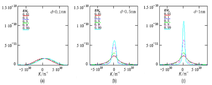
Figure 1: Illustrating the dependence of width of the momentum ($K\hbar$) distribution on $E/V_{0}$: (a) For the case of barrier thickness 0.1 nm the width of the momentum distribution nearly independent of $E/V_{0}$. (b) For the case of barrier thickness 0.5 nm the width of the momentum distribution decreasing with increasing of $E/V_{0}$. (c) For the case of barrier thickness 1 nm the width of the momentum distribution rapidly decreasing with increasing of $E/V_{0}$.

Fig.1(a) shows the width of the momentum distribution nearly independent of $E/V_{0}$ for the case of barrier thickness 0.1 nm. Fig.1(b) shows the width of the momentum distribution decreasing with increasing of $E/V_{0}$ for the case of barrier thickness 0.5 nm. Fig.1(c) shows the width of the momentum distribution rapidly decreasing with increasing of $E/V_{0}$ for the case of barrier thickness 1 nm.

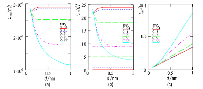
Figure 2: (a) The root-mean-square velocity ($v_{\textrm{\scriptsize{rms}}}$) dependent on the barrier thickness and $E/V_{0}$. (b) The effective tunneling kinetic energy dependent on the barrier thickness and $E/V_{0}$; the horizontal lines represent the incident kinetic energies. (c) The effective tunneling time dependent on the barrier thickness and $E/V_{0}$.

Fig.2(a) shows the root-mean-square velocity ($v_{\textrm{\scriptsize{rms}}}$) dependent on the barrier thickness and $E/V_{0}$. Fig.2(b) shows the effective tunneling kinetic energy ($\varepsilon_{\textrm{\scriptsize{eff}}}$) dependent on the barrier thickness and $E/V_{0}$. Fig.2(c) shows the effective tunneling time ($t_{\textrm{\scriptsize{eff}}}$) dependent on the barrier thickness and $E/V_{0}$.

The present definition of the tunneling time is completely different from the existing typical definitions, such as phase time [6,10], dwell time [7,10] and Bütticker-Landauer time [11]. According to the phase time definition, the tunneling time is supposed to be:

$$t_{\textrm{\scriptsize{ph}}}=\frac{d}{\sqrt{2E/m}}+\hbar\frac{\textrm{d}(\textrm{arg}S)}{\textrm{d}E}$$ (12)

Using Eq.4 and this equation for numerical calculation, we obtain the result as shown in Fig.3(a). Besides, according to the dwell time definition, the tunneling time is supposed to be:

$$t_{\textrm{\scriptsize{dw}}}=\frac{\int_{0}^{d}|\psi_{2}(x)|^{2}\textrm{d}x}{|J_{\textrm{in}}|}$$ (13)

Using Eq.2, Eq.8 and this equation for numerical calculation, we get the result as shown in Fig.3(b). These results are verified by using the following analytical expressions [10]:

$$t_{\textrm{\scriptsize{ph}}}=\frac{m}{\hbar k\kappa D}[2\kappa dk^{2}(\kappa^{2}-k^{2})+(\frac{2mV_{0}}{\hbar^{2}})^{2}\textrm{sinh}(2\kappa d)],~{}D=4\kappa^{2}k^{2}+(\frac{2mV_{0}}{\hbar^{2}})^{2}\textrm{sinh}^{2}(\kappa d)$$ (14)

$$t_{\textrm{\scriptsize{dw}}}=\frac{mk}{\hbar\kappa D}[2\kappa d(\kappa^{2}-k^{2})+\frac{2mV_{0}}{\hbar^{2}}\textrm{sinh}(2\kappa d)]$$ (15)

In Fig.3(a) and Fig.3(b) we see that the tunneling times are independent of the thickness of the thick barrier. This implies that the tunneling velocity may become even larger than the light velocity in vacuum since the barrier thickness may be arbitrary large. This kind of superluminal effect is referred to as Hartman effect. However, from Fig.2(a) we see no Hartman effect for the electron. Besides, Fig.3(c) shows Bütticker-Landauer time $t_{\textrm{\tiny{BL}}}=md/(\hbar\kappa)$ for an opaque barrier [11]. Clearly, the phase time, dwell time and Bütticker-Landauer time are contradictory to each other. The present author argues that all these tunneling times are not appropriate expressions for the actual transit time in a tunneling process.

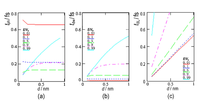
Figure 3: Graphic comparison of three typical tunneling times: (a) phase time , (b) dwell time, (c) Bütticker-Landauer time.

3 Time spent on penetration depth and Heisenberg’s energy-time uncertainty relation

We will shows that Heisenberg’s energy-time uncertainty relation is related to the time spent on penetration depth into the barrier which can be obtained from the relative probability density

$$D(x)=\frac{|\psi_{2}(x)|^{2}}{|\psi_{2}(0)|^{2}},~{}0\leq x\leq d$$ (16)

when its value reduces to $e^{-2}=0.135$ unless the barrier thickness is so small that it never reduces to this value in the barrier region in the case of 0.1 nm thickness as shown in Fig.4(a). For the cases $E/V_{0}$=0.01–0.99, the relative probability densities of the tunneling electron are shown in Fig.5(a)-(d). The wave function decays approximately exponentially as a function of x in the barrier region. The effective time spent on the penetration depth s is supposed to be

$$\tau_{\textrm{\scriptsize{eff}}}={s}/v_{\textrm{\scriptsize{rms}}}$$ (17)

Table 1 and Fig.5(a) show the penetration depths. Fig.5(b) shows the effective times ($\tau_{\textrm{\scriptsize{eff}}}$) spent on the penetration depths. The curves in Fig.5(c) show the introduced coefficient ($\xi$) in Heisenberg’s energy-time uncertainty relation, defined by the relation

$$\Delta E\Delta t=\xi\hbar/2,~{}\Delta E=\varepsilon_{\textrm{\scriptsize{eff}}},~{}\Delta t=\tau_{\textrm{\scriptsize{eff}}}$$ (18)

We see that for $E/V_{0}$=0.01–0.99 Heisenberg’s energy-time uncertainty relation is satisfied very well since $1.5<\xi\leq 5$ .

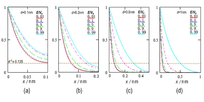
Figure 4: Relative probability densities of the tunneling electron in the barrier region for the cases: (a) barrier thickness 0.1 nm, (b) barrier thickness 0.2 nm, (c) barrier thickness 0.5 nm, (d) barrier thickness 1 nm. The horizontal line represents the value of $e^{-2}=0.135$.

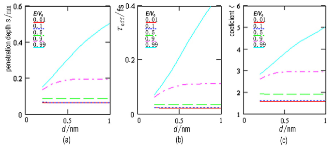
Figure 5: (a) The penetration depth of the electron in the barrier region. (b) The effective time spent on the penetration depth. (c) The coefficient in Heisenber’s energy-time uncertainty relation for verifying the relation.

	barrier thickness d (nm) and penetration depth s (nm)
$E/V_{0}$	d=0.2	d=0.3	d=0.4	d=0.5	d=0.6	d=0.7	d=0.8	d=0.9	d=1.0
0.01	0.0627	0.0621	0.0621	0.0621	0.0621	0.0621	0.0621	0.0621	0.0621
0.1	0.0658	0.0651	0.0651	0.0651	0.0651	0.0651	0.0651	0.0651	0.0651
0.5	0.0876	0.0874	0.0874	0.0874	0.0874	0.0874	0.0874	0.0874	0.0874
0.9	0.1357	0.1632	0.1811	0.1897	0.1933	0.1947	0.1952	0.1953	0.1954
0.99	0.1521	0.2012	0.2547	0.3069	0.3560	0.4011	0.4413	0.4767	0.5065

Table 1: Penetration depths of the tunneling electron in the barrier regions

4 High-jumping model of quantum tunneling

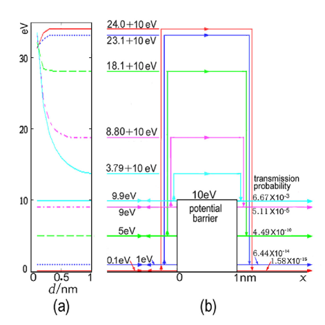
Figure 6: (a) The incident kinetic energy (horizontal line, 0.1–9.9 eV) and the effective kinetic energy plus the potential energy of the electron in the barrier region. (b) Illustration of quantum high-jumping model for the electron tunneling through the barrier of thickness 1 nm.

The quantum tunneling effect can be realistically explained by a high-jumping model for a quantum particle which has a certain chance to borrow enough energy from self-interference [8,9] to jump over a potential barrier as shown in Fig.6(b). We see that the less the incident kinetic energy of the electron is the higher it jumps until reaching a limit, for example, limit 34.102 eV for d=1 nm. In this high-jumping model, the kinetic energy is positive and the momentum is real in the classically forbidden potential barrier. On the contrary, it is widely accepted in literature that the former is negative and the latter is imaginary in the barrier. Realistically, the kinetic energy is never negative since both mass and velocity squared are always positive. The quantum high-jumping model demonstrates that the non-peaked part of the primary non-spreading wave packet describing a quantum particle plays a dramatic role in its self-interference.

5 Conclusion

There remains the old question of how long a quantum particle takes to tunnel through a potential barrier higher than its incident kinetic energy. In this article a solution of the question is proposed on the basis of a realistic explanation of quantum mechanics. The explanation implies that the tunneling particle has a certain chance to borrow enough energy from self-interference to high-jump over the barrier. The root-mean-square velocity and the effective tunneling time of an electron tunneling through a rectangular barrier are numerically calculated. No superluminal effect (Hartman effect) is found for the tunneling electron. Heisenberg’s energy-time uncertainty relation for the tunneling effect is verified by calculating an introduced coefficient representing uncertainty. The present author argues that phase time, dwell time and Bütticker-Landauer time are not appropriate expressions for the actual transit time in a tunneling process. A quantum high-jumping model is presented to resolve the paradox that kinetic energy of the tunneling particle is negative and its momentum is imaginary.

References

- [1] MacColl, L. A., Note on the transmission and reflection of wave packets by potential barriers, Phys. Rev. 40, 621 (1932).
- [2] Hartman, T. E., Tunneling of a wave packet, J. Appl. Phys. 33, 3427 (1962).
- [3] Hauge, E. H. and Støvneng, J. A., Tunneling times: A critical review, Rev. Mod. Phys. 61, 917 (1989).
- [4] Olkhovsky, V. S. and Recami, E., Tunneling and superluminal tunneling: A brief review, cond-mat/9802162.
- [5] Winful, H. G., Tunneling time, the Hartman effect, and superluminality: A proposed resolution of an old paradox, Phys. Rep. 436, 1-69 (2006).
- [6] Wigner, E. P., Lower limit for the energy derivation of the scattering phase time, Phys. Rev. 98, 145 (1955).
- [7] Smith, F. T., Lifetime matrix in collision theory, Phys. Rev. 118, 349 (1960).
- [8] Wang Guowen, Heuristic explanation of quantum interference experiments, quant-ph/0501148.
- [9] Wang Guowen, Finding way to bridge the gap between quantum and classical mechanics, physics/0512100.
- [10] Bütticker, M., Larmor precession and the traversal time for tunneling, Phys. Rev. B27, 6178 (1983).
- [11] Bütticker, M. and Landauer, R., Traversal time for tunneling, Phys. Rev. Lett. 49, 1739 (1982).