Coupled phantom field in loop quantum cosmology

Abstract

A model of phantom scalar field dark energy under exponential potential coupling to barotropic dark matter fluid in loop quantum cosmology is addressed here. We derive a closed-autonomous system for cosmological dynamics in this scenario. The expansion in loop quantum universe has a bounce even in presence of the phantom field. The greater decaying from dark matter to dark phantom energy results in greater energy storing in the phantom field. This results in further turning point of the field. Greater coupling also delays bouncing time. In the case of phantom decaying, oscillation in phantom density makes small oscillation in the increasing matter density.

I Introduction

There has recently been evidence of present accelerating expansion of the universe from cosmic microwave background (CMB) anisotropies, large scale galaxy surveys and type Ia supernovae Spergel:2003cb ; Scranton:2003in ; Riess:1998cb . Dark energy (DE) in form of either cosmological constant or scalar field matter is a candidate answer to the acceleration expansion which could not be explained in the regime of standard big bang cosmology Copeland:2006wr . DE possesses equation of state $p=w\rho$ with $w<-1/3$ enabling it to give repulsive gravity and therefore accelerate the universe. Combination of observational data analysis of CMB, Hubble Space Telescope, type Ia Supernovae and 2dF datasets allows constant $w$ value between -1.38 and -0.82 at the 95 % of confident level Melchiorri:2002ux . Meanwhile, assuming flat universe, the analysis result, $-1.06<w<-0.90$ has been reported by Spergel:2006hy using WMAP three-year results combined with Supernova Legacy Survey (SNLS) data. Without assumption of flat universe, mean value of $w$ is -1.06 (within a range of -1.14 to -0.93). Most recent data (flat geometry assumption) from ESSENCE Supernova Survey Ia combined with SuperNova Legacy Survey Ia gives a constraint of $w=-1.07\pm 0.09$ Wood-Vasey:2007jb . Observations above show a possibility that a fluid with $w<-1$ could be allowed in the universe Caldwell:1999ew . This type of cosmological fluid is dubbed phantom. Conventionally Phantom behavior arises from having negative kinetic energy term.

Dynamical properties of the phantom field in the standard FRW cosmology were studied before. However the scenario encounters singularity problems at late time Li:2003ft ; Urena-Lopez:2005zd . While investigation of phantom in standard cosmological model is still ongoing, there is an alternative approach in order to resolve the singularity problem by considering phantom field evolving in Loop Quantum Cosmology (LQC) background instead of standard general relativistic background Samart:2007xz ; Naskar:2007dn . Loop Quantum Gravity-LQG is a non-perturbative type of quantization of gravity and is background-independent Thiemann:2002nj ; Ashtekar:2003hd . LQG provides cosmological background evolution for LQC. An effect from loop quantum modification gives an extra correction term $-{\rho^{2}}/\rho_{\rm lc}$ into the standard Friedmann equation Bojowald:2001ep ; Date:2004zd ; Singh:2006sg . Problem for standard cosmology in domination of phantom field is that it leads to singularity, so called the Big Rip Caldwell:2003vq . The $-{\rho^{2}}/\rho_{\rm lc}$ term, when dominant at late time, causes bouncing of expansion hence solving Big Rip singularity problem Ashtekar:2003hd ; Bojowald:2001xe ; Ashtekar:2006rx . Recently, a general dynamics of scalar field including phantom scalar field coupled to barotropic fluid has been investigated in standard cosmological background. In this scenario, the scaling solution of the coupled phantom field is always unstable and it can not yield the observed value $\Omega_{\phi}\sim 0.7$ Gumjudpai:2005ry . Indeed there should be other effects from loop quantum correction to the Friedmann equation. Moreover when including potential term in scalar field density, the quantum modification must be included Bojowald:2006gr . Although, the Friedmann background is valid only in absence of field potential, however, investigation of a phantom field evolving under a potential could reveal some interesting features of the model. In this letter, we investigate a case of coupled phantom field in LQC background in alternative to the standard relativistic cosmology case. In Section II, we introduce framework of cosmological equations before considering dynamical autonomous equations in Section III. We show some numerical results in Section IV where the coupling strength is adjusted and compared. Conclusion and comments are in Section V.

II COSMOLOGICAL EQUATIONS

II.1 Loop quantum cosmology

The effective flat universe Friedmann equation from LQC is given as Bojowald:2001ep ; Singh:2006sg ,

$$H^{2} = \frac{\rho}{3M_{\rm P}^{2}}\left(1-\frac{\rho}{\rho_{\rm lc}}\right),$$ (1)

where $H$ is Hubble constant, $M_{\rm P}$ is reduced Planck mass, $\rho$ is density of cosmic fluid, $\rho_{\rm lc}=\sqrt{3}/(16\pi\zeta^{3}G^{2}\hbar)$. The parameter $\zeta$ is Barbero-Immirzi dimensionless parameter and $G$ is the Newton’s gravitational constant.

II.2 Phantom scalar field

Nature of the phantom field can be extracted from action,

$$S=\int{\rm d}^{4}x\sqrt{-g}\left[\frac{1}{2}(\partial^{a}\phi)(\partial_{a}\phi)-V(\phi)\right].$$ (2)

Energy density and pressure are given by

$$\rho_{\phi}=-\frac{1}{2}\dot{\phi}^{2}+V(\phi),$$ (3)

and

$$p_{\phi}=-\frac{1}{2}\dot{\phi}^{2}-V(\phi),$$ (4)

with equation of state,

$$w_{\phi}\equiv\frac{p_{\phi}}{\rho_{\phi}}=\frac{\dot{\phi}^{2}+2V(\phi)}{\dot{\phi}^{2}-2V(\phi)}.$$ (5)

When the field is slowly rolling, the approximate value of $w$ is -1. As long as the approximation, $\dot{\phi}^{2}\sim 0$ or the condition, $\dot{\phi}^{2}<2V$ holds, $w$ is always less than -1. In our scenario, the universe contains two fluid components. These are barotropic fluid with equation of state $p_{\rm m}=\rho_{\rm m}w_{\rm m}$ and phantom scalar field fluid. The total density is then $\rho=\rho_{\rm m}+\rho_{\phi}$ which governs total dynamics of the universe.

II.3 Coupled phantom scalar field

Here we consider both components coupling to each other. Fluid equations for coupled scalar fields proposed by Piazza:2004df assuming flat standard FRW universe are

$$\dot{\rho}_{\phi}+3H(1+w_{\phi})\rho_{\phi} = -Q\rho_{\rm m}\dot{\phi}\,,$$ (6)

$$\dot{\rho}_{\rm m}+3H(1+w_{\rm m})\rho_{\rm m} = +Q\rho_{\rm m}\dot{\phi}\,.$$ (7)

These fluid equations contain a constant coupling between dark matter (the barotropic fluid) and dark energy (the phantom scalar field) as in Amendola:1999er . Eqs. (6) and (7) can also be assumed as conservation equations of fluids in the LQC. Total action for matter and phantom scalar field is Piazza:2004df

$$S=\int{\rm d}^{4}x\sqrt{-g}\left[\frac{M_{\rm P}^{2}}{2}R+p(X,\phi)\right]+S_{\rm m}(\phi)\,.$$ (8)

Assuming scaling solution of the dark energy in standard cosmology, the pressure Lagrangian density is written as

$$p(X,\phi)=-X-c\exp(-\lambda\phi/M_{\rm P}^{2})\,,$$ (9)

where $X$ is the kinetic term, $-g^{ab}\partial_{a}\phi\partial_{b}\phi/2$ of the Lagrangian density (2) and (9). The second term on the right of Eq. (9) is exponential potential, $V(\phi)=c\exp(-\lambda\phi/M_{\rm P}^{2})$ which gives scaling solution for canonical and phantom ordinary scalar field in standard general relativistic cosmology when steepness of the potential, $\lambda$ is fine tuned as

$$\lambda=Q\frac{1+w_{\rm m}-\Omega_{\rm\phi}(w_{\rm m}-w_{\rm\phi})}{\Omega_{\rm\phi}(w_{\rm m}-w_{\rm\phi})}\,.$$ (10)

The steepness (10) is, in standard cosmological circumstance, constant in the scaling regime due to constancy of $w_{\phi}$ and $\Omega_{\phi}$ Piazza:2004df ; Gumjudpai:2005ry . However, in LQC case, there has been a report recently that the scaling solution does not exist for phantom field evolving in LQC Samart:2007xz . Therefore our spirit to consider constant $\lambda$ is the same as in Copeland:1997et not a motivation from scaling solution as in Piazza:2004df . The exponential potential is also originated from fundamental physics theories such as higher-order gravity highergrav or higher dimensional gravity string .

III COSMOLOGICAL DYNAMICS

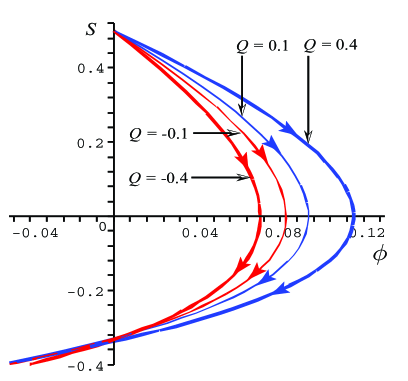
Figure 1: Phase portrait of $S(t)$ versus $\phi(t)$ for $Q=-0.4,-0.1,0.1$ and $0.4$ from left to right. All trajectories have the same initial conditions $S(0)=0.5$ and $\phi(0)=0$.

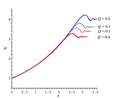
Figure 2: Scale factor plotted versus time for $Q=-0.4,-0.1,0.1$ and $0.4$ (from bottom to top).

Time derivative of the effective LQC Friedmann equation LQC (1) is

$$\dot{H} = -\frac{(\rho+p)}{2M_{\rm P}^{2}}\left(1-\frac{2\rho}{\rho_{\rm lc}}\right),$$ (13)

$$= -\frac{(1+w_{\phi})\rho_{\phi}+(1+w_{\rm m})\rho_{\rm m}}{2M_{\rm P}^{2}}\left[1-\frac{2}{\rho_{\rm lc}}(\rho_{\phi}+\rho_{\rm m})\right],$$

$$= -\frac{\left[-S^{2}+(1+w_{\rm m})\rho_{\rm m}\right]}{2M_{\rm P}^{2}}\times$$

$$\left[1-\frac{2}{\rho_{\rm lc}}\left(-\frac{S^{2}}{2}+ce^{-\lambda\phi/M_{\rm P}^{2}}+\rho_{\rm m}\right)\right].$$

In above equations we define new variable

$$S\equiv\dot{\phi}.$$ (14)

The coupled fluid equations (6) and (7) are re-expressed in term of $S$ as

$$\dot{S} = -3HS+\frac{{\rm d}V}{{\rm d}\phi}+Q\rho_{\rm m}\,,$$ (15)

$$\dot{\rho}_{\rm m} = -3H(1+w_{\rm m})\rho_{\rm m}+Q\rho_{\rm m}S\,.$$ (16)

The Eqs. (13), (14), (15) and (16) form a closed autonomous set of four equations. The variables here are $\rho_{\rm m}$, $S$, $\phi$ and $H$. The autonomous set recovers standard general relativistic cosmology in the limit $\rho_{\rm lc}\rightarrow\infty$. The general relativistic limit affects only the equation involving $H$. From the above autonomous set, one can do a qualitative analysis with numerical integration similar to phase plane presented in different situation Gumjudpai:2003vv . Another approach of analysis is to consider a quantitative analysis Gumjudpai2007 .

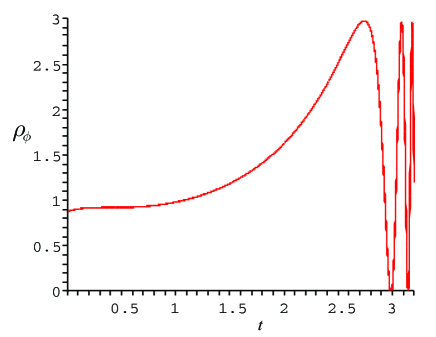
Figure 3: Phantom field density plotted versus time for $Q=-0.1$. The other values of $Q$ also yield bouncing and oscillation.

IV NUMERICAL SOLUTIONS

Here we present some numerical solution for a positive and negative coupling between the phantom field and barotropic fluid. The solutions presented here are physically valid solutions corresponding to Class II solutions characterized in Samart:2007xz . For non-minimally coupled scalar field in Einstein frame Uzan:1999ch , the coupling $Q$ lies in a range $-1/\sqrt{6}<Q<1/\sqrt{6}$. Here we set $Q=-0.4,-0.1,0.1$ and $0.4$ which lie in the range. Effect of the coupling can be seen from Eqs. (6) and (7). Negative $Q$ enhances decay rate of scalar field to matter while giving higher matter creation rate. On the other hand, positive $Q$ yields opposite result. Greater magnitude of $Q<0$ gives higher decay rate of the field to matter. Greater magnitude of $Q>0$ will result in higher production rate of phantom field from matter.

IV.1 Phase portrait

The greater $Q$ value results in greater value of the field turning point (see $\phi$-intercept in Fig. 1). The kinetic term $S(t)$ turns negative at the turning points corresponding to the field rolling down and then halting before rolling up the hill of exponential potential. When $Q$ is greater, the field can fall down further, hence gaining more total energy. The result agrees with the prediction of Eqs. (6) and (7).

IV.2 Scale factor

From Fig. 2, the bounce in scale factor occurs later for greater $Q$ value of which the phantom field production rate is higher. The field has more phantom energy to accelerate the universe in counteracting the effect of loop quantum (the bounce). For less positive $Q$, the phantom production rate is smaller, and for negative $Q$, the phantom decays. Therefore it has less energy for accelerating the expansion in counteracting with the loop quantum effect. This makes the bounce occurs sooner.

IV.3 Energy density

Time evolutions of energy density of the matter and the phantom field are presented in Figs. 3 and 5. If $Q>0$, the matter decays to phantom. This reduces density of matter. While for $Q<0$, the matter gains its density from decaying of phantom field. In Fig. 3 there is a bounce of phantom density before undergoing oscillation. For a non-coupled case, it has recently been reported that the phantom density also undergoes oscillation Samart:2007xz . As seen in Figs. 5 and 5, the oscillation in phantom density of the phantom decay case ($Q<0$) affects in oscillation in matter density while for the case of matter decay ($Q>0$), the matter density is reduced for stronger coupling. The oscillation in the phantom density comes from oscillation of the kinetic term $\dot{\phi}$, i.e. $S(t)$ as shown in Samart:2007xz .

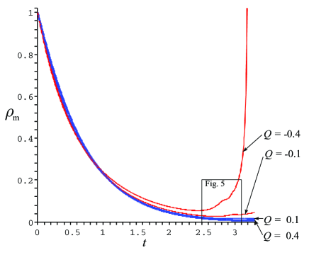
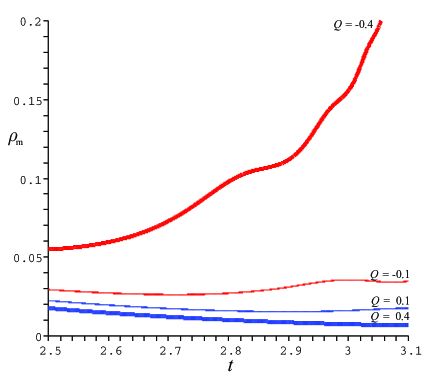
Figure 4: Matter density plotted versus time for $Q=-0.4,-0.1,0.1$ and $0.4$ (from top to bottom).

Figure 5: Zoom-in portion of Fig. 5. The phantom field decays to matter at highest rate for $Q=-0.4$ (top line). Oscillation in matter density due to oscillation in the phantom field density is seen clearly here.

V Conclusion and comments

In this letter, we have derived an autonomous system of a loop quantum cosmological equations in presence of phantom scalar field coupling to barotropic matter fluid. We choose constant coupling $Q$ between matter and the phantom field to positive and negative values and check numerically the effect of $Q$ values on (1) phase portrait, (2) scale factor and (3) energy density of phantom field and matter. We found that field value tends to roll up the hill of potential due to phantom nature. With greater $Q$, the field can fall down on the potential further. This increases total energy of the field. For canonical scalar field either standard or phantom, LQC yields a bounce. The bounce is useful since it is able to avoid Big Bang singularity in the early universe. Here our numerical result shows a bouncing in scale factor at late time. This is a Type I singularity avoidance even in presence of phantom energy. The greater coupling results in more and more phantom density. Greater phantom effect therefore delays the bounce, which is LQC effect, to later time. In the case of matter decay to phantom ($Q>0$), oscillation in phantom energy density does not affect matter density. On the other hand, when $Q<0$, phantom decays to matter, oscillation in phantom density results in oscillation in the increasing matter density.

This work considers only the effects of sign and magnitude of the coupling constant to qualitative dynamics and evolution of the system. Studies of field dependent effects of coupling $Q(\phi)$ in some scalar-tensor theory of gravity and investigation of an evolution of effective equation of state could also yield further interesting features of the model. Quantitative dynamical analysis of the model under different types of potential is also motivated for future work. Frequency function of the oscillation in scale factor and phantom density are still unknown in coupled case. It looks like that the oscillation frequency tends to increase. This could lead to infinite frequency of oscillation which is another new singularity.

Acknowledgements: B. G. is grateful to Shinji Tsujikawa for discussion. This work was presented as an invited talk at the SIAM Physics Congress 2007. B. G. thanks Thiraphat Vilaithong and the committee of the Thai Physics Society for an invitation to present this work at the congress. This work is supported by a TRF-CHE Research Career Development Grant of the Thailand Research Fund and the Royal Thai Government’s Commission on Higher Education.

References

- (1) C. L. Bennett et al., Astrophys. J. Suppl. 148, 1 (2003) [arXiv:astro-ph/0302207]; D. N. Spergel et al. [WMAP Collaboration], Astrophys. J. Suppl. 148 (2003) 175 [arXiv:astro-ph/0302209]; S. Masi et al., Prog. Part. Nucl. Phys. 48, 243 (2002) [arXiv:astro-ph/0201137].
- (2) R. Scranton et al. [SDSS Collaboration], [arXiv:astro-ph/0307335].
- (3) A. G. Riess et al. [Supernova Search Team Collaboration], Astron. J. 116, 1009 (1998) [arXiv:astro-ph/9805201]; A. G. Riess, arXiv:astro-ph/9908237; J. L. Tonry et al. [Supernova Search Team Collaboration], Astrophys. J. 594, 1 (2003) [arXiv:astro-ph/0305008]; S. Perlmutter et al. [Supernova Cosmology Project Collaboration], Astrophys. J. 517, 565 (1999) [arXiv:astro-ph/9812133]; G. Goldhaber et al. [The Supernova Cosmology Project Collaboration], arXiv:astro-ph/0104382.
- (4) E. J. Copeland, M. Sami and S. Tsujikawa, Int. J. Mod. Phys. D 15, 1753 (2006) [arXiv:hep-th/0603057]; T. Padmanabhan, Curr. Sci. 88, 1057 (2005) [arXiv:astro-ph/0411044]; T. Padmanabhan, AIP Conf. Proc. 861, 179 (2006) [arXiv:astro-ph/0603114].
- (5) A. Melchiorri, L. Mersini-Houghton, C. J. Odman and M. Trodden, Phys. Rev. D 68, 043509 (2003) [arXiv:astro-ph/0211522].
- (6) D. N. Spergel et al., arXiv:astro-ph/0603449.
- (7) W. M. Wood-Vasey et al., arXiv:astro-ph/0701041.
- (8) R. R. Caldwell, Phys. Lett. B 545, 23 (2002) [arXiv:astro-ph/9908168].
- (9) J. g. Hao and X. z. Li, Phys. Rev. D 67, 107303 (2003) [arXiv:gr-qc/0302100]; P. Singh, M. Sami and N. Dadhich, Phys. Rev. D 68, 023522 (2003) [arXiv:hep-th/0305110]; X. z. Li and J. g. Hao, Phys. Rev. D 69, 107303 (2004) [arXiv:hep-th/0303093]; J. G. Hao and X. z. Li, Phys. Rev. D 70, 043529 (2004) [arXiv:astro-ph/0309746]; M. Sami and A. Toporensky, Mod. Phys. Lett. A 19, 1509 (2004) [arXiv:gr-qc/0312009].
- (10) L. A. Urena-Lopez, JCAP 0509, 013 (2005) [arXiv:astro-ph/0507350].
- (11) D. Samart and B. Gumjudpai, arXiv:0704.3414 [gr-qc].
- (12) T. Naskar and J. Ward, arXiv:0704.3606 [gr-qc].
- (13) T. Thiemann, Lect. Notes Phys. 631, 41 (2003) [arXiv:gr-qc/0210094]; A. Perez, arXiv:gr-qc/0409061.
- (14) A. Ashtekar, M. Bojowald and J. Lewandowski, Adv. Theor. Math. Phys. 7, 233 (2003) [arXiv:gr-qc/0304074].
- (15) M. Bojowald, Class. Quant. Grav. 18, L109 (2001) [arXiv:gr-qc/0105113]; K. Vandersloot, Phys. Rev. D 71, 103506 (2005) [arXiv:gr-qc/0502082]; P. Singh and K. Vandersloot, Phys. Rev. D 72, 084004 (2005) [arXiv:gr-qc/0507029]; M. Bojowald, Living Rev. Rel. 8, 11 (2005) [arXiv:gr-qc/0601085].
- (16) G. Date and G. M. Hossain, Class. Quant. Grav. 21, 4941 (2004) [arXiv:gr-qc/0407073]; A. Ashtekar, T. Pawlowski and P. Singh, Phys. Rev. D 73, 124038 (2006) [arXiv:gr-qc/0604013]; G. M. Hossain, Class. Quant. Grav. 21, 179 (2004) [arXiv:gr-qc/0308014]; K. Banerjee and G. Date, Class. Quant. Grav. 22, 2017 (2005) [arXiv:gr-qc/0501102].
- (17) P. Singh, Phys. Rev. D 73, 063508 (2006) [arXiv:gr-qc/0603043]; A. Ashtekar, AIP Conf. Proc. 861, 3 (2006) [arXiv:gr-qc/0605011].
- (18) R. R. Caldwell, M. Kamionkowski and N. N. Weinberg, Phys. Rev. Lett. 91, 071301 (2003) [arXiv:astro-ph/0302506]; S. Nesseris and L. Perivolaropoulos, Phys. Rev. D 70, 123529 (2004) [arXiv:astro-ph/0410309]; J. D. Barrow, Class. Quant. Grav. 21, L79 (2004) [arXiv:gr-qc/0403084]; S. Nojiri, S. D. Odintsov and S. Tsujikawa, Phys. Rev. D 71, 063004 (2005) [arXiv:hep-th/0501025].
- (19) M. Bojowald, Phys. Rev. Lett. 86, 5227 (2001) [arXiv:gr-qc/0102069]; M. Bojowald, G. Date and K. Vandersloot, Class. Quant. Grav. 21, 1253 (2004) [arXiv:gr-qc/0311004]; G. Date, Phys. Rev. D 71, 127502 (2005) [arXiv:gr-qc/0505002].
- (20) A. Ashtekar, T. Pawlowski and P. Singh, Phys. Rev. Lett. 96, 141301 (2006) [arXiv:gr-qc/0602086]; M. Sami, P. Singh and S. Tsujikawa, arXiv:gr-qc/0605113.
- (21) B. Gumjudpai, T. Naskar, M. Sami and S. Tsujikawa, JCAP 0506, 007 (2005) [arXiv:hep-th/0502191].
- (22) M. Bojowald, Phys. Rev. D 74, 081301 (2007) [arXiv:gr-qc/0608100]; M. Bojowald, arXiv:gr-qc/0703144; M. Bojowald, arXiv:0705.4398 [gr-qc].
- (23) F. Piazza and S. Tsujikawa, JCAP 0407, 004 (2004) [arXiv:hep-th/0405054]; S. Tsujikawa and M. Sami, Phys. Lett. B 603, 113 (2004) [arXiv:hep-th/0409212].
- (24) L. Amendola, Phys. Rev. D 62, 043511 (2000) [arXiv:astro-ph/9908023].
- (25) E. J. Copeland, A. R. Liddle and D. Wands, Phys. Rev. D 57, 4686 (1998) [arXiv:gr-qc/9711068]; T. Barreiro, E. J. Copeland and N. J. Nunes, Phys. Rev. D 61, 127301 (2000) [arXiv:astro-ph/9910214]; S. C. C. Ng, N. J. Nunes and F. Rosati, Phys. Rev. D 64, 083510 (2001) [arXiv:astro-ph/0107321].
- (26) B. Whitt, Phys. Lett. 145B, 176 (1984); J. D. Barrow and S. Cotsakis, Phys. Lett. 214B, 515 (1988); D. Wands, Class. Quantum Grav. 11, 269 (1994).
- (27) M. B. Green, J. H. Schwarz and E. Witten, Superstring Theory, Cambridge University Press (1987).
- (28) B. Gumjudpai, Gen. Rel. Grav. 36, 747 (2004) [arXiv:gr-qc/0308046].
- (29) B. Gumjudpai, in preparation.
- (30) J. P. Uzan, Phys. Rev. D 59, 123510 (1999) [arXiv:gr-qc/9903004]; T. Chiba, Phys. Rev. D 60, 083508 (1999) [arXiv:gr-qc/9903094]; N. Bartolo and M. Pietroni, Phys. Rev. D 61, 023518 (2000) [arXiv:hep-ph/9908521].