Current Renormalization in Finite Volume

Abstract

For finite volume field theories with discrete translational invariance, conserved currents can be additively renormalized by infrared effects. We demonstrate this for pions using chiral perturbation theory coupled to electromagnetism in a periodic box. Gauge invariant single particle effective theories are constructed to explain these results. In such theories, current renormalization arises from operators involving the zero mode of the gauge field. No contradictions with Ward identities, or low-energy theorems are encountered.

I Introduction

Since Wilson’s pioneering work Wilson (1974), there has been considerable activity to solve field theories non-perturbatively by numerical simulation on Euclidean spacetime lattices. Today lattice gauge theory is a mature field, and current state-of-the-art lattice QCD calculations are beginning to confront the challenges provided by the hadron spectrum. For an overview of lattice methods, see DeGrand and DeTar (2006). One aspect to these numerical simulations is the finite-size scaling of observables. The finite spacetime volume employed on the lattice is a source of systematic error in the numerical determination of observables. Thus the study of field theories in finite volume, while a theoretical curiosity, is also of practical utility.

Recent work Detmold et al. (2006) suggests that electromagnetically gauge invariant amplitudes at finite volume may differ from their infinite volume form. Specifically investigated was the finite-size scaling of nucleon electromagnetic and spin polarizabilities that arise in nucleon Compton scattering (see, e.g., Hyde-Wright and de Jager (2004); Schumacher (2005)). A goal in Detmold et al. (2006) was to address systematic errors in the extraction of polarizabilities from classical background field methods employed in lattice simulations Fucito et al. (1982); Martinelli et al. (1982); Bernard et al. (1982); Fiebig et al. (1989); Aoki and Gocksch (1989); Aoki et al. (1990); Burkardt et al. (1996); Christensen et al. (2005); Detmold (2005); Lee et al. (2006); Shintani et al. (2007). An analysis of the finite volume behavior of nucleon polarizabilities was presented, as was an oddity relating to the zero-frequency scattering amplitude. In infinite volume, the zero-frequency Compton amplitude is fixed by gauge invariance to be proportional to the total charge squared. Finite volume modifications, however, were found for nucleon Compton scattering at zero frequencies Detmold et al. (2006). These results suggest a finite volume renormalization of the basic interaction between the photon and the hadron’s charge. In this work, we show that gauge invariance in finite volume allows for such modifications to zero-frequency photon couplings. In essence, conserved currents are not protected from additive renormalization as they are in infinite volume. For definiteness, we focus on the chiral dynamics of pions coupled to photons Gasser and Leutwyler (1984), but could just as well choose any interacting field theory coupled to gauge fields.

Our presentation is organized as follows. First in Sec. II, we analyze the electromagnetic interactions of pions in finite volume. We demonstrate the infrared running of electromagnetic current matrix elements by explicit one-loop calculations in chiral perturbation theory ($\chi$PT). In Sec. III, consequences of gauge invariance on a torus are detailed. Gauge invariant zero-mode interactions allow for infrared renormalization of electromagnetic couplings. We write down gauge invariant, zero-frequency effective field theories for pions that reproduce our one-loop finite volume $\chi$PT results. Understanding such volume effects is necessary in practice for the extraction of infinite volume physics from lattice QCD simulations. We show how our results are consistent with Ward identities and low-energy theorems in Sec. IV. A conclusion in Sec. V summarizes our findings, while a glossary of finite volume functions is provided in the Appendix.

II Pions in Finite Volume

The chiral Lagrangian is written in terms of a coset field $\Sigma=\exp(2i\Phi/f)$ which parametrizes the Goldstone manifold arising from spontaneous chiral symmetry breaking: $SU(2)_{L}\otimes SU(2)_{R}\to SU(2)_{V}$. The pions are contained in the matrix $\Phi$, explicitly as

$$\Phi=\begin{pmatrix}\frac{1}{\sqrt{2}}\pi^{0}&\pi^{+}\\ \pi^{-}&-\frac{1}{\sqrt{2}}\pi^{0}\end{pmatrix}.$$ (1)

In our conventions, the dimensionful parameter $f=132\,\texttt{MeV}$. The chiral Lagrangian provides an effective theory of low-energy QCD. At leading-order in an expansion in momentum, $p^{2}$, and quark mass, $m_{q}$, there are two terms in this Lagrangian

$${\mathcal{L}}=\frac{f^{2}}{8}\text{tr}\left(D_{\mu}\Sigma D^{\mu}\Sigma^{\dagger}\right)+\frac{f^{2}}{4}\lambda\,\text{tr}\left(\Sigma m_{q}+\Sigma^{\dagger}m_{q}\right),$$ (2)

where $m_{q}$ is the quark mass matrix, $m_{q}=\text{diag}(m_{u},m_{d})$. We shall work exclusively in the isospin limit, $m_{u}=m_{d}\equiv m$. The kinetic term of the chiral Lagrangian includes a $U(1)$ gauge covariant derivative that couples pions to photons, $D_{\mu}\Sigma=\partial_{\mu}\Sigma+ieA_{\mu}\left[Q,\Sigma\right]$, where the quark electric charge matrix, $Q$, is given by $Q=\text{diag}(2/3,-1/3)$.

Expanding the Lagrangian in Eq. (2) to tree level, one sees that the pions are correctly normalized and their mass, $m_{\pi}$, is given by $m_{\pi}^{2}=2\lambda m$. The couplings of pions to zero-momentum photons at tree level can be read off from Eq. (2), from which we find their canonical charges. We now investigate whether loop corrections in a finite spatial volume modify these couplings.

II.1 Charged pion current

To consider the one-loop corrections to the electromagnetic current of charged pions, we accordingly expand the $\chi$PT Lagrangian in Eq. (2) to second order to generate vertices for one-loop graphs. Furthermore local terms at higher-order can then contribute at tree-level, but these are absent for zero-frequency photons. Thus we need to determine only the diagrams depicted in Fig. 1.

               

Figure 1: One-loop graphs required to evaluate the pion electromagnetic current. On the left appears the wavefunction correction; while, on the right, diagrams contributing to the pion form factor. Vertices shown are generated from the leading-order $\chi$PT Lagrangian, Eq. (2).

In the limit of zero frequency and infinite volume, the current matrix element between charged pion states is required by gauge and Lorentz invariance to be

$$\langle\pi^{\pm}(P)|J_{\mu}|\pi^{\pm}(P)\rangle=\pm 2eP_{\mu},$$ (3)

where the overall sign reflects the charge of the pion. It is a straightforward exercise to verify the above form at one-loop order in infinite volume. At an intermediate step, we reach the result

$$\langle\pi^{\pm}(P)|J_{\mu}|\pi^{\pm}(P)\rangle=\pm 2e\left\{P_{\mu}-\frac{2i}{f^{2}}\int\frac{d^{4}q}{(2\pi)^{4}}\frac{(q^{2}-m_{\pi}^{2})P_{\mu}-2(q\cdot P)q_{\mu}}{[q^{2}-m_{\pi}^{2}]^{2}}\right\},$$ (4)

from which we see the wavefunction correction to the tree-level vertex is exactly canceled by the loop contributions to the form factor at zero frequency Gasser and Leutwyler (1985). In this way, the matter fields do not contribute to the running of the coupling and Eq. (3) is preserved.

In finite volume, we repeat the calculation of the pion current to one-loop order. We consider each of the three spatial directions of finite length $L$, and the quark fields subjected to boundary conditions that maintain discrete translational invariance. For definiteness, we assume periodic boundary conditions. As the pions are point-like objects in the effective theory, they satisfy the same boundary conditions as the point-like interpolating field $\Phi(x)\sim{\overline{q}}(x)\gamma_{5}q(x)$. Pions are hence also periodic with quantized spatial momentum modes of the form

$$\bm{q}=\frac{2\pi}{L}\bm{n},$$ (5)

where $\bm{n}$ is a triplet of integers. To keep matters simple, we keep the temporal extent infinite as is commonly done to determine finite-size effects for lattice QCD observables. To evaluate the pion current, we use the finite volume theory defined by Eq. (2). The loop diagrams shown in Fig. 1 are again generated. The only difference compared to infinite volume is that the spatial momenta of real and virtual states are quantized. The finite and infinite volume theories share exactly the same ultraviolet divergences, so we can calculate the finite volume effect by matching the two theories in the infrared. For an observable $X$ calculated in both finite, $X(L)$, and infinite, $X(\infty)$, volumes, we have

$$X(L)=X(\infty)+\Delta X(L),$$ (6)

where the matching term, $\Delta X(L)$, is free from ultraviolet divergences and gives the finite volume effect.

Returning to Eq. (4), we can carry out the finite volume matching, Eq. (6), for the pion current. We find

$$\langle\pi^{\pm}(P)|J_{\mu}|\pi^{\pm}(P)\rangle=\pm 2eP_{\mu}\left\{1-\frac{\delta_{\mu j}}{3f^{2}}\left[2\,I_{1/2}(m^{2}_{\pi},L)+m_{\pi}^{2}I_{3/2}(m^{2}_{\pi},L)\right]\right\},$$ (7)

where $I_{{\beta}}(m^{2},L)$ is defined in the Appendix. Results are consistent with charge conjugation invariance and the current is only modified in the spatially finite directions. Specifically the virtual pion cloud in finite volume screens the current of the infinite volume pion. In Fig. 2, we plot the finite volume modification to the pion current. Here the relative difference in the current matrix element at finite volume versus infinite volume, $\Delta J_{\pi^{+}}$, given by

$$\Delta J_{\pi^{+}}=\frac{\langle\pi^{+}(P)|\hat{\bm{e}}\cdot\bm{J}|\pi^{+}(P)\rangle_{L}-\langle\pi^{+}(P)|\hat{\bm{e}}\cdot\bm{J}|\pi^{+}(P)\rangle_{\infty}}{\langle\pi^{+}(P)|\hat{\bm{e}}\cdot\bm{J}|\pi^{+}(P)\rangle_{\infty}},$$ (8)

is plotted as a function of the length $L$ of the spatial dimension. We have used a unit vector $\hat{\bm{e}}$ to project onto the spatial part of the current. Accordingly the pion cannot be at rest, $\bm{P}\neq\bm{0}$. Subscripts on matrix elements denote the box size, with infinity corresponding to infinite volume.

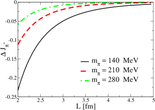
Figure 2: Finite volume screening of the pion current. The relative difference in pion current $\Delta J_{\pi^{+}}$ is plotted as a function of the box size $L$, for a few values of the pion mass.

The finite volume effect is exponentially suppressed in asymptotic ($m_{\pi}L\gg 1$) volumes. Consequently taking the infrared cutoff, $1/L$, to zero, the additive current renormalization vanishes and infinite volume limit is maintained.

II.2 Neutral pion current matrix elements

Charge conjugation invariance demands the identical vanishing of single current matrix elements between neutral pion states. Indeed whether the calculation of the neutral pion current is carried out in infinite or finite volume, we find zero for the matrix element. The $SU(2)$ flavor structure of the form factor diagrams shown in Fig. 1 ensures this vanishing and consistency with charge conjugation.

Neutral pion matrix elements of an even number of electromagnetic currents, however, are not restricted to vanish by charge conjugation invariance. Indeed, it is well known that the neutral pion has electric and magnetic polarizabilities that can be predicted at one-loop order in $\chi$PT solely in terms of $f$ and $m_{\pi}$ Holstein (1990). Such polarizabilities arise at second order in the low-frequency expansion of the matrix element of two currents (the so-called Compton scattering tensor). The Compton tensor also has a term at zeroth order in the photon frequencies

$$T_{\mu\nu}(\omega=\omega^{\prime}=0)=2(Qe)^{2}g_{\mu\nu},$$ (9)

which is sensitive only to the longest ranged electromagnetic interaction. This term in the Compton tensor, when combined with relevant phase space factors, yields the classical Thomson scattering cross section, $\sigma=8\pi(Qe)^{4}/3m^{2}_{\pi}$. For the neutral pion, the total charge is zero and the longest ranged interaction vanishes.

Figure 3: One-loop contributions to neutral pion Compton scattering in $\chi$PT. Vertices shown are generated from the leading-order Lagrangian.

Using the $\chi$PT Lagrangian defined in Eq. (2), we can determine the Compton amplitude for pions. We restrict our attention to the zero-frequency amplitude. Due to charge neutrality, there are no tree-level couplings to the neutral pion. At one-loop order, evaluation of the diagrams shown in Fig. 3 is required to determine the Compton amplitude. At an intermediate step in the calculation, contributions from all six diagrams can be simplified to

$$T_{\mu\nu}(\omega=\omega^{\prime}=0)=\frac{4ie^{2}m_{\pi}^{2}}{f^{2}}\int\frac{d^{4}q}{(2\pi)^{4}}\frac{(q^{2}-m_{\pi}^{2})g_{\mu\nu}-4q_{\mu}q_{\nu}}{[q^{2}-m_{\pi}^{2}]^{3}},$$ (10)

which vanishes. Hence in infinite volume, a delicate cancellation between all diagrams maintains the vanishing of the Compton amplitude at zero frequency Bijnens and Cornet (1988); Donoghue et al. (1988). On the other hand, the same is not true in finite volume. Carrying out the one-loop matching between finite and infinite volume theories, Eq. (6), for the Compton amplitude in Eq. (10), we find

$$T_{\mu\nu}(\omega=\omega^{\prime}=0)=e^{2}(\delta_{\mu 0}\delta_{\nu 0}-g_{\mu\nu})\frac{m_{\pi}^{4}}{f^{2}}\,I_{5/2}(m^{2}_{\pi},L).$$ (11)

Thus when one considers the purely spatial components of the Compton tensor, the neutral pion has an effective charge-squared, cf. Eq. (9).

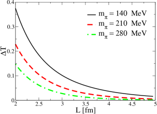
Figure 4: Zero frequency Compton amplitude for the neutral pion. The finite volume amplitude $\Delta T$ is plotted as a function of the box size $L$, for a few values of the pion mass. In infinite volume, this amplitude is identically zero.

In transverse gauge, the above expression gives the amplitude to scatter zero-frequency photons off the neutral pion. There is a non-vanishing contribution to this scattering amplitude when the pion is confined to a periodic box with size on the order of the pion Compton wavelength. When the box size becomes large compared to this scale, the amplitude is exponentially suppressed and infinite volume results are recovered. We demonstrate this in Fig. 4, where we plot the finite volume amplitude $\Delta T$ defined by

$$\Delta T=-\frac{1}{3e^{2}}g^{\mu\nu}T_{\mu\nu}(\omega=\omega^{\prime}=0).$$ (12)

III Gauge invariance on a torus

To explain our above results, we investigate electromagnetism in finite volume. The analogous finite temperature case is well known and described, e.g., in Zinn-Justin (1996). Because our applications are with classical background fields, or equivalently current operator insertion methods in lattice field theory, there are no quantum corrections to the photon field itself.

III.1 Spatial Torus

Let us consider a classical electromagnetic field defined on a finite spatial torus with infinite time extent. On the gauge field $A_{\mu}(\bm{x},t)$, we impose periodic boundary conditions and expand $A_{\mu}(\bm{x},t)$ in Fourier modes

$$A_{\mu}(\bm{x},t)=\sum_{\bm{n}}\tilde{A}_{\mu}(\bm{n},t)\,e^{2\pi i\bm{n}\cdot\bm{x}/L},$$ (13)

where $\bm{n}=(n_{x},n_{y},n_{z})\in\mathbb{Z}^{3}$. It is convenient to separate out the zero-mode contribution, so we write

$$A_{\mu}(\bm{x},t)={\mathcal{A}}_{\mu}(t)+{\overline{A}}_{\mu}(\bm{x},t),$$ (14)

where the zero mode ${\mathcal{A}}_{\mu}(t)\equiv\tilde{A}_{\mu}(\bm{0},t)$.

Under a gauge transformation, the photon field transforms in the familiar way, $A_{\mu}(\bm{x},t)\longrightarrow A_{\mu}(\bm{x},t)+\partial_{\mu}\alpha(\bm{x},t)$, and observables are invariant. Requiring the gauge transformed field to be single valued mandates that $\partial_{\mu}\alpha(\bm{x},t)$ is periodic. Thus we can decompose the gauge function $\alpha(\bm{x},t)$ into the sum of two terms, $\alpha(\bm{x},t)=\alpha_{0}(\bm{x},t)+{\overline{\alpha}}(\bm{x},t)$, where

$$\alpha_{0}(\bm{x},t)=\alpha_{0}(t)+\bm{\alpha}\cdot\bm{x},$$ (15)

and

$${\overline{\alpha}}(\bm{x},t)=\sum_{\bm{m}\neq\bm{0}}{\overline{{\tilde{\alpha}}}}(\bm{m},t)\,e^{2\pi i\bm{m}\cdot\bm{x}/L}.$$ (16)

Here we have dropped all overall irrelevant constants, and the vector $\bm{\alpha}$ is a constant vector. Using this decomposition for the gauge function, the gauge field transforms as

$$\begin{cases}{\mathcal{A}}_{\mu}(t)&\longrightarrow{\mathcal{A}}_{\mu}(t)+\partial_{\mu}\alpha_{0}(\bm{x},t)\\ {\overline{A}}_{\mu}(\bm{x},t)&\longrightarrow{\overline{A}}_{\mu}(\bm{x},t)+\partial_{\mu}{\overline{\alpha}}(\bm{x},t)\end{cases}.$$ (17)

In particular, the photon zero-mode transforms as

$${\mathcal{A}}_{\mu}(t)\longrightarrow{\mathcal{A}}_{\mu}(t)+\begin{cases}\partial_{0}\alpha_{0}(t),&\mu=0\\ \alpha_{i},&\mu=i\end{cases}.$$ (18)

The time-component of the zero mode is absent from the field strength tensor. The remaining three components of the zero mode field are translated by a constant under the gauge transformation. In the gauge invariant free theory, each spatial component of the zero mode is thus a massless one-dimensional scalar.

III.2 Coupling to Matter

For a generic matter field $\varphi(\bm{x},t)$ of unit charge, the effects of a gauge transformation show up as a local phase factor

$$\varphi(\bm{x},t)\longrightarrow\varphi^{\prime}(\bm{x},t) = e^{-i\alpha(\bm{x},t)}\varphi(\bm{x},t).$$ (19)

Now we assume that the matter field $\varphi(\bm{x},t)$ is subject to periodic boundary conditions. We again split the gauge function into zero mode and non-zero mode pieces, $\alpha(\bm{x},t)=\alpha_{0}(\bm{x},t)+{\overline{\alpha}}(\bm{x},t)$. With the form given in Eq. (16), we see that the non-zero modes will maintain the periodicity of the matter field under the transformation in Eq. (19). The same is not in general true of the zero modes given the form of ${\alpha}_{0}(\bm{x},t)$ in Eq. (15). If the gauge transformed matter field is to remain periodic under translations by $L$, then we must have the quantization condition

$$\bm{\alpha}=\frac{2\pi}{L}\bm{n},$$ (20)

on the spatial zero mode part of the gauge function. This quantization condition reduces the continuous translational invariance of the spatial zero modes to discrete translations. As gauge transformations are now less general compared to infinite volume, more gauge invariant operators can be built.

Imagine that we start with some microscopic theory with electromagnetic interactions. Take the scalar field $\varphi(\bm{x},t)$ as some composite low-energy degree of freedom of this theory. Further we assume that the energies of interest are ultra-low in the sense that any interactions of $\varphi(\bm{x},t)$ with itself or other fields have been integrated out. In the absence of electromagnetism, e.g., we have a simple single particle effective theory

$${\mathcal{L}}=|\partial_{\mu}\varphi|^{2}-m(L)^{2}|\varphi|^{2},$$ (21)

where $m(L)$ is a running mass that depends on the infrared cutoff $1/L$ (and parametrically depends on the other couplings, masses, etc. that have been integrated out of the theory). Running the cutoff to zero completes the infrared sector of the theory and produces infinite volume physics.

Now we include electromagnetism in this single particle effective theory by adding all possible gauge invariant operators. The minimal coupling prescription, $\partial_{\mu}\to D_{\mu}=\partial_{\mu}+iA_{\mu}$, renders the kinetic term of Eq. (21) gauge invariant. Because we imagine $\varphi$ is a composite particle, there can be non-minimal couplings that respect gauge invariance, e.g., the $\bm{E}^{2}$ and $\bm{B}^{2}$ terms for the particle’s polarizabilities. Further terms in this ultra low-energy theory are allowed, however, because $SO(4)$ is not respected, and the gauge invariance of the zero mode has a special nature. As we will show, these further terms are responsible for current renormalization. To simplify the discussion, we will restrict ourselves to the effective theory operators for zero frequency photons.

Using gauge symmetry, we can write down the general form of the ultra low-energy effective theory for a single $\varphi$ field coupled to zero frequency photons. We choose to construct this theory using Wilson lines. By cycling once over the $i$-th compact dimension, we can form gauge invariant Wilson lines ${\mathcal{W}}_{i}$ of the form,

$${\mathcal{W}}_{i}=\exp\left(i\oint dx_{i}\,A_{i}\right).$$ (22)

Notice that there is no sum over repeated indices in this definition. Due to the periodicity of the gauge field in the $i$-th direction, the loop integral

$$\int_{0}^{L}dx_{i}\,A_{i}(\bm{x},t)=L\mathcal{A}_{i}(t)+L\sum_{n_{j\neq i},\,n_{i}=0}\tilde{A}_{i}(\bm{n},t)e^{2\pi i\bm{n}\cdot\bm{x}/L},$$ (23)

produces just the $n_{i}=0$ modes of the gauge field. Indeed the gauge transformation of the zero and non-zero modes, Eq. (17), demonstrates that the Wilson line ${\mathcal{W}}_{i}$ is gauge invariant. For our purpose, we wish to isolate completely the gauge field zero-mode and accordingly form modified Wilson lines $W_{i}$ given by

$$W_{i}={\mathcal{P}}_{\bm{0}}{\mathcal{W}}_{i}{\mathcal{P}}_{\bm{0}}^{\dagger},$$ (24)

where ${\mathcal{P}}_{\bm{0}}$ is an operator that projects onto the zero-mode of the gauge field. A practical way to implement the action of ${\mathcal{P}}_{\bm{0}}$ is to change the loop integration

$$\oint dx_{i}\longrightarrow\frac{1}{L^{2}}\oint\prod_{j=1}^{3}dx_{j}\equiv\frac{1}{L^{2}}\oint d\bm{x}$$ (25)

so that

$$W_{i}=\exp\left(i\oint d\bm{x}\,A_{i}/L^{2}\right).$$ (26)

Furthermore it is useful to define Hermitian combinations of modified Wilson lines that transform simply under parity and charge conjugation,

$$W^{(+)}_{i} = \frac{1}{2}\left(W_{i}+W_{i}^{\dagger}\right)$$ (27)

$$W^{(-)}_{i} = \frac{1}{2i}\left(W_{i}-W_{i}^{\dagger}\right).$$ (28)

Notice that because $W_{i}^{(+)}=\sqrt{1-[W_{i}^{(-)}]^{2}}$, any operator involving $W_{i}^{(+)}$ can be traded in for a tower of operators involving $W_{i}^{(-)}$. Hence we can build our theory solely in terms of $W_{i}^{(-)}$ operators.

In addition to gauge, $C$, $P$, and $T$ invariance, the theory on a torus has $S_{4}$ cubic invariance. Writing down operators consistent with these symmetries, we arrive at the following ultra low-energy effective Lagrangian for a single $\varphi$ field

$${\mathcal{L}} = |D_{\mu}\varphi|^{2}-m(L)^{2}|\varphi|^{2}+{\mathcal{Q}}_{1}(L)\,\bm{W}^{(-)}\cdot\bm{J}+{\mathcal{Q}}_{2}(L)\,\left(\bm{W}^{(-)}\cdot\bm{W}^{(-)}\right)|\varphi|^{2}$$ (29)

$$+{\mathcal{Q}}_{3}(L)\,\left(\bm{W}^{(-)}\cdot\bm{D}\varphi^{*}\right)\left(\bm{W}^{(-)}\cdot\bm{D}\varphi\right)+{\mathcal{Q}}_{4}(L)\,\sum_{i}W_{i}^{(-)}W_{i}^{(-)}D_{i}\varphi^{*}D_{i}\varphi$$

$$+{\mathcal{Q}}_{5}(L)\left(\bm{W}^{(-)}\cdot\bm{W}^{(-)}\right)\left(\bm{W}^{(-)}\cdot\bm{J}\right)+{\mathcal{Q}}_{6}(L)\sum_{i}W_{i}^{(-)}W_{i}^{(-)}W_{i}^{(-)}J_{i}+\ldots.$$

Above we have employed the current operator $\bm{J}$, given by $\bm{J}=i\left[(\bm{D}\varphi^{*})\varphi-\varphi^{*}(\bm{D}\varphi)\right]$. A number of things about Eq. (29) must be clarified. The $\ldots$ denotes that we have not finished writing the general Lagrangian allowed by symmetries. The most general Lagrangian contains a tower of terms with $n$ insertions of $W_{i}^{(-)}$ operators. Writing down all such terms consistent with $S_{4}$ for a given $n$ is arbitrarily complicated. Fortunately the series expansion of $W_{i}^{(-)}$ in terms of the gauge field starts out at a single zero-frequency photon. Thus operators with $n$ insertions of $W_{i}^{(-)}$ contribute to processes with at least $n$ zero-frequency photons. In Eq. (29), we have written down all operators with at most three insertions of $W_{i}^{(-)}$. Thus the Lagrangian generates all possible couplings to at most three zero-frequency photons. We have also restricted the dynamics to ultra-low energies, so have only kept terms with at most two derivatives, $D$, acting on $\varphi$. Finally while a term of the form, $\left(\bm{W}^{(-)}\cdot\bm{W}^{(-)}\right)|D_{\mu}\varphi|^{2}$, is allowed by symmetries, it has been removed by a field redefinition.

The coefficients ${\mathcal{Q}}_{j}(L)$ in Eq. (29) must be determined from matching, and thus in general require the calculation of loop graphs with an arbitrary number of photons in the microscopic theory. It is possible that certain additional symmetries of the underlying theory constrain some coefficients to vanish. Because this is the zero-frequency sector of an effective theory for a stable particle, no multi-particle production thresholds can be attained in loop graphs that determine the matching coefficients. Thus in asymptotically large volumes, the new coupling constants ${\mathcal{Q}}_{j}(L)$ will be exponentially small Luscher (1991a, b); Lellouch and Luscher (2001). Consequently $SO(4)$ will be restored in large volumes.

III.3 Zero frequency effective theories

Using the general analysis from above, it is straightforward to construct single particle effective theories that reproduce the zero-frequency results derived in Sec. II. There is one difference, however. The underlying theory, QCD, has quark fields with fractional charges. Maintaining periodicity of both quark fields under zero-mode gauge transformations requires a slightly modified quantization condition, namely

$$\bm{{\alpha}}=\frac{6\pi}{eL}\bm{n}.$$ (30)

This modification reflects that both quark charges are quantized in units of $e/3$. The Wilson lines ${\mathcal{W}}_{i}$ are now given by

$${\mathcal{W}}_{i}=\exp\left(\frac{ie}{3}\oint dx_{i}\,A_{i}\right),$$ (31)

and similarly for the $W_{i}$. Thus for charged and neutral pions, we require the effective Lagrangian

$${\mathcal{L}} = \frac{1}{2}\text{tr}(D_{\mu}\Phi D^{\mu}\Phi)-\frac{1}{2}m_{\pi}(L)^{2}\text{tr}(\Phi^{2})+i{\mathcal{Q}}(L)\,\bm{W}^{(-)}\cdot\text{tr}\left[Q(\bm{D}\Phi)\Phi-Q\Phi(\bm{D}\Phi)\right]$$

$$+{\overline{{\mathcal{Q}}}}(L)^{2}\,\bm{W}^{(-)}\cdot\bm{W}^{(-)}\,\text{tr}\left[(Q\Phi)^{2}+\frac{4}{5}Q^{2}\Phi^{2}\right]-\tilde{{\mathcal{Q}}}(L)^{2}\,\bm{W}^{(-)}\cdot\bm{W}^{(-)}\,\text{tr}\left[(Q\Phi)^{2}-Q^{2}\Phi^{2}\right],$$

where $m_{\pi}(L)$ includes the infrared running of the pion mass (not calculated here), and the new coupling constants ${\mathcal{Q}}(L)$, ${\overline{{\mathcal{Q}}}}(L)$, and $\tilde{{\mathcal{Q}}}(L)$ are given by

$${\mathcal{Q}}(L) = -\frac{1}{f^{2}L}\left[2I_{1/2}(m_{\pi}^{2},L)+m_{\pi}^{2}I_{3/2}(m_{\pi}^{2},L)\right]$$ (33)

$${\overline{{\mathcal{Q}}}}(L)^{2} = \frac{9}{2f^{2}L^{2}}m_{\pi}^{4}I_{5/2}(m_{\pi}^{2},L)$$ (34)

$$\tilde{{\mathcal{Q}}}(L) = 0.$$ (35)

For the charged pions, we have also calculated all two-photon graphs to one-loop order using Eq. (2) (this includes the one-pion irreducible contributions shown in Fig. 3, and additionally the set of one-pion reducible diagrams which are not depicted) and do not find the need for an extra two-photon coupling to charged pions in Eq. (III.3). For this reason, the coupling constant $\tilde{{\mathcal{Q}}}(L)$ vanishes. The term with coefficient ${\overline{{\mathcal{Q}}}}(L)$ only couples zero-frequency photons to neutral pions.

The single particle effective theory described by Eq. (III.3) correctly reproduces the infrared running of one- and two-photon processes for both charged and neutral pions at zero frequency. This theory is gauge invariant in finite volume because of the allowance for new operators which are Wilson lines that cycle the compact dimensions. These operators, moreover, lead to violation of $SO(4)$ invariance. Consider a charged pion at rest, $\bm{P}=\bm{0}$. The current in Eq. (3) is

$$\langle\pi^{\pm}(\bm{0})|J_{\mu}|\pi^{\pm}(\bm{0})\rangle=2m_{\pi}\,(\pm e)\,g_{\mu 0},$$ (36)

where $2m_{\pi}$ is a relativistic normalization factor. Boosting to a frame where $\bm{P}\neq\bm{0}$, generates a current

$$\langle\pi^{\pm}(\bm{P})|\bm{J}|\pi^{\pm}(\bm{P})\rangle=2\sqrt{\bm{P}^{2}+m_{\pi}^{2}}\,(\pm e)[1-{\mathcal{Q}}(L)]\,\bm{V},$$ (37)

where $\bm{V}=\bm{P}/\sqrt{\bm{P}^{2}+m_{\pi}^{2}}$ is the relativistic velocity. Because of $SO(4)$ breaking, the current in this frame is not simply the charge times the velocity, $\bm{J}\neq(\pm e)\bm{V}$. Instead, the current is screened by finite volume effects, $\bm{J}=(\pm e)[1-{\mathcal{Q}}(L)]\bm{V}$.

IV Field Theory Identities

Above we have derived finite volume modifications to the current of the charged pions and the zero-frequency scattering tensor for the neutral pions. While we have accounted for these findings using gauge invariant single particle effective theories, here we show that our results are completely consistent with field theoretic identities valid in finite volume.

IV.1 Electromagnetic Vertex

The zero-frequency part of the electromagnetic vertex is constrained by gauge invariance via the Ward identity Ward (1950). Let $\Gamma^{\mu}(P,P)$ denote the zero-frequency electromagnetic vertex function of the charged pions. The Ward identity requires

$$-i\Gamma^{\mu}(P,P)=Qe\,\frac{\partial}{\partial P_{\mu}}G(P)^{-1},$$ (38)

where $G(P)$ is the pion propagator. In finite volume, we found that the wave function correction did not exactly cancel the forward part of the vertex function. This lead to the new coupling ${\mathcal{Q}}(L)$ in Eq. (33). Thus at finite volume, the differential form of the Ward identity shown in Eq. (38) is violated. Quite simply, however, the steps used to derive Eq. (38) are not valid in a fixed finite volume.

On the other hand, starting from the Ward-Takahashi identity Green (1953); Takahashi (1957) we have

$$-ik_{\mu}\Gamma^{\mu}(P+k,P)=Qe\left[G(P+k)^{-1}-G(P)^{-1}\right].$$ (39)

This identity is valid in finite volume. We can demonstrate this explicitly using the charged pion vertex function, $\Gamma^{\mu}(P+k,P)=\langle\pi^{\pm}(P+k)|J^{\mu}|\pi^{\pm}(P)\rangle$. To one-loop order, we evaluate the diagrams in Fig. 1 and contract with the momentum transfer, $k_{\mu}$. We find

$$-ik_{\mu}\langle\pi^{\pm}(P+k)|J^{\mu}|\pi^{\pm}(P)\rangle$$

$$\phantom{spac}=\mp ie\Bigg{\{}(2P+k)\cdot k-\frac{2i}{f^{2}}{\sum}\hskip-11.00008pt{\int}_{q}\left[\frac{(2P+k)\cdot k}{q^{2}-m_{\pi}^{2}}-\frac{(2P+k)\cdot q\,(2q+k)\cdot k}{[q^{2}-m_{\pi}^{2}][(q+k)^{2}-m_{\pi}^{2}]}\right]\Bigg{\}},$$ (40)

where we have abbreviated

$${\sum}\hskip-11.00008pt{\int}_{q}\equiv\frac{1}{L^{3}}\sum_{\bm{q}=2\pi\bm{n}/L}\int\frac{dq^{0}}{2\pi},$$ (41)

and implicitly regulate ultraviolet divergences using dimensional regularization. We then write

$$(2q+k)\cdot k=(q+k)^{2}-m_{\pi}^{2}-[q^{2}-m_{\pi}^{2}],$$

in order to reduce factors in the numerator of the last term. To arrive at the Ward-Takahashi identity from Eq. (40), we must show that the terms in the ${\sum}\hskip-11.00008pt{\int}$ vanish. This follows immediately by using discrete translational invariance to re-index the sum. If $\bm{k}\neq 2\pi\bm{m}/L$, then the summation over spatial momentum modes cannot be re-indexed in this manner. Consequently the validity of the Ward-Takahashi identity, Eq. (39), in finite volume hinges on quantized photon momentum.

Having established that the Ward-Takahashi identity holds in finite volume, there must be a flaw in the subsequent derivation of the Ward identity. To arrive at the differential form of the identity, Eq. (38), from Eq. (39) a limiting process $k_{\mu}\to 0$ is required. At fixed volume, the spatial momentum quantization condition invalidates this procedure. Contrary to Eq. (38), there is no condition imposed on $\Gamma^{\mu}(P,P)$ in a compact space. In finite volume with infinite time extent, only the spatial part of the differential form of the Ward identity does not hold. One can take the limiting procedure with respect to the zeroth component of momentum transfer, $k^{0}\to 0$. Consequently the time component of Eq. (38) remains valid. Our results are indeed consistent with this fact, cf. Eq. (7).

IV.2 Compton Tensor

The classical Thomson cross section arises in the zero-frequency limit of electromagnetic waves scattering off charged particles. According to low-energy theorems Gell-Mann and Goldberger (1954); Low (1954), any sensible gauge invariant field theory of charged particles will reproduce the Thomson cross section. In terms of the off-shell Compton scattering amplitude for a scalar particle, the zero-frequency part is required to be of the form

$$T_{\mu\nu}(\omega=\omega^{\prime}=0)=2(Qe)^{2}\left(g_{\mu\nu}-\frac{4P_{\mu}P_{\nu}}{P^{2}-m^{2}}\right),$$ (42)

where $P_{\mu}$ is the particle’s four momentum. Upon squaring and multiplying with phase space factors, the first term produces the Thomson cross section, while the second term is the Born contribution (which survives when we take the zero frequency limit before going on-shell). For the neutral pion, Eq. (42) mandates that the Compton tensor vanishes, contrary to our results in finite volume, Eq. (11).

The Thomson limit of the Compton tensor can be derived rigorously in field theory from generalized Ward identities, specifically for a scalar particle we have

$$iT_{\mu\nu}(\omega=\omega^{\prime}=0)=(Qe)^{2}G(P)^{-1}\left[\frac{\partial^{2}}{\partial P^{\mu}\partial P^{\nu}}G(P)\right]G(P)^{-1},$$ (43)

which reproduces both the Thomson and Born terms. This generalized Ward identity for the two-photon amplitude is not valid in finite volume; because, as with its counterpart in Eq. (38), its derivation relies on a limiting procedure.

Returning to the step in the derivation of Eq. (43) before the limiting procedure, we have a version of the Ward-Takahashi identity that is valid in finite volume. Let the initial particle (photon) momentum be denoted by $P$ ($k$), and the final particle (photon) momentum by $P^{\prime}$ ($k^{\prime}$). Then we have

$$k^{\prime\nu}\,k^{\mu}\,G(P^{\prime})iT_{\mu\nu}(P^{\prime},k^{\prime};k,P)\,G(P)=(Qe)^{2}\Big{[}G(P+k)-G(P^{\prime})-G(P)+G(P-k^{\prime})\Big{]}.$$ (44)

Using the analytic expression for the one-loop diagrams in Fig. 3 for the neutral pion, one can verify explicitly that Eq. (44) holds in finite volume provided that the photon momenta, $\bm{k}$ and $\bm{k}^{\prime}$, are quantized. The validity of Ward-Takahashi identities requires discrete translational invariance.

Now by taking the limit $k^{\prime}\to k$, followed by $k\to 0$ in Eq. (44), we accordingly recover the differential form of the identity in Eq. (43). Quite simply then, the zero frequency part of the Compton tensor is not constrained in finite volume as the limit $k\to 0$ cannot be taken. Gauge symmetry constrains only the frequency dependent combination appearing in Eq. (44). Because we have kept the time direction infinite, a limiting procedure does exist for the time-time component of the scattering tensor. Consequently Eq. (43) must apply to $T_{00}(\omega=\omega^{\prime}=0)$, as is indeed the case for our one-loop results for the neutral pion, Eq. (11).

V Conclusion

Above we have considered infrared effects on currents in finite volume field theories. Using the chiral Lagrangian as an example, we showed that matter fields can additively renormalize electric current in finite volume. Such effects do not violate gauge invariance; on the contrary, new couplings are allowed because of periodicity constraints on zero-mode gauge field transformations. Consequently gauge invariant single particle effective theories can be formulated that reproduce the infrared behavior of the interacting theory. These theories are written in terms of Wilson lines that cycle over the compact dimensions. As $SO(4)$ is explicitly broken in these theories, boosting a charged particle from its rest frame to a frame moving with velocity $\bm{V}$ does not result in a current $\bm{J}=Qe\bm{V}$. There are no contradictions with Ward-Takahashi identities, or low-energy theorems. Differential forms of Ward identities are inapplicable in finite volume.

Conserved currents are not protected from infrared renormalization in finite spaces with discrete translational invariance. As non-perturbative field theories, such as QCD, are numerically simulated in a finite Euclidean space, it is important to understand the infrared running of current couplings. As a practical application of our work, the single particle effective theory derived here can be extended to describe volume effects for properties of hadrons determined from lattice QCD.

Finite Volume Functions

For processes without momentum insertion, all finite volume matching terms, ${\Delta}X(L)$, in Eq. (6) can be cast in terms of the basic building block

$$I_{\beta}(m^{2},L) = \frac{1}{L^{3}}\sum_{\bm{q}}\frac{1}{[\bm{q}^{2}+m^{2}]^{\beta}}-\int\frac{d\bm{q}}{(2\pi)^{3}}\frac{1}{[\bm{q}^{2}+m^{2}]^{\beta}}$$ (46)

$$= \frac{(m^{2})^{3/2-{\beta}}}{(4\pi)^{3/2}\Gamma(\beta)}\int_{0}^{\infty}d\tau\tau^{\beta-5/2}e^{-\tau}\left[\vartheta_{3}(0,e^{-m^{2}L^{2}/4\tau})^{3}-1\right],$$ (47)

where $\vartheta_{3}(z,q)$ is a Jacobi theta function. To see that all other required finite volume functions can be written in terms of $I_{\beta}(m^{2},L)$, we first define

$$I_{\beta}^{i_{1}\ldots i_{n}}(m^{2},L)=\frac{1}{L^{3}}\sum_{\bm{q}}\frac{q^{i_{1}}\cdots q^{i_{n}}}{[\bm{q}^{2}+m^{2}]^{\beta}}-\int\frac{d\bm{q}}{(2\pi)^{3}}\frac{q^{i_{1}}\cdots q^{i_{n}}}{[\bm{q}^{2}+m^{2}]^{\beta}}.$$ (48)

As a consequence of cubic invariance in the sums, we have $I_{\beta}^{i_{1}\ldots i_{n}}(m^{2},L)=0$, for $n$ odd. For even values, we find

$$I_{\beta}^{i_{1}\ldots i_{2n}}(m^{2},L) = \frac{1}{2n+1}{\delta}^{\{i_{1}i_{2}}\cdots{\delta}^{i_{2n-1}i_{2n}\}}\sum_{j=0}^{n}\begin{pmatrix}n\\ j\end{pmatrix}(-m^{2})^{j}I_{{\beta}+j-n}(m^{2},L).$$ (49)

The bracketed indices denote complete symmetrization in the usual way, e.g., $\{AB\}=\frac{1}{2!}(AB+BA)$.

References

- Wilson (1974) K. G. Wilson, Phys. Rev. D10, 2445 (1974).
- DeGrand and DeTar (2006) T. DeGrand and C. DeTar, Lattice Methods for Quantum Chromodynamics (World Scientific, 2006).
- Detmold et al. (2006) W. Detmold, B. C. Tiburzi, and A. Walker-Loud, Phys. Rev. D73, 114505 (2006), eprint hep-lat/0603026.
- Hyde-Wright and de Jager (2004) C. E. Hyde-Wright and K. de Jager, Ann. Rev. Nucl. Part. Sci. 54, 217 (2004), eprint nucl-ex/0507001.
- Schumacher (2005) M. Schumacher, Prog. Part. Nucl. Phys. 55, 567 (2005), eprint hep-ph/0501167.
- Fucito et al. (1982) F. Fucito, G. Parisi, and S. Petrarca, Phys. Lett. B115, 148 (1982).
- Martinelli et al. (1982) G. Martinelli, G. Parisi, R. Petronzio, and F. Rapuano, Phys. Lett. B116, 434 (1982).
- Bernard et al. (1982) C. W. Bernard, T. Draper, K. Olynyk, and M. Rushton, Phys. Rev. Lett. 49, 1076 (1982).
- Fiebig et al. (1989) H. R. Fiebig, W. Wilcox, and R. M. Woloshyn, Nucl. Phys. B324, 47 (1989).
- Aoki and Gocksch (1989) S. Aoki and A. Gocksch, Phys. Rev. Lett. 63, 1125 (1989).
- Aoki et al. (1990) S. Aoki, A. Gocksch, A. V. Manohar, and S. R. Sharpe, Phys. Rev. Lett. 65, 1092 (1990).
- Burkardt et al. (1996) M. Burkardt, D. B. Leinweber, and X.-M. Jin, Phys. Lett. B385, 52 (1996), eprint hep-ph/9604450.
- Christensen et al. (2005) J. Christensen, W. Wilcox, F. X. Lee, and L.-M. Zhou, Phys. Rev. D72, 034503 (2005), eprint hep-lat/0408024.
- Detmold (2005) W. Detmold, Phys. Rev. D71, 054506 (2005), eprint hep-lat/0410011.
- Lee et al. (2006) F. X. Lee, L.-M. Zhou, W. Wilcox, and J. Christensen, Phys. Rev. D73, 034503 (2006), eprint hep-lat/0509065.
- Shintani et al. (2007) E. Shintani et al., Phys. Rev. D75, 034507 (2007), eprint hep-lat/0611032.
- Gasser and Leutwyler (1984) J. Gasser and H. Leutwyler, Ann. Phys. 158, 142 (1984).
- Gasser and Leutwyler (1985) J. Gasser and H. Leutwyler, Nucl. Phys. B250, 517 (1985).
- Gasser and Leutwyler (1987a) J. Gasser and H. Leutwyler, Phys. Lett. B184, 83 (1987a).
- Gasser and Leutwyler (1987b) J. Gasser and H. Leutwyler, Phys. Lett. B188, 477 (1987b).
- Gasser and Leutwyler (1988) J. Gasser and H. Leutwyler, Nucl. Phys. B307, 763 (1988).
- Holstein (1990) B. R. Holstein, Comments Nucl. Part. Phys. A19, 221 (1990).
- Bijnens and Cornet (1988) J. Bijnens and F. Cornet, Nucl. Phys. B296, 557 (1988).
- Donoghue et al. (1988) J. F. Donoghue, B. R. Holstein, and Y. C. Lin, Phys. Rev. D37, 2423 (1988).
- Zinn-Justin (1996) J. Zinn-Justin, Int. Ser. Monogr. Phys. 92, 1 (1996).
- Collins et al. (2006) J. C. Collins, A. V. Manohar, and M. B. Wise, Phys. Rev. D73, 105019 (2006), eprint hep-th/0512187.
- Luscher (1991a) M. Luscher, Nucl. Phys. B354, 531 (1991a).
- Luscher (1991b) M. Luscher, Nucl. Phys. B364, 237 (1991b).
- Lellouch and Luscher (2001) L. Lellouch and M. Luscher, Commun. Math. Phys. 219, 31 (2001), eprint hep-lat/0003023.
- Ward (1950) J. C. Ward, Phys. Rev. 78, 182 (1950).
- Green (1953) H. S. Green, Proc. R. Soc. London A66, 873 (1953).
- Takahashi (1957) Y. Takahashi, Nuovo Cimento Ser 10, 370 (1957).
- Bunton et al. (2006) T. B. Bunton, F.-J. Jiang, and B. C. Tiburzi, Phys. Rev. D74, 034514 (2006), eprint hep-lat/0607001.
- Jiang and Tiburzi (2007) F.-J. Jiang and B. C. Tiburzi, Phys. Lett. B645, 314 (2007), eprint hep-lat/0610103.
- Gell-Mann and Goldberger (1954) M. Gell-Mann and M. L. Goldberger, Phys. Rev. 96, 1433 (1954).
- Low (1954) F. E. Low, Phys. Rev. 96, 1428 (1954).