Measurement-based quantum computation beyond the one-way model

Abstract

We introduce novel schemes for quantum computing based on local measurements on entangled resource states. This work elaborates on the framework established in [Phys. Rev. Lett. 98, 220503 (2007), quant-ph/0609149]. Our method makes use of tools from many-body physics – matrix product states, finitely correlated states or projected entangled pairs states – to show how measurements on entangled states can be viewed as processing quantum information. This work hence constitutes an instance where a quantum information problem – how to realize quantum computation – was approached using tools from many-body theory and not vice versa. We give a more detailed description of the setting, and present a large number of new examples. We find novel computational schemes, which differ from the original one-way computer for example in the way the randomness of measurement outcomes is handled. Also, schemes are presented where the logical qubits are no longer strictly localized on the resource state. Notably, we find a great flexibility in the properties of the universal resource states: They may for example exhibit non-vanishing long-range correlation functions or be locally arbitrarily close to a pure state. We discuss variants of Kitaev’s toric code states as universal resources, and contrast this with situations where they can be efficiently classically simulated. This framework opens up a way of thinking of tailoring resource states to specific physical systems, such as cold atoms in optical lattices or linear optical systems.

I Introduction

Consider a quantum state of some system consisting of many particles. This system could be a collection of cold atoms in an optical lattice, or of atoms in cavities, coupled by light, or entirely optical systems. Assume that one is capable of performing local projective measurements on that system, however there is no way to realize a controlled coherent evolution. Can one perform universal quantum computing in such a setting? Perhaps surprisingly, this is indeed the case: The one-way model of Refs. [2, 3] demonstrates that local measurements on the cluster state – a certain multi-particle entangled state on an array of qubits [4] – do possess this computational power. The insight gives rise to an appealing view of quantum computation: One can in principle abandon the need for any unitary control, once the initial state has been prepared. The local measurements – a feature that any computing scheme would eventually embody – then take the role of preparation of the input, the computation proper, and the read-out. This is of course a very desirable feature: Quantum computation then only amounts to (i) preparing a universal resource state and (ii) performing local projective measurements [2–6].

But what about other entangled quantum states, different from cluster or graph states [7, 5]? Can they form a resource for universal computation? Is it possible to tailor resource states to specific physical systems? For some experimental implementations – e.g., cold atoms in optical lattices [8], atoms in cavities [9, 10], optical systems [11-13], ions in traps [14], or many-body ground states – it may well be that preparation of cluster states is unfeasible, costly, or that they are particularly fragile to finite temperature or decoherence effects. Also, from a fundamental point of view, it is clearly interesting to investigate the computational power of many-body states – either for the purpose of building measurement-based quantum computers or else for deciding which states could possibly be classically simulated [15, 16]. Interestingly, very little progress has been made over the last years when it comes to going beyond the cluster state as a resource for measurement-based quantum computation (MBQC). To our knowledge, no single computational model distinct from the one-way computer has been developed which would be based on local measurements on an algorithm-independent qubit resource state.

The apparent lack of new schemes for MBQC is all the more surprising, given the great advances that have been made toward an understanding of the structure of cluster state-based computing itself. For example, it has been shown that the computational model of the one-way computer and teleportation-based approaches to quantum computing [17] are essentially equivalent [18, 19]. A particularly elegant way of realizing this equivalence was discovered in Ref. [20]: They pointed out that the maximally entangled states used for the teleportation need not be physical. Instead, the role can be taken on by virtual entangled pairs used in a “valence bond” [21] description of the cluster state. This point of view is closely related to our approach to be described below. Further progress includes a clarification of the temporal inter-dependence of measurements [22]. In Ref. [23] a first non-cluster (though not universal, but algorithm-dependent) resource has been introduced, which includes the natural ability of performing three-qubit gates. Recently, Refs. [24, 25] initiated a detailed study of resource states which can be used to prepare cluster states (see Section II.1).

In this work, we describe methods for the systematic construction of new MBQC schemes and resource states. This continues a program initiated in Ref. [1] in a more detailed fashion. We analyze MBQC in terms of “computational tensor networks”, building on a familiar tool from many-body physics known by the names of matrix-product states, finitely correlated states [26, 27] or projected entangled pair states [28, 21].

The problem of finding novel schemes for measurement-based computation can be approached from two different points of view. Firstly, one may concentrate on the quantum states which provide the computational power of measurement-based computing schemes and ask

1. What are the properties that render a state a universal resource for a measurement-based computing scheme?

Secondly, putting the emphasize on methods, the central question becomes

1. How can we systematically construct new schemes for measurement-based quantum computation? Is there a framework which is flexible enough to allow for the construction of a variety of different models?

Both of these intertwined questions will be addressed in this work.

II Main results

As our main result, we present a plethora of new universal resource states and computational schemes for MBQC. The examples have been chosen to demonstrate the flexibility one has when constructing models for measurement-based computation. Indeed, it turns out that many properties one might naturally conjecture to be necessary for a state to be a universal resource can in fact be relaxed. Needless to say, the weaker the requirements are for a many-body state to form a resource for quantum computing, the more feasible physical implementations of MBQC become.

Below, we enumerate some specific results concerning the properties of resource states. The list pertains to Question 1 given in the introduction.

• In the cluster state, every particle is maximally entangled with the rest of the lattice. Also, the localizable entanglement [29] is maximal (i.e. one can deterministically prepare an maximally entangled state between any two sites, by performing local measurements on the remainder). While both properties are essential for the original one-way computer, they turn out not to be necessary for computationally universal resource states. To the contrary, we construct universal states which are locally arbitrarily pure.

• For previously known schemes for MBQC, it was essential that far-apart regions of the state were uncorrelated. This feature allowed one to logically break down a measurement-based calculation into small parts corresponding to individual quantum gates. Our framework does not depend on this restriction and resources with non-vanishing correlations between any two subsystems are shown to exist. This property is common e.g., in many-body ground-states.

• Cluster states can be prepared step-wise by means of a bi-partite entangling gate (controlled-phase gate). This property is important to the original universality proof. More generally, one might conjecture that resource states must always result from an entangling process making use of mutually commuting entangling gates, also known as a unitary quantum cellular automaton [30]. Once more, this requirement turns out not to be necessary.

• The cluster states can be used as universal preparators: Any quantum state can be distilled out of a sufficiently large cluster state by local measurements. Once more, this property is essential to the original one-way computer scheme. However, computationally universal resource states not exhibiting this properties do exist (the reader is referred to Ref. [24] for an analysis of resource states which are required to be preparators; see also the discussion in Section II.1). More strongly, we construct universal resources out of which not even a single two-qubit maximally entangled state can be distilled.

• A genuine qu-trit resource is presented (distinct, of course, from a qu-trit version of the cluster state [31]).

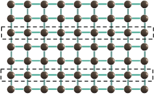
Figure 1: Measurement-based quantum computing as generalization of the one-way model as being considered in this work. Initially, an entangled resource state is available, different from the cluster state, followed by local projective measurements on all individual constituents in the regular not necessarily cubic lattice. In all figures, dark gray circles denote individual physical systems.

We will further see that there is quite some flexibility concerning the computational model itself (addressing Question 2 mentioned in the introduction):

• The new schemes differ from the one-way model in the way the inherent randomness of quantum measurements is dealt with.

• We generalize the well-known concept of by-product operators to encompass any finite group. E.g. we show the existence of computational models, where the by-product operators are elements of the entire single-qubit Clifford group, or the dihedral group.

• We explore schemes where each logical qubit is encoded in several neighboring correlation systems (see Section III for a definition of the term “correlation system”).

• One can find ways to construct schemes in which interactions between logical qubits are controlled by “routing” the qubits towards an “interaction zone” or keeping them away from it.

• In many schemes, we adjust the layout of the measurement pattern dynamically, incorporating information about previous measurement outcomes as we go along. In particular, the expected length of a computation is random (this constitutes no problem, as the probability of exceeding a finite expected length is exponentially small in the excess).

II.1 Universal resource states

What are the properties from which a universal resource state derives its power? After clarifying the terminology, we will argue that an answer to this question – desirable as it may be – faces formidable obstacles.

Quantum computation can come in a variety of different incarnations, as diverse as e.g., the well-known gate-model [32], adiabatic quantum computation [33] or MBQC. All these models turn out to be equivalent in that they can simulate each other efficiently.

For measurement-based schemes, the “hardware” consists of a multi-particle quantum system in an algorithm-independent state and a classical computer. The input is a gate-model description of a quantum computation. In every step of the computation, a local measurement is performed on the quantum state and the result is fed into the classical computer. Based on the outcomes of previous steps, the computer calculates which basis to use for the next measurements and, finally, infers the result of the computation from the measurement outcomes [3]. Having this procedure in mind, we call a quantum state a universal resource for MBQC, if a classical computer assisted by local measurements on this states can efficiently predict the outcome of any quantum computation.

The reader should be aware that another approach has recently been described in the literature. The cluster state has actually a stronger property than the one just used for the definition of universality: it is a universal preparator. This means that one can prepare any given quantum state on a given sub-set of sites of a sufficiently large cluster by means of local measurements. Hence, cluster states could in principle be used for information processing tasks which require a quantum output. Ref. [25] referred to this scenario as CQ-universality – i.e. universality for problems which require a classical input but deliver a quantum output. This observation is the basis of Ref. [24], where a state is called a universal resource if it possesses the strong property of being a universal preparator, or, equivalently, of being CQ-universal.

Clearly, any efficient universal preparator is also a computationally universal resource for MBQC (since one can, in particular, prepare the cluster state). But the converse is not true, as our results show. Indeed, while it proves possible to come up with necessary criteria for a state to be a universal preparator [24], we will argue below that the current limited understanding of quantum computers makes it extremely hard to specify necessary conditions for computational universality.

In order to pinpoint the source of the quantum speedup, we might try to find schemes where more and more work is done by the classical computer, while the employed quantum states become “simpler” (e.g., smaller or less entangled). How far can we push this program without losing universality? The answer is likely to be intractable. Currently, we are not aware of a proof that quantum computation is indeed more powerful than classical methods. Hence, it can presently not be excluded that no assistance from a quantum state is necessary at all.

Observation 1 (Any state may be a universal resource).

If one is unwilling to assume that there is a separation between classical and quantum computation (i.e., BPP $\neq$ BQP), then it is impossible to rule out any state as a universal resource.

It is, however, both common and sensible to assume superiority of quantum computers and we will from now on do so. Observation 1 still serves a purpose: it teaches us that the only known way to rule out universality is to invoke this assumption (this avenue was taken, e.g., in Refs. [34, 16]).

Observation 2 (Efficient classical simulation).

The only currently known method for excluding the possibility that a given quantum state forms a universal resource is to show that any measurement-based scheme utilizing the state can be efficiently simulated by a classical computer.

Thus, the situation presents itself as follows: there is a tiny set of quantum states for which it is possible to prove that any local measurement-based scheme can be efficiently simulated. On the other extreme, there is an even tinier set for which universality is provable. For the vast majority no assessment can be made. Furthermore, given the fact that rigorously establishing the “hardness” of many important problems in computer science turned out to be extremely challenging, it seems unlikely that this situation will change dramatically in the foreseeable future.

We conclude that a search for necessary conditions for universality is likely to remain futile. The converse question, however, can be pursued: it is possible to show that many properties that one might naively assume to be present in any universal resource are, in fact, unnecessary.

III Computational tensor networks

The current section is devoted to an in-depth treatment of a class of states known respectively as valence-bond states, finitely correlated states, matrix product states or projected entangled pairs states, adapted to our purposes of measurement-based quantum computing. This family turns out to be especially well-suited for a description of a computing scheme.

Indeed, any systematic analysis of resources states requires a framework for describing quantum states on extended systems. We briefly compile a list of desiderata, based on which candidate techniques can be assessed.

• The description should be scalable, so that a class of states on systems of arbitrary size can be treated efficiently.

• As quantum states which are naturally described in terms of one-dimensional topologies have been shown to be classically simulable [26, 15, 16], the framework ought to handle two- or higher dimensional topologies naturally.

• The basic operation in measurement-based computation are local measurements. It would be desirable to describe the effect of local measurements in a local manner. Ideally, the class of efficiently describable states should be closed under local measurements.

• The class of describable states should include elements which show features that naturally occur in ground states of quantum many-body systems, such as non-maximal local entropy of entanglement or non-vanishing two-point correlations, etc.

The description of states to be introduced below complies with all of these points.

We will introduce the construction in several steps, starting with one-dimensional matrix product states. The new view on the processing of information is that the matrices appearing in the description of resource states are taken literally, as operators processing quantum information.

III.1 Matrix product states

A matrix product state (MPS) for a chain of $n$ systems of physical dimension $d$ (so $d=2$ for qubits) is specified by

• An auxiliary $D$ dimensional vector space ($D$ being some parameter, describing the amount of correlation between two consecutive blocks of the chain),

• For each system $i$ a set of $d$ $D\times D$-matrices $A_{i}[j],j\in\{0\dots d-1\}$.

• Two $D$-dimensional vectors $\mbox{$|L\rangle$},\mbox{$|R\rangle$}$ representing boundary conditions.

The state vector $|\Psi\rangle$ of the matrix product state is then given explicitly by

$$\mbox{$|\Psi\rangle$}=\sum_{s_{1},\dots,s_{n}=0}^{d-1}\mbox{$\langle R|$}A_{n}[s_{n}]\dots A_{1}[s_{1}]\mbox{$|L\rangle$}\,\,\mbox{$|s_{1},\dots,s_{n}\rangle$}.$$ (2)

From now on we will assume that the matrices are site-independent: $A_{i}[j]=A[j]$, so the MPS is translationally invariant up to the boundary conditions. We take the freedom of disregarding normalization whenever this consistently possible.

Let us spend a minute interpreting Eq. (2). Assume we have measured the first site in the computational basis and obtained the outcome $s_{1}$. One immediately sees that the resulting state vector $|\Psi^{\prime}(s_{1})\rangle$ on the remaining sites is again a MPS, where the left-hand side boundary vector now reads

$$\mbox{$|L^{\prime}(s_{1})\rangle$}=A[s_{1}]\mbox{$|L\rangle$}.$$ (3)

Hence the state of the auxiliary system gets changed according to the measurement outcome. So we find that the correlations between the state of the first site and the rest of the chain are mediated via the auxiliary space, which will thus be referred to as correlation space in the sequel.

In the past, the matrices appearing in the definition of $|\Psi\rangle$ have been treated mainly as a collection of variational parameters, used to parametrize ansatz states for ground states of spin chains [26]. However – and that is the basic insight underlying our view on MBQC – Eq. (3) can also be read as an operator $A[s_{1}]$ acting on some quantum state $|L\rangle$. We will elaborate on this interpretation in Section III.2.

In order to translate Eq. (2) to the setting of 2-D lattices, we need to cast it into the form of a tensor network. Setting $L_{i}=\mbox{$\langle i|L\rangle$}$ and

$$A[s]_{i,j}:=\mbox{$\langle j|$}A\mbox{$|i\rangle$},$$ (4)

we can write Eq. (2) as

$$\langle s_{1},\dots,s_{n}|\Psi\rangle=\sum_{i_{0},\dots,i_{n}}^{D}L_{i_{0}}A[s_{1}]_{i_{0},i_{1}}\dots A[s_{n}]_{i_{n-1},i_{n}}{R^{\dagger}}_{i_{n}}.$$ (5)

While Eq. (5) is awkward enough, the 2-D equivalent is completely unintelligible. To cure this problem, we introduce a graphical notation which enables an intuitive understanding beyond the 1-D case. In the following, tensors will be represented by boxes, indices by edges:

$$L_{r} = \lx@xy@svg{\hbox{\raise 0.0pt\hbox{\kern 6.40279pt\hbox{\ignorespaces\ignorespaces\ignorespaces\hbox{\vtop{\kern 0.0pt\offinterlineskip\halign{\entry@#!@&&\entry@@#!@\cr&\crcr}}}\ignorespaces{{{\hbox{\framed@@{0.0pt}}}}\hbox{\kern-6.40279pt\raise 0.0pt\hbox{\hbox{\kern 3.0pt\raise-3.41666pt\hbox{$\textstyle{L}$}}}}}\ignorespaces\ignorespaces\ignorespaces\ignorespaces{}{\hbox{\lx@xy@droprule}}\ignorespaces{\hbox{\kern 20.62915pt\raise 0.0pt\hbox{\hbox{\kern 0.0pt\raise 0.0pt\hbox{\lx@xy@tip{1}\lx@xy@tip{-1}}}}}}{\hbox{\lx@xy@droprule}}{\hbox{\lx@xy@droprule}}{\hbox{\kern 20.62915pt\raise 0.0pt\hbox{\hbox{\kern 0.0pt\raise 0.0pt\hbox{\hbox{\kern 3.0pt\raise 0.0pt\hbox{$\textstyle{}$}}}}}}}\ignorespaces}}}}\ignorespaces, \textstyle{L} \textstyle{L}$$ (8)

$$A[s]_{l,r} = \lx@xy@svg{\hbox{\raise 0.0pt\hbox{\kern 3.0pt\hbox{\ignorespaces\ignorespaces\ignorespaces\hbox{\vtop{\kern 0.0pt\offinterlineskip\halign{\entry@#!@&&\entry@@#!@\cr&&\crcr}}}\ignorespaces{\hbox{\kern-3.0pt\raise 0.0pt\hbox{\hbox{\kern 0.0pt\raise 0.0pt\hbox{\hbox{\kern 3.0pt\raise 0.0pt\hbox{$\textstyle{\ignorespaces\ignorespaces\ignorespaces\ignorespaces}$}}}}}}}\ignorespaces\ignorespaces\ignorespaces\ignorespaces{}{\hbox{\lx@xy@droprule}}\ignorespaces{\hbox{\kern 17.22636pt\raise 0.0pt\hbox{\hbox{\kern 0.0pt\raise 0.0pt\hbox{\lx@xy@tip{1}\lx@xy@tip{-1}}}}}}{\hbox{\lx@xy@droprule}}{\hbox{\lx@xy@droprule}}{{{\hbox{\framed@@{0.0pt}}}}\hbox{\kern 17.22636pt\raise 0.0pt\hbox{\hbox{\kern 3.0pt\raise-2.5pt\hbox{$\textstyle{A[s]}$}}}}}\ignorespaces\ignorespaces\ignorespaces\ignorespaces{}{\hbox{\lx@xy@droprule}}\ignorespaces{\hbox{\kern 55.1958pt\raise 0.0pt\hbox{\hbox{\kern 0.0pt\raise 0.0pt\hbox{\lx@xy@tip{1}\lx@xy@tip{-1}}}}}}{\hbox{\lx@xy@droprule}}{\hbox{\lx@xy@droprule}}{\hbox{\kern 55.1958pt\raise 0.0pt\hbox{\hbox{\kern 0.0pt\raise 0.0pt\hbox{\hbox{\kern 3.0pt\raise 0.0pt\hbox{$\textstyle{}$}}}}}}}\ignorespaces}}}}\ignorespaces, \textstyle{A[s]} \textstyle{A[s]}$$ (11)

$${R^{\dagger}}_{l} = \lx@xy@svg{\hbox{\raise 0.0pt\hbox{\kern 3.0pt\hbox{\ignorespaces\ignorespaces\ignorespaces\hbox{\vtop{\kern 0.0pt\offinterlineskip\halign{\entry@#!@&&\entry@@#!@\cr&\crcr}}}\ignorespaces{\hbox{\kern-3.0pt\raise 0.0pt\hbox{\hbox{\kern 0.0pt\raise 0.0pt\hbox{\hbox{\kern 3.0pt\raise 0.0pt\hbox{$\textstyle{\ignorespaces\ignorespaces\ignorespaces\ignorespaces}$}}}}}}}\ignorespaces\ignorespaces\ignorespaces\ignorespaces{}{\hbox{\lx@xy@droprule}}\ignorespaces{\hbox{\kern 17.22636pt\raise 0.0pt\hbox{\hbox{\kern 0.0pt\raise 0.0pt\hbox{\lx@xy@tip{1}\lx@xy@tip{-1}}}}}}{\hbox{\lx@xy@droprule}}{\hbox{\lx@xy@droprule}}{{{\hbox{\framed@@{0.0pt}}}}\hbox{\kern 17.22636pt\raise 0.0pt\hbox{\hbox{\kern 3.0pt\raise-4.38889pt\hbox{$\textstyle{R^{\dagger}}$}}}}}\ignorespaces}}}}\ignorespaces\,. \textstyle{R^{\dagger}} \textstyle{R^{\dagger}}$$ (14)

Needless to say, in the equation above, “$l$” is the index leaving the box on the left-hand-side, “$r$” the right-hand-side one. Connected lines designate contractions of the respective indices. Eq. (2) now reads

$$\langle s_{1},\dots,s_{n}|\Psi\rangle=\lx@xy@svg{\hbox{\raise 0.0pt\hbox{\kern 6.40279pt\hbox{\ignorespaces\ignorespaces\ignorespaces\hbox{\vtop{\kern 0.0pt\offinterlineskip\halign{\entry@#!@&&\entry@@#!@\cr&&&&\crcr}}}\ignorespaces{{{\hbox{\framed@@{0.0pt}}}}\hbox{\kern-6.40279pt\raise 0.0pt\hbox{\hbox{\kern 3.0pt\raise-3.41666pt\hbox{$\textstyle{L}$}}}}}\ignorespaces\ignorespaces\ignorespaces\ignorespaces{}{\hbox{\lx@xy@droprule}}\ignorespaces{}{\hbox{\lx@xy@droprule}}{\hbox{\lx@xy@droprule}}{{{\hbox{\framed@@{0.0pt}}}}\hbox{\kern 20.62915pt\raise 0.0pt\hbox{\hbox{\kern 3.0pt\raise-2.5pt\hbox{$\textstyle{A[s_{1}]}$}}}}}\ignorespaces\ignorespaces\ignorespaces\ignorespaces{}{\hbox{\lx@xy@droprule}}\ignorespaces{}{\hbox{\lx@xy@droprule}}{\hbox{\lx@xy@droprule}}{\hbox{\kern 61.3986pt\raise 0.0pt\hbox{\hbox{\kern 0.0pt\raise 0.0pt\hbox{\hbox{\kern 3.0pt\raise 0.0pt\hbox{$\textstyle{\dots\ignorespaces\ignorespaces\ignorespaces\ignorespaces}$}}}}}}}\ignorespaces\ignorespaces\ignorespaces\ignorespaces{}{\hbox{\lx@xy@droprule}}\ignorespaces{}{\hbox{\lx@xy@droprule}}{\hbox{\lx@xy@droprule}}{{{\hbox{\framed@@{0.0pt}}}}\hbox{\kern 89.12497pt\raise 0.0pt\hbox{\hbox{\kern 3.0pt\raise-2.5pt\hbox{$\textstyle{A[s_{n}]}$}}}}}\ignorespaces\ignorespaces\ignorespaces\ignorespaces{}{\hbox{\lx@xy@droprule}}\ignorespaces{}{\hbox{\lx@xy@droprule}}{\hbox{\lx@xy@droprule}}{{{\hbox{\framed@@{0.0pt}}}}\hbox{\kern 130.45573pt\raise 0.0pt\hbox{\hbox{\kern 3.0pt\raise-4.38889pt\hbox{$\textstyle{R^{\dagger}}$}}}}}\ignorespaces}}}}\ignorespaces. \textstyle{L} \textstyle{A[s_{1}]} \textstyle{\dots\ignorespaces\ignorespaces\ignorespaces\ignorespaces} \textstyle{A[s_{n}]} \textstyle{R^{\dagger}} \textstyle{L} \textstyle{A[s_{1}]} \textstyle{\dots\ignorespaces\ignorespaces\ignorespaces\ignorespaces} \textstyle{A[s_{n}]} \textstyle{R^{\dagger}}$$

A single-index tensor can be interpreted as the expansion coefficients of either a “ket” or a “bra”. Sometimes, we will indicate what interpretation we have in mind by placing arrows on the edges: outgoing arrows designating “kets”, incoming arrows “bras”

$$\lx@xy@svg{\hbox{\raise 0.0pt\hbox{\kern 6.40279pt\hbox{\ignorespaces\ignorespaces\ignorespaces\hbox{\vtop{\kern 0.0pt\offinterlineskip\halign{\entry@#!@&&\entry@@#!@\cr&\crcr}}}\ignorespaces{{{\hbox{\framed@@{0.0pt}}}}\hbox{\kern-6.40279pt\raise 0.0pt\hbox{\hbox{\kern 3.0pt\raise-3.41666pt\hbox{$\textstyle{L}$}}}}}\ignorespaces\ignorespaces\ignorespaces\ignorespaces{}{\hbox{\lx@xy@droprule}}\ignorespaces{\hbox{\kern 20.62915pt\raise 0.0pt\hbox{\hbox{\kern 0.0pt\raise 0.0pt\hbox{\lx@xy@tip{1}\lx@xy@tip{-1}}}}}}{\hbox{\lx@xy@droprule}}{\hbox{\lx@xy@droprule}}{\hbox{\kern 20.62915pt\raise 0.0pt\hbox{\hbox{\kern 0.0pt\raise 0.0pt\hbox{\hbox{\kern 3.0pt\raise 0.0pt\hbox{$\textstyle{}$}}}}}}}\ignorespaces}}}}\ignorespaces=\mbox{$|L\rangle$},\quad\lx@xy@svg{\hbox{\raise 0.0pt\hbox{\kern 3.0pt\hbox{\ignorespaces\ignorespaces\ignorespaces\hbox{\vtop{\kern 0.0pt\offinterlineskip\halign{\entry@#!@&&\entry@@#!@\cr&\crcr}}}\ignorespaces{\hbox{\kern-3.0pt\raise 0.0pt\hbox{\hbox{\kern 0.0pt\raise 0.0pt\hbox{\hbox{\kern 3.0pt\raise 0.0pt\hbox{$\textstyle{\ignorespaces\ignorespaces\ignorespaces\ignorespaces}$}}}}}}}\ignorespaces\ignorespaces\ignorespaces\ignorespaces{}{\hbox{\lx@xy@droprule}}\ignorespaces{\hbox{\kern 17.22636pt\raise 0.0pt\hbox{\hbox{\kern 0.0pt\raise 0.0pt\hbox{\lx@xy@tip{1}\lx@xy@tip{-1}}}}}}{\hbox{\lx@xy@droprule}}{\hbox{\lx@xy@droprule}}{{{\hbox{\framed@@{0.0pt}}}}\hbox{\kern 17.22636pt\raise 0.0pt\hbox{\hbox{\kern 3.0pt\raise-4.38889pt\hbox{$\textstyle{R^{\dagger}}$}}}}}\ignorespaces}}}}\ignorespaces=\mbox{$\langle R|$}. \textstyle{L} \textstyle{R^{\dagger}} \textstyle{L} \textstyle{R^{\dagger}}$$ (15)

Tensors with two indices $A_{l,r}$ can naturally be interpreted as operators. In the graphical notation we often want to think of information flowing from the left to the right, in which case $A=\sum_{l,r}A_{l,r}\mbox{$|r\rangle$}_{r}\mbox{$\langle l|$}_{l}$ would be denoted as

$$\lx@xy@svg{\hbox{\raise 0.0pt\hbox{\kern 3.0pt\hbox{\ignorespaces\ignorespaces\ignorespaces\hbox{\vtop{\kern 0.0pt\offinterlineskip\halign{\entry@#!@&&\entry@@#!@\cr&&\crcr}}}\ignorespaces{\hbox{\kern-3.0pt\raise 0.0pt\hbox{\hbox{\kern 0.0pt\raise 0.0pt\hbox{\hbox{\kern 3.0pt\raise 0.0pt\hbox{$\textstyle{\ignorespaces\ignorespaces\ignorespaces\ignorespaces}$}}}}}}}\ignorespaces\ignorespaces\ignorespaces\ignorespaces{}{\hbox{\lx@xy@droprule}}\ignorespaces{\hbox{\kern 17.22636pt\raise 0.0pt\hbox{\hbox{\kern 0.0pt\raise 0.0pt\hbox{\lx@xy@tip{1}\lx@xy@tip{-1}}}}}}{\hbox{\lx@xy@droprule}}{\hbox{\lx@xy@droprule}}{{{\hbox{\framed@@{0.0pt}}}}\hbox{\kern 17.22636pt\raise 0.0pt\hbox{\hbox{\kern 3.0pt\raise-3.41666pt\hbox{$\textstyle{A}$}}}}}\ignorespaces\ignorespaces\ignorespaces\ignorespaces{}{\hbox{\lx@xy@droprule}}\ignorespaces{\hbox{\kern 44.95273pt\raise 0.0pt\hbox{\hbox{\kern 0.0pt\raise 0.0pt\hbox{\lx@xy@tip{1}\lx@xy@tip{-1}}}}}}{\hbox{\lx@xy@droprule}}{\hbox{\lx@xy@droprule}}{\hbox{\kern 44.95273pt\raise 0.0pt\hbox{\hbox{\kern 0.0pt\raise 0.0pt\hbox{\hbox{\kern 3.0pt\raise 0.0pt\hbox{$\textstyle{}$}}}}}}}\ignorespaces}}}}\ignorespaces=A, \textstyle{A} \textstyle{A}$$ (16)

i.e. with the l.h.s. index being associated with a “bra” and the r.h.s one with a “ket”. The following relations exemplify the definition:

$$\langle R|L\rangle = \lx@xy@svg{\hbox{\raise 0.0pt\hbox{\kern 6.40279pt\hbox{\ignorespaces\ignorespaces\ignorespaces\hbox{\vtop{\kern 0.0pt\offinterlineskip\halign{\entry@#!@&&\entry@@#!@\cr&\crcr}}}\ignorespaces{{{\hbox{\framed@@{0.0pt}}}}\hbox{\kern-6.40279pt\raise 0.0pt\hbox{\hbox{\kern 3.0pt\raise-3.41666pt\hbox{$\textstyle{L}$}}}}}\ignorespaces\ignorespaces\ignorespaces\ignorespaces{}{\hbox{\lx@xy@droprule}}\ignorespaces{}{\hbox{\lx@xy@droprule}}{\hbox{\lx@xy@droprule}}{{{\hbox{\framed@@{0.0pt}}}}\hbox{\kern 17.1413pt\raise 0.0pt\hbox{\hbox{\kern 3.0pt\raise-3.41666pt\hbox{$\textstyle{R}$}}}}}\ignorespaces}}}}\ignorespaces\,, \textstyle{L} \textstyle{R} \textstyle{L} \textstyle{R}$$ (19)

$$A\mbox{$|L\rangle$} = \lx@xy@svg{\hbox{\raise 0.0pt\hbox{\kern 6.40279pt\hbox{\ignorespaces\ignorespaces\ignorespaces\hbox{\vtop{\kern 0.0pt\offinterlineskip\halign{\entry@#!@&&\entry@@#!@\cr&&\crcr}}}\ignorespaces{{{\hbox{\framed@@{0.0pt}}}}\hbox{\kern-6.40279pt\raise 0.0pt\hbox{\hbox{\kern 3.0pt\raise-3.41666pt\hbox{$\textstyle{L}$}}}}}\ignorespaces\ignorespaces\ignorespaces\ignorespaces{}{\hbox{\lx@xy@droprule}}\ignorespaces{}{\hbox{\lx@xy@droprule}}{\hbox{\lx@xy@droprule}}{{{\hbox{\framed@@{0.0pt}}}}\hbox{\kern 20.62915pt\raise 0.0pt\hbox{\hbox{\kern 3.0pt\raise-3.41666pt\hbox{$\textstyle{A}$}}}}}\ignorespaces\ignorespaces\ignorespaces\ignorespaces{}{\hbox{\lx@xy@droprule}}\ignorespaces{\hbox{\kern 48.35551pt\raise 0.0pt\hbox{\hbox{\kern 0.0pt\raise 0.0pt\hbox{\lx@xy@tip{1}\lx@xy@tip{-1}}}}}}{\hbox{\lx@xy@droprule}}{\hbox{\lx@xy@droprule}}{\hbox{\kern 48.35551pt\raise 0.0pt\hbox{\hbox{\kern 0.0pt\raise 0.0pt\hbox{\hbox{\kern 3.0pt\raise 0.0pt\hbox{$\textstyle{}$}}}}}}}\ignorespaces}}}}\ignorespaces, \textstyle{L} \textstyle{A} \textstyle{L} \textstyle{A}$$ (22)

$$AB = \lx@xy@svg{\hbox{\raise 0.0pt\hbox{\kern 3.0pt\hbox{\ignorespaces\ignorespaces\ignorespaces\hbox{\vtop{\kern 0.0pt\offinterlineskip\halign{\entry@#!@&&\entry@@#!@\cr&&&\crcr}}}\ignorespaces{\hbox{\kern-3.0pt\raise 0.0pt\hbox{\hbox{\kern 0.0pt\raise 0.0pt\hbox{\hbox{\kern 3.0pt\raise 0.0pt\hbox{$\textstyle{\ignorespaces\ignorespaces\ignorespaces\ignorespaces}$}}}}}}}\ignorespaces\ignorespaces\ignorespaces\ignorespaces{}{\hbox{\lx@xy@droprule}}\ignorespaces{\hbox{\kern 17.22636pt\raise 0.0pt\hbox{\hbox{\kern 0.0pt\raise 0.0pt\hbox{\lx@xy@tip{1}\lx@xy@tip{-1}}}}}}{\hbox{\lx@xy@droprule}}{\hbox{\lx@xy@droprule}}{{{\hbox{\framed@@{0.0pt}}}}\hbox{\kern 17.22636pt\raise 0.0pt\hbox{\hbox{\kern 3.0pt\raise-3.41666pt\hbox{$\textstyle{B}$}}}}}\ignorespaces\ignorespaces\ignorespaces\ignorespaces{}{\hbox{\lx@xy@droprule}}\ignorespaces{}{\hbox{\lx@xy@droprule}}{\hbox{\lx@xy@droprule}}{{{\hbox{\framed@@{0.0pt}}}}\hbox{\kern 45.53952pt\raise 0.0pt\hbox{\hbox{\kern 3.0pt\raise-3.41666pt\hbox{$\textstyle{A}$}}}}}\ignorespaces\ignorespaces\ignorespaces\ignorespaces{}{\hbox{\lx@xy@droprule}}\ignorespaces{\hbox{\kern 73.26588pt\raise 0.0pt\hbox{\hbox{\kern 0.0pt\raise 0.0pt\hbox{\lx@xy@tip{1}\lx@xy@tip{-1}}}}}}{\hbox{\lx@xy@droprule}}{\hbox{\lx@xy@droprule}}{\hbox{\kern 73.26588pt\raise 0.0pt\hbox{\hbox{\kern 0.0pt\raise 0.0pt\hbox{\hbox{\kern 3.0pt\raise 0.0pt\hbox{$\textstyle{}$}}}}}}}\ignorespaces}}}}\ignorespaces, \textstyle{B} \textstyle{A} \textstyle{B} \textstyle{A}$$ (25)

$$\mbox{tr}(AB) = \lx@xy@svg{\hbox{\raise 0.0pt\hbox{\kern 51.24612pt\hbox{{\hbox{\kern-51.24612pt\raise 0.0pt\hbox{\hbox{\kern 0.0pt\raise 7.26791pt\lx@xy@svgnested{\hbox{\raise 0.0pt\hbox{\kern 3.0pt\hbox{\ignorespaces\ignorespaces\ignorespaces\hbox{\vtop{\kern 0.0pt\offinterlineskip\halign{\entry@#!@&&\entry@@#!@\cr&&&&\\&&&&\crcr}}}\ignorespaces{\hbox{\kern-3.0pt\raise 0.0pt\hbox{\hbox{\kern 0.0pt\raise 0.0pt\hbox{\hbox{\kern 3.0pt\raise 0.0pt\hbox{$\textstyle{}$}}}}}}}{{{\hbox{\framed@@{0.0pt}}}}\hbox{\kern 17.22636pt\raise 0.0pt\hbox{\hbox{\kern 3.0pt\raise-3.41666pt\hbox{$\textstyle{B}$}}}}}\ignorespaces\ignorespaces\ignorespaces\ignorespaces{}{\hbox{\lx@xy@droprule}}\ignorespaces{}{\hbox{\lx@xy@droprule}}{\hbox{\lx@xy@droprule}}{{{\hbox{\framed@@{0.0pt}}}}\hbox{\kern 45.53952pt\raise 0.0pt\hbox{\hbox{\kern 3.0pt\raise-3.41666pt\hbox{$\textstyle{A}$}}}}}\ignorespaces\ignorespaces{\hbox{\kern 68.26588pt\raise-3.99414pt\hbox{\hbox{\kern 0.0pt\raise 0.0pt\hbox{\cirbuild@}}}}}\ignorespaces\ignorespaces\ignorespaces{}{\hbox{\lx@xy@droprule}}{\hbox{\lx@xy@droprule}}\ignorespaces{\hbox{\kern 68.2678pt\raise-13.95247pt\hbox{\hbox{\kern 0.0pt\raise 0.0pt\hbox{\cirbuild@}}}}}\ignorespaces\ignorespaces{\hbox{\lx@xy@droprule}}\ignorespaces{\hbox{\kern 0.0pt\raise-13.95833pt\hbox{\hbox{\kern 0.0pt\raise 0.0pt\hbox{\cirbuild@}}}}}\ignorespaces\ignorespaces{\hbox{\lx@xy@droprule}}\ignorespaces{\hbox{\kern 0.0012pt\raise-4.0pt\hbox{\hbox{\kern 0.0pt\raise 0.0pt\hbox{\cirbuild@}}}}}\ignorespaces\ignorespaces{\hbox{\lx@xy@droprule}}\ignorespaces\ignorespaces\ignorespaces{}{\hbox{\lx@xy@droprule}}{\hbox{\lx@xy@droprule}}{\hbox{\kern 73.26588pt\raise 0.0pt\hbox{\hbox{\kern 0.0pt\raise 0.0pt\hbox{\hbox{\kern 3.0pt\raise 0.0pt\hbox{$\textstyle{}$}}}}}}}{\hbox{\kern 93.49225pt\raise 0.0pt\hbox{\hbox{\kern 0.0pt\raise 0.0pt\hbox{\hbox{\kern 3.0pt\raise 0.0pt\hbox{$\textstyle{}$}}}}}}}{\hbox{\kern-3.0pt\raise-17.95247pt\hbox{\hbox{\kern 0.0pt\raise 0.0pt\hbox{\hbox{\kern 3.0pt\raise 0.0pt\hbox{$\textstyle{}$}}}}}}}{\hbox{\kern 21.26976pt\raise-17.95247pt\hbox{\hbox{\kern 0.0pt\raise 0.0pt\hbox{\hbox{\kern 3.0pt\raise 0.0pt\hbox{$\textstyle{}$}}}}}}}{\hbox{\kern 49.28952pt\raise-17.95247pt\hbox{\hbox{\kern 0.0pt\raise 0.0pt\hbox{\hbox{\kern 3.0pt\raise 0.0pt\hbox{$\textstyle{}$}}}}}}}{\hbox{\kern 73.26588pt\raise-17.95247pt\hbox{\hbox{\kern 0.0pt\raise 0.0pt\hbox{\hbox{\kern 3.0pt\raise 0.0pt\hbox{$\textstyle{}$}}}}}}}{\hbox{\kern 93.49225pt\raise-17.95247pt\hbox{\hbox{\kern 0.0pt\raise 0.0pt\hbox{\hbox{\kern 3.0pt\raise 0.0pt\hbox{$\textstyle{}$}}}}}}}\ignorespaces\ignorespaces}}}}}}}}}}}}. \textstyle{B} \textstyle{A} \textstyle{B} \textstyle{A}$$ (30)

The formula for the expansion coefficients of a matrix product state finally becomes

$$\langle s_{1},\dots,s_{n}|\Psi\rangle=\ \lx@xy@svg{\hbox{\raise 0.0pt\hbox{\kern 6.40279pt\hbox{\ignorespaces\ignorespaces\ignorespaces\hbox{\vtop{\kern 0.0pt\offinterlineskip\halign{\entry@#!@&&\entry@@#!@\cr&&&&\crcr}}}\ignorespaces{{{\hbox{\framed@@{0.0pt}}}}\hbox{\kern-6.40279pt\raise 0.0pt\hbox{\hbox{\kern 3.0pt\raise-3.41666pt\hbox{$\textstyle{L}$}}}}}\ignorespaces\ignorespaces\ignorespaces\ignorespaces{}{\hbox{\lx@xy@droprule}}\ignorespaces{}{\hbox{\lx@xy@droprule}}{\hbox{\lx@xy@droprule}}{{{\hbox{\framed@@{0.0pt}}}}\hbox{\kern 20.62915pt\raise 0.0pt\hbox{\hbox{\kern 3.0pt\raise-2.5pt\hbox{$\textstyle{A[s_{1}]}$}}}}}\ignorespaces\ignorespaces\ignorespaces\ignorespaces{}{\hbox{\lx@xy@droprule}}\ignorespaces{}{\hbox{\lx@xy@droprule}}{\hbox{\lx@xy@droprule}}{\hbox{\kern 61.3986pt\raise 0.0pt\hbox{\hbox{\kern 0.0pt\raise 0.0pt\hbox{\hbox{\kern 3.0pt\raise 0.0pt\hbox{$\textstyle{\dots\ignorespaces\ignorespaces\ignorespaces\ignorespaces}$}}}}}}}\ignorespaces\ignorespaces\ignorespaces\ignorespaces{}{\hbox{\lx@xy@droprule}}\ignorespaces{}{\hbox{\lx@xy@droprule}}{\hbox{\lx@xy@droprule}}{{{\hbox{\framed@@{0.0pt}}}}\hbox{\kern 89.12497pt\raise 0.0pt\hbox{\hbox{\kern 3.0pt\raise-2.5pt\hbox{$\textstyle{A[s_{n}]}$}}}}}\ignorespaces\ignorespaces\ignorespaces\ignorespaces{}{\hbox{\lx@xy@droprule}}\ignorespaces{}{\hbox{\lx@xy@droprule}}{\hbox{\lx@xy@droprule}}{{{\hbox{\framed@@{0.0pt}}}}\hbox{\kern 130.45573pt\raise 0.0pt\hbox{\hbox{\kern 3.0pt\raise-4.38889pt\hbox{$\textstyle{R^{\dagger}}$}}}}}\ignorespaces}}}}\ignorespaces\,. \textstyle{L} \textstyle{A[s_{1}]} \textstyle{\dots\ignorespaces\ignorespaces\ignorespaces\ignorespaces} \textstyle{A[s_{n}]} \textstyle{R^{\dagger}} \textstyle{L} \textstyle{A[s_{1}]} \textstyle{\dots\ignorespaces\ignorespaces\ignorespaces\ignorespaces} \textstyle{A[s_{n}]} \textstyle{R^{\dagger}}$$

This formula suggest a more “dynamic” interpretation of MPS: the l.h.s. boundary conditions $|L\rangle$ specify an initial state of the correlation system, which is acted on by the matrices of the MPS representation. The next paragraph is going to elaborate on this point.

III.2 Quantum computing in correlation systems

We return to the discussion of the properties of matrix product states. Above, it has been shown how to compute the overlap of $|\Psi\rangle$ with an element of the computational basis (c.f. Eq. (5)). The next step is to generalize this to any local projection operator. Indeed, if $|\phi\rangle$ is a general state vector in $\mathbb{C}^{2}$, we abbreviate

$$\mbox{$\langle\phi|0\rangle$}\,A[0]+\mbox{$\langle\phi|1\rangle$}\,A[1]=:A[\phi].$$ (31)

One then easily derives the following, central formula

$$\big{(}\bigotimes_{i}^{n}\mbox{$\langle\phi_{i}|$}\big{)}\mbox{$|\Psi\rangle$}=\lx@xy@svg{\hbox{\raise 0.0pt\hbox{\kern 6.40279pt\hbox{\ignorespaces\ignorespaces\ignorespaces\hbox{\vtop{\kern 0.0pt\offinterlineskip\halign{\entry@#!@&&\entry@@#!@\cr&&&&\crcr}}}\ignorespaces{{{\hbox{\framed@@{0.0pt}}}}\hbox{\kern-6.40279pt\raise 0.0pt\hbox{\hbox{\kern 3.0pt\raise-3.41666pt\hbox{$\textstyle{L}$}}}}}\ignorespaces\ignorespaces\ignorespaces\ignorespaces{}{\hbox{\lx@xy@droprule}}\ignorespaces{}{\hbox{\lx@xy@droprule}}{\hbox{\lx@xy@droprule}}{{{\hbox{\framed@@{0.0pt}}}}\hbox{\kern 9.24805pt\raise 0.0pt\hbox{\hbox{\kern 3.0pt\raise-2.5pt\hbox{$\textstyle{A[\phi_{1}]}$}}}}}\ignorespaces\ignorespaces\ignorespaces\ignorespaces{}{\hbox{\lx@xy@droprule}}\ignorespaces{}{\hbox{\lx@xy@droprule}}{\hbox{\lx@xy@droprule}}{\hbox{\kern 39.90724pt\raise 0.0pt\hbox{\hbox{\kern 0.0pt\raise 0.0pt\hbox{\hbox{\kern 3.0pt\raise 0.0pt\hbox{$\textstyle{\dots\ignorespaces\ignorespaces\ignorespaces\ignorespaces}$}}}}}}}\ignorespaces\ignorespaces\ignorespaces\ignorespaces{}{\hbox{\lx@xy@droprule}}\ignorespaces{}{\hbox{\lx@xy@droprule}}{\hbox{\lx@xy@droprule}}{{{\hbox{\framed@@{0.0pt}}}}\hbox{\kern 56.2525pt\raise 0.0pt\hbox{\hbox{\kern 3.0pt\raise-2.5pt\hbox{$\textstyle{A[\phi_{n}]}$}}}}}\ignorespaces\ignorespaces\ignorespaces\ignorespaces{}{\hbox{\lx@xy@droprule}}\ignorespaces{}{\hbox{\lx@xy@droprule}}{\hbox{\lx@xy@droprule}}{{{\hbox{\framed@@{0.0pt}}}}\hbox{\kern 87.473pt\raise 0.0pt\hbox{\hbox{\kern 3.0pt\raise-3.41666pt\hbox{$\textstyle{R}$}}}}}\ignorespaces}}}}\ignorespaces\,\,. \textstyle{L} \textstyle{A[\phi_{1}]} \textstyle{\dots\ignorespaces\ignorespaces\ignorespaces\ignorespaces} \textstyle{A[\phi_{n}]} \textstyle{R} \textstyle{L} \textstyle{A[\phi_{1}]} \textstyle{\dots\ignorespaces\ignorespaces\ignorespaces\ignorespaces} \textstyle{A[\phi_{n}]} \textstyle{R}$$ (32)

Now suppose we measure local observables on $|\Psi\rangle$ and obtain results corresponding to the eigenvector $|\phi_{i}\rangle$ at the $i$-th site. Eq. (32) allows us to re-interpret this process as follows. Initially, the $D$-dimensional correlation system is prepared in the state $|L\rangle$. The result $|\phi_{1}\rangle$ at the first site induces the evolution

$$\mbox{$|L\rangle$}\mapsto A[\phi_{1}]\mbox{$|L\rangle$}.$$ (33)

From this point of view, a sequence of measurements on $|\Psi\rangle$ is tantamount to a processing of the correlation system’s state by the operations $A[\phi_{i}]$. An appealing perspective on MBC suggests itself:

Observation 3 (Role of correlation space).

Measurement-based computing takes place in correlation space. The gates acting on the correlation systems are determined by local measurements. Intuitively, “quantum correlations” are the source of a resource’s computational potency. The strength of this framework lies in the fact that it assigns a concrete mathematical object to these correlations.

Indeed, it will turn out that MBQC can be understood completely using this interpretation.

III.3 Example: The 1-D cluster state

To illustrate the abstract definitions made above, we will discuss the linear cluster state vector $|Cl_{n}\rangle$ in this section. It is both one of the simplest and certainly the most important MPS in the context of MBQC.

What is the tensor network representation of $|Cl_{n}\rangle$? Recall that the cluster state can be generated by preparing $n$ sites in the state vector $\mbox{$|+\rangle$}:=\mbox{$|0\rangle$}+\mbox{$|1\rangle$}$ and subsequently applying the controlled-$Z$ operation

$$CZ=|0,0\rangle\langle 0,0|+|0,1\rangle\langle 0,1|+|1,0\rangle\langle 1,0|-|1,1\rangle\langle 1,1|$$ (34)

between any two nearest neighbors. Effectively, $CZ$ introduces a $\pi$-phase whenever two consecutive systems are in the $|1\rangle$-state. Hence its expansion coefficients in the computational basis are given by

$$\mbox{$\langle s_{1},\dots,s_{n}|Cl_{n}\rangle$}=2^{-n/2}(-1)^{p},$$ (35)

where $p$ denotes the number of sites $i$ such that $s_{i}=s_{i+1}=1$.

This observation makes it simple to derive the tensors of the MPS representation. We need a $D=2$-dimensional correlation system, which – loosely speaking – will convey the information about the state $s_{i}$ of the $i$-th site to site $i+1$. Define the matrices $A[0/1]$ by

(38)

(41)

The intuition behind this choice is as follows. By the elementary relations

$$\mbox{$\langle+|0\rangle$}=\mbox{$\langle+|1\rangle$}=\mbox{$\langle-|0\rangle$}=2^{-1/2},\qquad\mbox{$\langle-|1\rangle$}=-2^{-1/2},$$ (42)

the contraction in the middle of

(43)

will yield a sign of ”$-1$” exactly if $s_{1}=s_{2}=1$. Indeed, setting the boundary vectors to $\mbox{$|L\rangle$}=\mbox{$|0\rangle$},\mbox{$|R\rangle$}=\mbox{$|+\rangle$}$ one checks easily that

$$\mbox{$\langle R|$}A[s_{n}]\dots A[s_{1}]\mbox{$|L\rangle$}=2^{-n/2}(-1)^{p},$$ (44)

which is exactly the value required by Eq. (35).

Below, we will interpret the correlation system of a 1-D chain as a single logical quantum system. For this interpretation to be viable, we must check that the following basic operations can be performed deterministically by local measurements: i) prepare the correlation system in a known initial state, ii) transport that state along the chain (possibly subject to known unitary transformations) and iii) read out the final state.

To set the state of the correlation system to a definitive value, we measure some site – say the $i$-th – in the $Z$-eigenbasis. Throughout this work, we will choose the notation $X$, $Y$, and $Z$ for the Pauli operators. Denote the measurement outcome by $z\in\{0,1\}$. In case of $z=0$, Eq. (38) tells us that the state of the correlation system to the right of the $i$-th site will be $|+\rangle$ (up to an unimportant phase). Likewise, a $z=1$ outcome prepares the correlation system in $|-\rangle$, according to Eq. (41). It follows that we can use $Z$-measurements for preparation. How to cope with the intrinsic randomness of quantum measurements will concern us later.

Secondly, consider the operators

(51)

$$\propto \mbox{$|+\rangle$}\mbox{$\langle 0|$}+\mbox{$|-\rangle$}\mbox{$\langle 1|$}=H,$$ (52)

(55)

where $H$ is the Hadamard-gate. We see immediately that measurements in the $X$-eigenbasis give rise to a unitary evolution on the correlation space. Similarly, one can show that one can generate arbitrary local unitaries by appropriate measurements in the $Y$-$Z$ plane.

Below, we will frequently be confronted with a situation like the one presented in Eqs. (52,55), where the correlation system evolves in one of two possibilities, dependent on the outcome of a measurement. It will be convenient to introduce a compact notation that encompasses both cases in a single equation. So Eqs. (52,55) will be represented as

$$\lx@xy@svg{\hbox{\raise 0.0pt\hbox{\kern 3.0pt\hbox{\ignorespaces\ignorespaces\ignorespaces\hbox{\vtop{\kern 0.0pt\offinterlineskip\halign{\entry@#!@&&\entry@@#!@\cr&&\crcr}}}\ignorespaces{\hbox{\kern-3.0pt\raise 0.0pt\hbox{\hbox{\kern 0.0pt\raise 0.0pt\hbox{\hbox{\kern 3.0pt\raise 0.0pt\hbox{$\textstyle{\ignorespaces\ignorespaces\ignorespaces\ignorespaces}$}}}}}}}\ignorespaces\ignorespaces\ignorespaces\ignorespaces{}{\hbox{\lx@xy@droprule}}\ignorespaces{\hbox{\kern 17.22636pt\raise 0.0pt\hbox{\hbox{\kern 0.0pt\raise 0.0pt\hbox{\lx@xy@tip{1}\lx@xy@tip{-1}}}}}}{\hbox{\lx@xy@droprule}}{\hbox{\lx@xy@droprule}}{{{\hbox{\framed@@{0.0pt}}}}\hbox{\kern 17.22636pt\raise 0.0pt\hbox{\hbox{\kern 3.0pt\raise-2.5pt\hbox{$\textstyle{A[X]}$}}}}}\ignorespaces\ignorespaces\ignorespaces\ignorespaces{}{\hbox{\lx@xy@droprule}}\ignorespaces{\hbox{\kern 59.57773pt\raise 0.0pt\hbox{\hbox{\kern 0.0pt\raise 0.0pt\hbox{\lx@xy@tip{1}\lx@xy@tip{-1}}}}}}{\hbox{\lx@xy@droprule}}{\hbox{\lx@xy@droprule}}{\hbox{\kern 59.57773pt\raise 0.0pt\hbox{\hbox{\kern 0.0pt\raise 0.0pt\hbox{\hbox{\kern 3.0pt\raise 0.0pt\hbox{$\textstyle{}$}}}}}}}\ignorespaces}}}}\ignorespaces=HZ^{x}. \textstyle{A[X]} \textstyle{A[X]}$$ (56)

Here $x=0$ corresponds to the outcome $|+\rangle$ in an $X$-measurement, whereas $x=1$ corresponds to the outcome $|-\rangle$. In general, a physical observable given as an argument to a tensor corresponds to a measurement in the observable’s eigenbasis. The measurement outcome is assigned to a suitable variable as in the above example.

Lastly, we must show how to physically read out the state of the purely logical correlation system. It turns out that measuring the $i+1$-th physical system in the $Z$-eigenbasis corresponds to a $Z$-measurement of the state of the correlation system just after site $i$. Indeed, suppose we have measured the first $i$ systems and obtained results corresponding to the local projection operator $\mbox{$|\phi_{1}\rangle$}\otimes\dots\otimes\mbox{$|\phi_{i}\rangle$}$. Further assume that as a result of these measurements the correlation system is in the state $|0\rangle$:

$$\lx@xy@svg{\hbox{\raise 0.0pt\hbox{\kern 6.40279pt\hbox{\ignorespaces\ignorespaces\ignorespaces\hbox{\vtop{\kern 0.0pt\offinterlineskip\halign{\entry@#!@&&\entry@@#!@\cr&&&&\crcr}}}\ignorespaces{{{\hbox{\framed@@{0.0pt}}}}\hbox{\kern-6.40279pt\raise 0.0pt\hbox{\hbox{\kern 3.0pt\raise-3.41666pt\hbox{$\textstyle{L}$}}}}}\ignorespaces\ignorespaces\ignorespaces\ignorespaces{}{\hbox{\lx@xy@droprule}}\ignorespaces{}{\hbox{\lx@xy@droprule}}{\hbox{\lx@xy@droprule}}{{{\hbox{\framed@@{0.0pt}}}}\hbox{\kern 9.24805pt\raise 0.0pt\hbox{\hbox{\kern 3.0pt\raise-2.5pt\hbox{$\textstyle{A[\phi_{1}]}$}}}}}\ignorespaces\ignorespaces\ignorespaces\ignorespaces{}{\hbox{\lx@xy@droprule}}\ignorespaces{}{\hbox{\lx@xy@droprule}}{\hbox{\lx@xy@droprule}}{\hbox{\kern 39.90724pt\raise 0.0pt\hbox{\hbox{\kern 0.0pt\raise 0.0pt\hbox{\hbox{\kern 3.0pt\raise 0.0pt\hbox{$\textstyle{\dots\ignorespaces\ignorespaces\ignorespaces\ignorespaces}$}}}}}}}\ignorespaces\ignorespaces\ignorespaces\ignorespaces{}{\hbox{\lx@xy@droprule}}\ignorespaces{}{\hbox{\lx@xy@droprule}}{\hbox{\lx@xy@droprule}}{{{\hbox{\framed@@{0.0pt}}}}\hbox{\kern 56.2525pt\raise 0.0pt\hbox{\hbox{\kern 3.0pt\raise-2.5pt\hbox{$\textstyle{A[\phi_{i}]}$}}}}}\ignorespaces\ignorespaces\ignorespaces\ignorespaces{}{\hbox{\lx@xy@droprule}}\ignorespaces{\hbox{\kern 86.04097pt\raise 0.0pt\hbox{\hbox{\kern 0.0pt\raise 0.0pt\hbox{\lx@xy@tip{1}\lx@xy@tip{-1}}}}}}{\hbox{\lx@xy@droprule}}{\hbox{\lx@xy@droprule}}{\hbox{\kern 86.04097pt\raise 0.0pt\hbox{\hbox{\kern 0.0pt\raise 0.0pt\hbox{\hbox{\kern 3.0pt\raise 0.0pt\hbox{$\textstyle{}$}}}}}}}\ignorespaces}}}}\ignorespaces=\mbox{$|0\rangle$}. \textstyle{L} \textstyle{A[\phi_{1}]} \textstyle{\dots\ignorespaces\ignorespaces\ignorespaces\ignorespaces} \textstyle{A[\phi_{i}]} \textstyle{L} \textstyle{A[\phi_{1}]} \textstyle{\dots\ignorespaces\ignorespaces\ignorespaces\ignorespaces} \textstyle{A[\phi_{i}]}$$ (57)

Using Eq. (41) we have that

$$\propto \mbox{$|+\rangle$}\mbox{$\langle 1|0\rangle$}=0.$$

But then it follows from Eq. (32) that the probability of obtaining the result $1$ for a $Z$-measurement on site $i+1$ is equal to zero. In other words: if the correlation system is in the state $|0\rangle$ after the $i$-th site, then the $i+1$-th physical site must also be in the state $|0\rangle$. An analogous argument for the $|1\rangle$-case completes the description of the read-out scheme.

III.4 2-D lattices

The graphical notation greatly facilitates the passage to 2-D lattices. Here, the tensors $A[s]$ have four indices $A[s]_{l,r,u,d}$, which will be contracted with the indices of the left, right, upper and lower neighboring tensors respectively. After choosing a set of boundary conditions $\mbox{$|L\rangle$},\mbox{$|R\rangle$},\mbox{$|U\rangle$},\mbox{$|D\rangle$}\in\mathbb{C}^{D}$, the expansion coefficients of the state vector $|\Psi\rangle$ are computed as illustrated in the following example on a $2\times 2$-lattice:

$$\mbox{$\langle s_{1,1},\dots,s_{2,2}|\Psi\rangle$}=\lx@xy@svg{\hbox{\raise 0.0pt\hbox{\kern 56.9402pt\hbox{{\hbox{\kern-56.9402pt\raise 0.0pt\hbox{\hbox{\kern 0.0pt\raise 35.61368pt\lx@xy@svgnested{\hbox{\raise 0.0pt\hbox{\kern 6.40279pt\hbox{\ignorespaces\ignorespaces\ignorespaces\hbox{\vtop{\kern 0.0pt\offinterlineskip\halign{\entry@#!@&&\entry@@#!@\cr&&\\&&&\\&&&\\&&\crcr}}}\ignorespaces{\hbox{\kern-3.0pt\raise 0.0pt\hbox{\hbox{\kern 0.0pt\raise 0.0pt\hbox{\hbox{\kern 3.0pt\raise 0.0pt\hbox{$\textstyle{}$}}}}}}}{{{\hbox{\framed@@{0.0pt}}}}\hbox{\kern 23.4289pt\raise 0.0pt\hbox{\hbox{\kern 3.0pt\raise-3.41666pt\hbox{$\textstyle{U}$}}}}}{{{\hbox{\framed@@{0.0pt}}}}\hbox{\kern 62.86333pt\raise 0.0pt\hbox{\hbox{\kern 3.0pt\raise-3.41666pt\hbox{$\textstyle{U}$}}}}}{{{\hbox{\framed@@{0.0pt}}}}\hbox{\kern-6.40279pt\raise-23.14912pt\hbox{\hbox{\kern 3.0pt\raise-3.41666pt\hbox{$\textstyle{L}$}}}}}\ignorespaces\ignorespaces\ignorespaces\ignorespaces{}{\hbox{\lx@xy@droprule}}\ignorespaces{}{\hbox{\lx@xy@droprule}}{\hbox{\lx@xy@droprule}}{{{\hbox{\framed@@{0.0pt}}}}\hbox{\kern 14.9386pt\raise-23.14912pt\hbox{\hbox{\kern 3.0pt\raise-2.30334pt\hbox{$\textstyle{A[s_{1,1}]}$}}}}}\ignorespaces\ignorespaces\ignorespaces\ignorespaces{}{\hbox{\lx@xy@droprule}}\ignorespaces{}{\hbox{\lx@xy@droprule}}{\hbox{\lx@xy@droprule}}\ignorespaces\ignorespaces\ignorespaces\ignorespaces{}{\hbox{\lx@xy@droprule}}\ignorespaces{}{\hbox{\lx@xy@droprule}}{\hbox{\lx@xy@droprule}}{{{\hbox{\framed@@{0.0pt}}}}\hbox{\kern 54.37303pt\raise-23.14912pt\hbox{\hbox{\kern 3.0pt\raise-2.30334pt\hbox{$\textstyle{A[s_{2,1}]}$}}}}}\ignorespaces\ignorespaces\ignorespaces\ignorespaces{}{\hbox{\lx@xy@droprule}}\ignorespaces{}{\hbox{\lx@xy@droprule}}{\hbox{\lx@xy@droprule}}\ignorespaces\ignorespaces\ignorespaces\ignorespaces{}{\hbox{\lx@xy@droprule}}\ignorespaces{}{\hbox{\lx@xy@droprule}}{\hbox{\lx@xy@droprule}}{{{\hbox{\framed@@{0.0pt}}}}\hbox{\kern 93.80746pt\raise-23.14912pt\hbox{\hbox{\kern 3.0pt\raise-3.41666pt\hbox{$\textstyle{R}$}}}}}{{{\hbox{\framed@@{0.0pt}}}}\hbox{\kern-6.40279pt\raise-48.07825pt\hbox{\hbox{\kern 3.0pt\raise-3.41666pt\hbox{$\textstyle{L}$}}}}}\ignorespaces\ignorespaces\ignorespaces\ignorespaces{}{\hbox{\lx@xy@droprule}}\ignorespaces{}{\hbox{\lx@xy@droprule}}{\hbox{\lx@xy@droprule}}{{{\hbox{\framed@@{0.0pt}}}}\hbox{\kern 14.9386pt\raise-48.07825pt\hbox{\hbox{\kern 3.0pt\raise-2.30334pt\hbox{$\textstyle{A[s_{1,2}]}$}}}}}\ignorespaces\ignorespaces\ignorespaces\ignorespaces{}{\hbox{\lx@xy@droprule}}\ignorespaces{}{\hbox{\lx@xy@droprule}}{\hbox{\lx@xy@droprule}}\ignorespaces\ignorespaces\ignorespaces\ignorespaces{}{\hbox{\lx@xy@droprule}}\ignorespaces{}{\hbox{\lx@xy@droprule}}{\hbox{\lx@xy@droprule}}{{{\hbox{\framed@@{0.0pt}}}}\hbox{\kern 54.37303pt\raise-48.07825pt\hbox{\hbox{\kern 3.0pt\raise-2.30334pt\hbox{$\textstyle{A[s_{2,2}]}$}}}}}\ignorespaces\ignorespaces\ignorespaces\ignorespaces{}{\hbox{\lx@xy@droprule}}\ignorespaces{}{\hbox{\lx@xy@droprule}}{\hbox{\lx@xy@droprule}}\ignorespaces\ignorespaces\ignorespaces\ignorespaces{}{\hbox{\lx@xy@droprule}}\ignorespaces{}{\hbox{\lx@xy@droprule}}{\hbox{\lx@xy@droprule}}{{{\hbox{\framed@@{0.0pt}}}}\hbox{\kern 93.80746pt\raise-48.07825pt\hbox{\hbox{\kern 3.0pt\raise-3.41666pt\hbox{$\textstyle{R}$}}}}}{\hbox{\kern-3.0pt\raise-71.22737pt\hbox{\hbox{\kern 0.0pt\raise 0.0pt\hbox{\hbox{\kern 3.0pt\raise 0.0pt\hbox{$\textstyle{}$}}}}}}}{{{\hbox{\framed@@{0.0pt}}}}\hbox{\kern 23.10944pt\raise-71.22737pt\hbox{\hbox{\kern 3.0pt\raise-3.41666pt\hbox{$\textstyle{D}$}}}}}\ignorespaces\ignorespaces\ignorespaces\ignorespaces{}{\hbox{\lx@xy@droprule}}\ignorespaces{}{\hbox{\lx@xy@droprule}}{\hbox{\lx@xy@droprule}}{{{\hbox{\framed@@{0.0pt}}}}\hbox{\kern 62.54387pt\raise-71.22737pt\hbox{\hbox{\kern 3.0pt\raise-3.41666pt\hbox{$\textstyle{D}$}}}}}\ignorespaces\ignorespaces\ignorespaces\ignorespaces{}{\hbox{\lx@xy@droprule}}\ignorespaces{}{\hbox{\lx@xy@droprule}}{\hbox{\lx@xy@droprule}}\ignorespaces\ignorespaces}}}}}}}}}}}}. \textstyle{U} \textstyle{U} \textstyle{L} \textstyle{A[s_{1,1}]} \textstyle{A[s_{2,1}]} \textstyle{R} \textstyle{L} \textstyle{A[s_{1,2}]} \textstyle{A[s_{2,2}]} \textstyle{R} \textstyle{D} \textstyle{D} \textstyle{U} \textstyle{U} \textstyle{L} \textstyle{A[s_{1,1}]} \textstyle{A[s_{2,1}]} \textstyle{R} \textstyle{L} \textstyle{A[s_{1,2}]} \textstyle{A[s_{2,2}]} \textstyle{R} \textstyle{D} \textstyle{D}$$ (69)

In the 1-D case, we thought of the quantum information as moving along a single correlation system from the left to the right. For higher-dimensional lattices, a greater deal of flexibility proves to be expedient. For example, sometimes it will be natural to interpret the tensor $A_{l,r,u,d}$ as specifying the matrix elements of an operator $A$ mapping the left and the lower correlation systems to the right and the upper ones:

$$A_{l,r,u,d}=\mbox{$\langle r|$}\otimes\mbox{$\langle u|$}\,A\,\mbox{$|l\rangle$}\otimes\mbox{$|d\rangle$},\quad A=\lx@xy@svg{\hbox{\raise 0.0pt\hbox{\kern 21.28581pt\hbox{{\hbox{\kern-21.28581pt\raise 0.0pt\hbox{\hbox{\kern 0.0pt\raise 17.95247pt\lx@xy@svgnested{\hbox{\raise 0.0pt\hbox{\kern 3.0pt\hbox{\ignorespaces\ignorespaces\ignorespaces\hbox{\vtop{\kern 0.0pt\offinterlineskip\halign{\entry@#!@&&\entry@@#!@\cr&&\\&&\\&&\\}}}\ignorespaces{\hbox{\kern-3.0pt\raise 0.0pt\hbox{\hbox{\kern 0.0pt\raise 0.0pt\hbox{\hbox{\kern 3.0pt\raise 0.0pt\hbox{$\textstyle{}$}}}}}}}{\hbox{\kern 15.28581pt\raise 0.0pt\hbox{\hbox{\kern 0.0pt\raise 0.0pt\hbox{\hbox{\kern 3.0pt\raise 0.0pt\hbox{$\textstyle{}$}}}}}}}{\hbox{\kern 33.57162pt\raise 0.0pt\hbox{\hbox{\kern 0.0pt\raise 0.0pt\hbox{\hbox{\kern 3.0pt\raise 0.0pt\hbox{$\textstyle{}$}}}}}}}{\hbox{\kern-3.0pt\raise-17.95247pt\hbox{\hbox{\kern 0.0pt\raise 0.0pt\hbox{\hbox{\kern 3.0pt\raise 0.0pt\hbox{$\textstyle{\ignorespaces\ignorespaces\ignorespaces\ignorespaces}$}}}}}}}\ignorespaces\ignorespaces\ignorespaces\ignorespaces{}{\hbox{\lx@xy@droprule}}\ignorespaces{\hbox{\kern 11.53581pt\raise-17.95247pt\hbox{\hbox{\kern 0.0pt\raise 0.0pt\hbox{\lx@xy@tip{1}\lx@xy@tip{-1}}}}}}{\hbox{\lx@xy@droprule}}{\hbox{\lx@xy@droprule}}{{{\hbox{\framed@@{0.0pt}}}}\hbox{\kern 11.53581pt\raise-17.95247pt\hbox{\hbox{\kern 3.0pt\raise-3.41666pt\hbox{$\textstyle{A}$}}}}}\ignorespaces\ignorespaces\ignorespaces\ignorespaces{}{\hbox{\lx@xy@droprule}}\ignorespaces{\hbox{\kern 18.28581pt\raise-3.0pt\hbox{\hbox{\kern 0.0pt\raise 0.0pt\hbox{\lx@xy@tip{1}\lx@xy@tip{-1}}}}}}{\hbox{\lx@xy@droprule}}{\hbox{\lx@xy@droprule}}\ignorespaces\ignorespaces\ignorespaces\ignorespaces{}{\hbox{\lx@xy@droprule}}\ignorespaces{\hbox{\kern 33.57162pt\raise-17.95247pt\hbox{\hbox{\kern 0.0pt\raise 0.0pt\hbox{\lx@xy@tip{1}\lx@xy@tip{-1}}}}}}{\hbox{\lx@xy@droprule}}{\hbox{\lx@xy@droprule}}{\hbox{\kern 33.57162pt\raise-17.95247pt\hbox{\hbox{\kern 0.0pt\raise 0.0pt\hbox{\hbox{\kern 3.0pt\raise 0.0pt\hbox{$\textstyle{}$}}}}}}}{\hbox{\kern-3.0pt\raise-35.90494pt\hbox{\hbox{\kern 0.0pt\raise 0.0pt\hbox{\hbox{\kern 3.0pt\raise 0.0pt\hbox{$\textstyle{}$}}}}}}}{\hbox{\kern 15.28581pt\raise-35.90494pt\hbox{\hbox{\kern 0.0pt\raise 0.0pt\hbox{\hbox{\kern 3.0pt\raise 0.0pt\hbox{$\textstyle{\ignorespaces\ignorespaces\ignorespaces\ignorespaces}$}}}}}}}\ignorespaces\ignorespaces\ignorespaces\ignorespaces{}{\hbox{\lx@xy@droprule}}\ignorespaces{\hbox{\kern 18.28581pt\raise-24.36913pt\hbox{\hbox{\kern 0.0pt\raise 0.0pt\hbox{\lx@xy@tip{1}\lx@xy@tip{-1}}}}}}{\hbox{\lx@xy@droprule}}{\hbox{\lx@xy@droprule}}{\hbox{\kern 33.57162pt\raise-35.90494pt\hbox{\hbox{\kern 0.0pt\raise 0.0pt\hbox{\hbox{\kern 3.0pt\raise 0.0pt\hbox{$\textstyle{}$}}}}}}}\ignorespaces\ignorespaces}}}}}}}}}}}}. \textstyle{A} \textstyle{A}$$ (70)

Often, on the other hand, the interpretation

$$A_{l,r,u,d}=\mbox{$\langle r|$}\,A\,\mbox{$|l\rangle$}\otimes\mbox{$|u\rangle$}\otimes\mbox{$|d\rangle$},\quad A=\lx@xy@svg{\hbox{\raise 0.0pt\hbox{\kern 21.28581pt\hbox{{\hbox{\kern-21.28581pt\raise 0.0pt\hbox{\hbox{\kern 0.0pt\raise 17.95247pt\lx@xy@svgnested{\hbox{\raise 0.0pt\hbox{\kern 3.0pt\hbox{\ignorespaces\ignorespaces\ignorespaces\hbox{\vtop{\kern 0.0pt\offinterlineskip\halign{\entry@#!@&&\entry@@#!@\cr&&\\&&\\&&\\}}}\ignorespaces{\hbox{\kern-3.0pt\raise 0.0pt\hbox{\hbox{\kern 0.0pt\raise 0.0pt\hbox{\hbox{\kern 3.0pt\raise 0.0pt\hbox{$\textstyle{}$}}}}}}}{\hbox{\kern 15.28581pt\raise 0.0pt\hbox{\hbox{\kern 0.0pt\raise 0.0pt\hbox{\hbox{\kern 3.0pt\raise 0.0pt\hbox{$\textstyle{\ignorespaces\ignorespaces\ignorespaces\ignorespaces}$}}}}}}}\ignorespaces\ignorespaces\ignorespaces\ignorespaces{}{\hbox{\lx@xy@droprule}}\ignorespaces{\hbox{\kern 18.28581pt\raise-11.53581pt\hbox{\hbox{\kern 0.0pt\raise 0.0pt\hbox{\lx@xy@tip{1}\lx@xy@tip{-1}}}}}}{\hbox{\lx@xy@droprule}}{\hbox{\lx@xy@droprule}}{\hbox{\kern 33.57162pt\raise 0.0pt\hbox{\hbox{\kern 0.0pt\raise 0.0pt\hbox{\hbox{\kern 3.0pt\raise 0.0pt\hbox{$\textstyle{}$}}}}}}}{\hbox{\kern-3.0pt\raise-17.95247pt\hbox{\hbox{\kern 0.0pt\raise 0.0pt\hbox{\hbox{\kern 3.0pt\raise 0.0pt\hbox{$\textstyle{\ignorespaces\ignorespaces\ignorespaces\ignorespaces}$}}}}}}}\ignorespaces\ignorespaces\ignorespaces\ignorespaces{}{\hbox{\lx@xy@droprule}}\ignorespaces{\hbox{\kern 11.53581pt\raise-17.95247pt\hbox{\hbox{\kern 0.0pt\raise 0.0pt\hbox{\lx@xy@tip{1}\lx@xy@tip{-1}}}}}}{\hbox{\lx@xy@droprule}}{\hbox{\lx@xy@droprule}}{{{\hbox{\framed@@{0.0pt}}}}\hbox{\kern 11.53581pt\raise-17.95247pt\hbox{\hbox{\kern 3.0pt\raise-3.41666pt\hbox{$\textstyle{A}$}}}}}\ignorespaces\ignorespaces\ignorespaces\ignorespaces{}{\hbox{\lx@xy@droprule}}\ignorespaces{\hbox{\kern 33.57162pt\raise-17.95247pt\hbox{\hbox{\kern 0.0pt\raise 0.0pt\hbox{\lx@xy@tip{1}\lx@xy@tip{-1}}}}}}{\hbox{\lx@xy@droprule}}{\hbox{\lx@xy@droprule}}{\hbox{\kern 33.57162pt\raise-17.95247pt\hbox{\hbox{\kern 0.0pt\raise 0.0pt\hbox{\hbox{\kern 3.0pt\raise 0.0pt\hbox{$\textstyle{}$}}}}}}}{\hbox{\kern-3.0pt\raise-35.90494pt\hbox{\hbox{\kern 0.0pt\raise 0.0pt\hbox{\hbox{\kern 3.0pt\raise 0.0pt\hbox{$\textstyle{}$}}}}}}}{\hbox{\kern 15.28581pt\raise-35.90494pt\hbox{\hbox{\kern 0.0pt\raise 0.0pt\hbox{\hbox{\kern 3.0pt\raise 0.0pt\hbox{$\textstyle{\ignorespaces\ignorespaces\ignorespaces\ignorespaces}$}}}}}}}\ignorespaces\ignorespaces\ignorespaces\ignorespaces{}{\hbox{\lx@xy@droprule}}\ignorespaces{\hbox{\kern 18.28581pt\raise-24.36913pt\hbox{\hbox{\kern 0.0pt\raise 0.0pt\hbox{\lx@xy@tip{1}\lx@xy@tip{-1}}}}}}{\hbox{\lx@xy@droprule}}{\hbox{\lx@xy@droprule}}{\hbox{\kern 33.57162pt\raise-35.90494pt\hbox{\hbox{\kern 0.0pt\raise 0.0pt\hbox{\hbox{\kern 3.0pt\raise 0.0pt\hbox{$\textstyle{}$}}}}}}}\ignorespaces\ignorespaces}}}}}}}}}}}} \textstyle{A} \textstyle{A}$$ (71)

or yet another one is to be preferred.

We have seen in Section III.2 that the correlation system of a one-dimensional matrix product state can naturally be interpreted as a single quantum system subject to a time evolution induced by local measurements. It would be desirable to carry this intuition over to the 2-D case. Indeed, most of the examples to be discussed below are all similar in relying on the same basic scenario: some horizontal lines in the lattice are interpreted as effectively one-dimensional systems, in which the logical qubits travel from the left to the right. The vertical dimension is used to either couple the logical systems or isolate them from each other (see Fig. 1). The reader should recall that this setting is very similar to the original cluster state based-techniques. Clearly, it would be interesting to devise schemes not working in this way and the example presented in Section IV.2.2 takes a first step in this direction.

III.5 Example: the 2-D cluster state

Once again the cluster state serves as an example. One can work out the tensor network representation of the 2-D cluster state vector $|Cl_{n\times n}\rangle$ in the same way utilized for the 1-D case in Section III.3. The resulting tensors are:

$$\lx@xy@svg{\hbox{\raise 0.0pt\hbox{\kern 26.56361pt\hbox{{\hbox{\kern-26.56361pt\raise 0.0pt\hbox{\hbox{\kern 0.0pt\raise 19.53581pt\lx@xy@svgnested{\hbox{\raise 0.0pt\hbox{\kern 3.0pt\hbox{\ignorespaces\ignorespaces\ignorespaces\hbox{\vtop{\kern 0.0pt\offinterlineskip\halign{\entry@#!@&&\entry@@#!@\cr&&\\&&\\&&\crcr}}}\ignorespaces{\hbox{\kern-3.0pt\raise 0.0pt\hbox{\hbox{\kern 0.0pt\raise 0.0pt\hbox{\hbox{\kern 3.0pt\raise 0.0pt\hbox{$\textstyle{}$}}}}}}}{\hbox{\kern 20.56361pt\raise 0.0pt\hbox{\hbox{\kern 0.0pt\raise 0.0pt\hbox{\hbox{\kern 3.0pt\raise 0.0pt\hbox{$\textstyle{}$}}}}}}}{\hbox{\kern 44.12723pt\raise 0.0pt\hbox{\hbox{\kern 0.0pt\raise 0.0pt\hbox{\hbox{\kern 3.0pt\raise 0.0pt\hbox{$\textstyle{}$}}}}}}}{\hbox{\kern-3.0pt\raise-19.53581pt\hbox{\hbox{\kern 0.0pt\raise 0.0pt\hbox{\hbox{\kern 3.0pt\raise 0.0pt\hbox{$\textstyle{\ignorespaces\ignorespaces\ignorespaces\ignorespaces}$}}}}}}}\ignorespaces\ignorespaces\ignorespaces\ignorespaces{}{\hbox{\lx@xy@droprule}}\ignorespaces{\hbox{\kern 11.53581pt\raise-19.53581pt\hbox{\hbox{\kern 0.0pt\raise 0.0pt\hbox{\lx@xy@tip{1}\lx@xy@tip{-1}}}}}}{\hbox{\lx@xy@droprule}}{\hbox{\lx@xy@droprule}}{{{\hbox{\framed@@{0.0pt}}}}\hbox{\kern 11.53581pt\raise-19.53581pt\hbox{\hbox{\kern 3.0pt\raise-2.5pt\hbox{$\textstyle{A[0]}$}}}}}\ignorespaces\ignorespaces\ignorespaces\ignorespaces{}{\hbox{\lx@xy@droprule}}\ignorespaces{\hbox{\kern 23.56361pt\raise-3.0pt\hbox{\hbox{\kern 0.0pt\raise 0.0pt\hbox{\lx@xy@tip{1}\lx@xy@tip{-1}}}}}}{\hbox{\lx@xy@droprule}}{\hbox{\lx@xy@droprule}}\ignorespaces\ignorespaces\ignorespaces\ignorespaces{}{\hbox{\lx@xy@droprule}}\ignorespaces{\hbox{\kern 44.12723pt\raise-19.53581pt\hbox{\hbox{\kern 0.0pt\raise 0.0pt\hbox{\lx@xy@tip{1}\lx@xy@tip{-1}}}}}}{\hbox{\lx@xy@droprule}}{\hbox{\lx@xy@droprule}}{\hbox{\kern 44.12723pt\raise-19.53581pt\hbox{\hbox{\kern 0.0pt\raise 0.0pt\hbox{\hbox{\kern 3.0pt\raise 0.0pt\hbox{$\textstyle{}$}}}}}}}{\hbox{\kern-3.0pt\raise-39.07162pt\hbox{\hbox{\kern 0.0pt\raise 0.0pt\hbox{\hbox{\kern 3.0pt\raise 0.0pt\hbox{$\textstyle{}$}}}}}}}{\hbox{\kern 20.56361pt\raise-39.07162pt\hbox{\hbox{\kern 0.0pt\raise 0.0pt\hbox{\hbox{\kern 3.0pt\raise 0.0pt\hbox{$\textstyle{\ignorespaces\ignorespaces\ignorespaces\ignorespaces}$}}}}}}}\ignorespaces\ignorespaces\ignorespaces\ignorespaces{}{\hbox{\lx@xy@droprule}}\ignorespaces{\hbox{\kern 23.56361pt\raise-27.53581pt\hbox{\hbox{\kern 0.0pt\raise 0.0pt\hbox{\lx@xy@tip{1}\lx@xy@tip{-1}}}}}}{\hbox{\lx@xy@droprule}}{\hbox{\lx@xy@droprule}}{\hbox{\kern 44.12723pt\raise-39.07162pt\hbox{\hbox{\kern 0.0pt\raise 0.0pt\hbox{\hbox{\kern 3.0pt\raise 0.0pt\hbox{$\textstyle{}$}}}}}}}\ignorespaces\ignorespaces}}}}}}}}}}}}=\mbox{$|+\rangle$}_{r}\mbox{$|+\rangle$}_{u}\,\mbox{$\langle 0|$}_{l}\mbox{$\langle 0|$}_{d}, \textstyle{A[0]} \textstyle{A[0]}$$ (78)

$$\lx@xy@svg{\hbox{\raise 0.0pt\hbox{\kern 29.06361pt\hbox{{\hbox{\kern-29.06361pt\raise 0.0pt\hbox{\hbox{\kern 0.0pt\raise 19.53581pt\lx@xy@svgnested{\hbox{\raise 0.0pt\hbox{\kern 3.0pt\hbox{\ignorespaces\ignorespaces\ignorespaces\hbox{\vtop{\kern 0.0pt\offinterlineskip\halign{\entry@#!@&&\entry@@#!@\cr&&\\&&\\&&\crcr}}}\ignorespaces{\hbox{\kern-3.0pt\raise 0.0pt\hbox{\hbox{\kern 0.0pt\raise 0.0pt\hbox{\hbox{\kern 3.0pt\raise 0.0pt\hbox{$\textstyle{}$}}}}}}}{\hbox{\kern 20.56361pt\raise 0.0pt\hbox{\hbox{\kern 0.0pt\raise 0.0pt\hbox{\hbox{\kern 3.0pt\raise 0.0pt\hbox{$\textstyle{}$}}}}}}}{\hbox{\kern 46.62723pt\raise 0.0pt\hbox{\hbox{\kern 0.0pt\raise 0.0pt\hbox{\hbox{\kern 3.0pt\raise 0.0pt\hbox{$\textstyle{}$}}}}}}}{\hbox{\kern-3.0pt\raise-19.53581pt\hbox{\hbox{\kern 0.0pt\raise 0.0pt\hbox{\hbox{\kern 3.0pt\raise 0.0pt\hbox{$\textstyle{\ignorespaces\ignorespaces\ignorespaces\ignorespaces}$}}}}}}}\ignorespaces\ignorespaces\ignorespaces\ignorespaces{}{\hbox{\lx@xy@droprule}}\ignorespaces{\hbox{\kern 11.53581pt\raise-19.53581pt\hbox{\hbox{\kern 0.0pt\raise 0.0pt\hbox{\lx@xy@tip{1}\lx@xy@tip{-1}}}}}}{\hbox{\lx@xy@droprule}}{\hbox{\lx@xy@droprule}}{{{\hbox{\framed@@{0.0pt}}}}\hbox{\kern 11.53581pt\raise-19.53581pt\hbox{\hbox{\kern 3.0pt\raise-2.5pt\hbox{$\textstyle{A[1]}$}}}}}\ignorespaces\ignorespaces\ignorespaces\ignorespaces{}{\hbox{\lx@xy@droprule}}\ignorespaces{\hbox{\kern 23.56361pt\raise-3.0pt\hbox{\hbox{\kern 0.0pt\raise 0.0pt\hbox{\lx@xy@tip{1}\lx@xy@tip{-1}}}}}}{\hbox{\lx@xy@droprule}}{\hbox{\lx@xy@droprule}}\ignorespaces\ignorespaces\ignorespaces\ignorespaces{}{\hbox{\lx@xy@droprule}}\ignorespaces{\hbox{\kern 46.62723pt\raise-19.53581pt\hbox{\hbox{\kern 0.0pt\raise 0.0pt\hbox{\lx@xy@tip{1}\lx@xy@tip{-1}}}}}}{\hbox{\lx@xy@droprule}}{\hbox{\lx@xy@droprule}}{\hbox{\kern 46.62723pt\raise-19.53581pt\hbox{\hbox{\kern 0.0pt\raise 0.0pt\hbox{\hbox{\kern 3.0pt\raise 0.0pt\hbox{$\textstyle{}$}}}}}}}{\hbox{\kern-3.0pt\raise-39.07162pt\hbox{\hbox{\kern 0.0pt\raise 0.0pt\hbox{\hbox{\kern 3.0pt\raise 0.0pt\hbox{$\textstyle{}$}}}}}}}{\hbox{\kern 20.56361pt\raise-39.07162pt\hbox{\hbox{\kern 0.0pt\raise 0.0pt\hbox{\hbox{\kern 3.0pt\raise 0.0pt\hbox{$\textstyle{\ignorespaces\ignorespaces\ignorespaces\ignorespaces}$}}}}}}}\ignorespaces\ignorespaces\ignorespaces\ignorespaces{}{\hbox{\lx@xy@droprule}}\ignorespaces{\hbox{\kern 23.56361pt\raise-27.53581pt\hbox{\hbox{\kern 0.0pt\raise 0.0pt\hbox{\lx@xy@tip{1}\lx@xy@tip{-1}}}}}}{\hbox{\lx@xy@droprule}}{\hbox{\lx@xy@droprule}}{\hbox{\kern 44.12723pt\raise-39.07162pt\hbox{\hbox{\kern 0.0pt\raise 0.0pt\hbox{\hbox{\kern 3.0pt\raise 0.0pt\hbox{$\textstyle{\ }$}}}}}}}\ignorespaces\ignorespaces}}}}}}}}}}}}=\mbox{$|-\rangle$}_{r}\mbox{$|-\rangle$}_{u}\,\mbox{$\langle 1|$}_{l}\mbox{$\langle 1|$}_{d}, \textstyle{A[1]} \textstyle{A[1]}$$ (85)

$$\mbox{$|L\rangle$}=\mbox{$|D\rangle$}=\mbox{$|+\rangle$},\qquad\mbox{$|R\rangle$}=\mbox{$|U\rangle$}=\mbox{$|1\rangle$}.$$ (86)

An important property of Eqs. (78, 85) is that the tensors $A[0/1]$ factor. One could graphically represent this fact by writing

$$\lx@xy@svg{\hbox{\raise 0.0pt\hbox{\kern 26.56361pt\hbox{{\hbox{\kern-26.56361pt\raise 0.0pt\hbox{\hbox{\kern 0.0pt\raise 19.53581pt\lx@xy@svgnested{\hbox{\raise 0.0pt\hbox{\kern 3.0pt\hbox{\ignorespaces\ignorespaces\ignorespaces\hbox{\vtop{\kern 0.0pt\offinterlineskip\halign{\entry@#!@&&\entry@@#!@\cr&&\\&&\\&&\crcr}}}\ignorespaces{\hbox{\kern-3.0pt\raise 0.0pt\hbox{\hbox{\kern 0.0pt\raise 0.0pt\hbox{\hbox{\kern 3.0pt\raise 0.0pt\hbox{$\textstyle{}$}}}}}}}{\hbox{\kern 20.56361pt\raise 0.0pt\hbox{\hbox{\kern 0.0pt\raise 0.0pt\hbox{\hbox{\kern 3.0pt\raise 0.0pt\hbox{$\textstyle{}$}}}}}}}{\hbox{\kern 44.12723pt\raise 0.0pt\hbox{\hbox{\kern 0.0pt\raise 0.0pt\hbox{\hbox{\kern 3.0pt\raise 0.0pt\hbox{$\textstyle{}$}}}}}}}{\hbox{\kern-3.0pt\raise-19.53581pt\hbox{\hbox{\kern 0.0pt\raise 0.0pt\hbox{\hbox{\kern 3.0pt\raise 0.0pt\hbox{$\textstyle{\ignorespaces\ignorespaces\ignorespaces\ignorespaces}$}}}}}}}\ignorespaces\ignorespaces\ignorespaces\ignorespaces{}{\hbox{\lx@xy@droprule}}\ignorespaces{}{\hbox{\lx@xy@droprule}}{\hbox{\lx@xy@droprule}}{{{\hbox{\framed@@{0.0pt}}}}\hbox{\kern 11.53581pt\raise-19.53581pt\hbox{\hbox{\kern 3.0pt\raise-2.5pt\hbox{$\textstyle{A[0]}$}}}}}\ignorespaces\ignorespaces\ignorespaces\ignorespaces{}{\hbox{\lx@xy@droprule}}\ignorespaces{}{\hbox{\lx@xy@droprule}}{\hbox{\lx@xy@droprule}}\ignorespaces\ignorespaces\ignorespaces\ignorespaces{}{\hbox{\lx@xy@droprule}}\ignorespaces{}{\hbox{\lx@xy@droprule}}{\hbox{\lx@xy@droprule}}{\hbox{\kern 44.12723pt\raise-19.53581pt\hbox{\hbox{\kern 0.0pt\raise 0.0pt\hbox{\hbox{\kern 3.0pt\raise 0.0pt\hbox{$\textstyle{}$}}}}}}}{\hbox{\kern-3.0pt\raise-39.07162pt\hbox{\hbox{\kern 0.0pt\raise 0.0pt\hbox{\hbox{\kern 3.0pt\raise 0.0pt\hbox{$\textstyle{}$}}}}}}}{\hbox{\kern 20.56361pt\raise-39.07162pt\hbox{\hbox{\kern 0.0pt\raise 0.0pt\hbox{\hbox{\kern 3.0pt\raise 0.0pt\hbox{$\textstyle{\ignorespaces\ignorespaces\ignorespaces\ignorespaces}$}}}}}}}\ignorespaces\ignorespaces\ignorespaces\ignorespaces{}{\hbox{\lx@xy@droprule}}\ignorespaces{}{\hbox{\lx@xy@droprule}}{\hbox{\lx@xy@droprule}}{\hbox{\kern 44.12723pt\raise-39.07162pt\hbox{\hbox{\kern 0.0pt\raise 0.0pt\hbox{\hbox{\kern 3.0pt\raise 0.0pt\hbox{$\textstyle{}$}}}}}}}\ignorespaces\ignorespaces}}}}}}}}}}}}=\lx@xy@svg{\hbox{\raise 0.0pt\hbox{\kern 42.34943pt\hbox{{\hbox{\kern-42.34943pt\raise 0.0pt\hbox{\hbox{\kern 0.0pt\raise 38.9605pt\lx@xy@svgnested{\hbox{\raise 0.0pt\hbox{\kern 3.0pt\hbox{\ignorespaces\ignorespaces\ignorespaces\hbox{\vtop{\kern 0.0pt\offinterlineskip\halign{\entry@#!@&&\entry@@#!@\cr&&&&\\&&&\\&&&&\\&&&\\&&\crcr}}}\ignorespaces{\hbox{\kern-3.0pt\raise 0.0pt\hbox{\hbox{\kern 0.0pt\raise 0.0pt\hbox{\hbox{\kern 3.0pt\raise 0.0pt\hbox{$\textstyle{}$}}}}}}}{\hbox{\kern 14.03581pt\raise 0.0pt\hbox{\hbox{\kern 0.0pt\raise 0.0pt\hbox{\hbox{\kern 3.0pt\raise 0.0pt\hbox{$\textstyle{}$}}}}}}}{\hbox{\kern 34.96053pt\raise 0.0pt\hbox{\hbox{\kern 0.0pt\raise 0.0pt\hbox{\hbox{\kern 3.0pt\raise 0.0pt\hbox{$\textstyle{}$}}}}}}}{\hbox{\kern 57.27414pt\raise 0.0pt\hbox{\hbox{\kern 0.0pt\raise 0.0pt\hbox{\hbox{\kern 3.0pt\raise 0.0pt\hbox{$\textstyle{}$}}}}}}}{\hbox{\kern 75.69885pt\raise 0.0pt\hbox{\hbox{\kern 0.0pt\raise 0.0pt\hbox{\hbox{\kern 3.0pt\raise 0.0pt\hbox{$\textstyle{}$}}}}}}}{\hbox{\kern-3.0pt\raise-17.86914pt\hbox{\hbox{\kern 0.0pt\raise 0.0pt\hbox{\hbox{\kern 3.0pt\raise 0.0pt\hbox{$\textstyle{}$}}}}}}}{\hbox{\kern 14.03581pt\raise-17.86914pt\hbox{\hbox{\kern 0.0pt\raise 0.0pt\hbox{\hbox{\kern 3.0pt\raise 0.0pt\hbox{$\textstyle{}$}}}}}}}{{{\hbox{\framed@@{0.0pt}}}}\hbox{\kern 31.07162pt\raise-17.86914pt\hbox{\hbox{\kern 3.0pt\raise-2.5pt\hbox{$\textstyle{+}$}}}}}\ignorespaces\ignorespaces\ignorespaces\ignorespaces{}{\hbox{\lx@xy@droprule}}\ignorespaces{}{\hbox{\lx@xy@droprule}}{\hbox{\lx@xy@droprule}}{\hbox{\kern 57.27414pt\raise-17.86914pt\hbox{\hbox{\kern 0.0pt\raise 0.0pt\hbox{\hbox{\kern 3.0pt\raise 0.0pt\hbox{$\textstyle{}$}}}}}}}{\hbox{\kern-3.0pt\raise-39.07161pt\hbox{\hbox{\kern 0.0pt\raise 0.0pt\hbox{\hbox{\kern 3.0pt\raise 0.0pt\hbox{$\textstyle{\ignorespaces\ignorespaces\ignorespaces\ignorespaces}$}}}}}}}\ignorespaces\ignorespaces\ignorespaces\ignorespaces{}{\hbox{\lx@xy@droprule}}\ignorespaces{}{\hbox{\lx@xy@droprule}}{\hbox{\lx@xy@droprule}}{{{\hbox{\framed@@{0.0pt}}}}\hbox{\kern 11.53581pt\raise-39.07161pt\hbox{\hbox{\kern 3.0pt\raise-3.22223pt\hbox{$\textstyle{0}$}}}}}{\hbox{\kern 34.96053pt\raise-39.07161pt\hbox{\hbox{\kern 0.0pt\raise 0.0pt\hbox{\hbox{\kern 3.0pt\raise 0.0pt\hbox{$\textstyle{}$}}}}}}}{{{\hbox{\framed@@{0.0pt}}}}\hbox{\kern 53.38524pt\raise-39.07161pt\hbox{\hbox{\kern 3.0pt\raise-2.5pt\hbox{$\textstyle{+}$}}}}}\ignorespaces\ignorespaces\ignorespaces\ignorespaces{}{\hbox{\lx@xy@droprule}}\ignorespaces{}{\hbox{\lx@xy@droprule}}{\hbox{\lx@xy@droprule}}{\hbox{\kern 75.69885pt\raise-39.07161pt\hbox{\hbox{\kern 0.0pt\raise 0.0pt\hbox{\hbox{\kern 3.0pt\raise 0.0pt\hbox{$\textstyle{}$}}}}}}}{\hbox{\kern-3.0pt\raise-60.16296pt\hbox{\hbox{\kern 0.0pt\raise 0.0pt\hbox{\hbox{\kern 3.0pt\raise 0.0pt\hbox{$\textstyle{}$}}}}}}}{\hbox{\kern 14.03581pt\raise-60.16296pt\hbox{\hbox{\kern 0.0pt\raise 0.0pt\hbox{\hbox{\kern 3.0pt\raise 0.0pt\hbox{$\textstyle{}$}}}}}}}{{{\hbox{\framed@@{0.0pt}}}}\hbox{\kern 32.46053pt\raise-60.16296pt\hbox{\hbox{\kern 3.0pt\raise-3.22223pt\hbox{$\textstyle{0}$}}}}}{\hbox{\kern 57.27414pt\raise-60.16296pt\hbox{\hbox{\kern 0.0pt\raise 0.0pt\hbox{\hbox{\kern 3.0pt\raise 0.0pt\hbox{$\textstyle{}$}}}}}}}{\hbox{\kern-3.0pt\raise-77.92099pt\hbox{\hbox{\kern 0.0pt\raise 0.0pt\hbox{\hbox{\kern 3.0pt\raise 0.0pt\hbox{$\textstyle{}$}}}}}}}{\hbox{\kern 14.03581pt\raise-77.92099pt\hbox{\hbox{\kern 0.0pt\raise 0.0pt\hbox{\hbox{\kern 3.0pt\raise 0.0pt\hbox{$\textstyle{}$}}}}}}}{\hbox{\kern 34.96053pt\raise-77.92099pt\hbox{\hbox{\kern 0.0pt\raise 0.0pt\hbox{\hbox{\kern 3.0pt\raise 0.0pt\hbox{$\textstyle{\ignorespaces\ignorespaces\ignorespaces\ignorespaces}$}}}}}}}\ignorespaces\ignorespaces\ignorespaces\ignorespaces{}{\hbox{\lx@xy@droprule}}\ignorespaces{}{\hbox{\lx@xy@droprule}}{\hbox{\lx@xy@droprule}}\ignorespaces\ignorespaces}}}}}}}}}}}}, \textstyle{A[0]} \textstyle{+} \textstyle{0} \textstyle{+} \textstyle{0} \textstyle{A[0]} \textstyle{+} \textstyle{0} \textstyle{+} \textstyle{0}$$ (87)

where

$$\lx@xy@svg{\hbox{\raise 0.0pt\hbox{\kern 5.5pt\hbox{\ignorespaces\ignorespaces\ignorespaces\hbox{\vtop{\kern 0.0pt\offinterlineskip\halign{\entry@#!@&&\entry@@#!@\cr&\crcr}}}\ignorespaces{{{\hbox{\framed@@{0.0pt}}}}\hbox{\kern-5.5pt\raise 0.0pt\hbox{\hbox{\kern 3.0pt\raise-3.22223pt\hbox{$\textstyle{0}$}}}}}\ignorespaces\ignorespaces\ignorespaces\ignorespaces{}{\hbox{\lx@xy@droprule}}\ignorespaces{\hbox{\kern 19.72636pt\raise 0.0pt\hbox{\hbox{\kern 0.0pt\raise 0.0pt\hbox{\lx@xy@tip{1}\lx@xy@tip{-1}}}}}}{\hbox{\lx@xy@droprule}}{\hbox{\lx@xy@droprule}}{\hbox{\kern 19.72636pt\raise 0.0pt\hbox{\hbox{\kern 0.0pt\raise 0.0pt\hbox{\hbox{\kern 3.0pt\raise 0.0pt\hbox{$\textstyle{}$}}}}}}}\ignorespaces}}}}\ignorespaces=\mbox{$|0\rangle$},\,\,\lx@xy@svg{\hbox{\raise 0.0pt\hbox{\kern 6.8889pt\hbox{\ignorespaces\ignorespaces\ignorespaces\hbox{\vtop{\kern 0.0pt\offinterlineskip\halign{\entry@#!@&&\entry@@#!@\cr&\crcr}}}\ignorespaces{{{\hbox{\framed@@{0.0pt}}}}\hbox{\kern-6.8889pt\raise 0.0pt\hbox{\hbox{\kern 3.0pt\raise-2.5pt\hbox{$\textstyle{+}$}}}}}\ignorespaces\ignorespaces\ignorespaces\ignorespaces{}{\hbox{\lx@xy@droprule}}\ignorespaces{\hbox{\kern 21.11526pt\raise 0.0pt\hbox{\hbox{\kern 0.0pt\raise 0.0pt\hbox{\lx@xy@tip{1}\lx@xy@tip{-1}}}}}}{\hbox{\lx@xy@droprule}}{\hbox{\lx@xy@droprule}}{\hbox{\kern 21.11526pt\raise 0.0pt\hbox{\hbox{\kern 0.0pt\raise 0.0pt\hbox{\hbox{\kern 3.0pt\raise 0.0pt\hbox{$\textstyle{}$}}}}}}}\ignorespaces}}}}\ignorespaces=\mbox{$|+\rangle$}. \textstyle{0} \textstyle{+} \textstyle{0} \textstyle{+}$$ (88)

In other words: the tensors $A[0/1]$ effectively de-couple their respective indices. Based on this fact, we will see momentarily how $Z$-measurements can be used to stop information from flowing through the lattice.

Indeed, suppose three vertically adjacent sites are measured, from top to bottom, respectively in the $Z$, $X$ and $Z$-eigenbasis:

$$\lx@xy@svg{\hbox{\raise 0.0pt\hbox{\kern 36.70523pt\hbox{{\hbox{\kern-36.70523pt\raise 0.0pt\hbox{\hbox{\kern 0.0pt\raise 44.07162pt\lx@xy@svgnested{\hbox{\raise 0.0pt\hbox{\kern 3.0pt\hbox{\ignorespaces\ignorespaces\ignorespaces\hbox{\vtop{\kern 0.0pt\offinterlineskip\halign{\entry@#!@&&\entry@@#!@\cr&&&\\&&\\&&\\&&\\&&\crcr}}}\ignorespaces{\hbox{\kern-3.0pt\raise 0.0pt\hbox{\hbox{\kern 0.0pt\raise 0.0pt\hbox{\hbox{\kern 3.0pt\raise 0.0pt\hbox{$\textstyle{}$}}}}}}}{\hbox{\kern 23.43732pt\raise 0.0pt\hbox{\hbox{\kern 0.0pt\raise 0.0pt\hbox{\hbox{\kern 3.0pt\raise 0.0pt\hbox{$\textstyle{}$}}}}}}}{\hbox{\kern 49.87463pt\raise 0.0pt\hbox{\hbox{\kern 0.0pt\raise 0.0pt\hbox{\hbox{\kern 3.0pt\raise 0.0pt\hbox{$\textstyle{}$}}}}}}}{\hbox{\kern 64.41045pt\raise 0.0pt\hbox{\hbox{\kern 0.0pt\raise 0.0pt\hbox{\hbox{\kern 3.0pt\raise 0.0pt\hbox{$\textstyle{}$}}}}}}}{\hbox{\kern-3.0pt\raise-19.53581pt\hbox{\hbox{\kern 0.0pt\raise 0.0pt\hbox{\hbox{\kern 3.0pt\raise 0.0pt\hbox{$\textstyle{\ignorespaces\ignorespaces\ignorespaces\ignorespaces}$}}}}}}}\ignorespaces\ignorespaces\ignorespaces\ignorespaces{}{\hbox{\lx@xy@droprule}}\ignorespaces{\hbox{\kern 11.53581pt\raise-19.53581pt\hbox{\hbox{\kern 0.0pt\raise 0.0pt\hbox{\lx@xy@tip{1}\lx@xy@tip{-1}}}}}}{\hbox{\lx@xy@droprule}}{\hbox{\lx@xy@droprule}}{{{\hbox{\framed@@{0.0pt}}}}\hbox{\kern 11.53581pt\raise-19.53581pt\hbox{\hbox{\kern 3.0pt\raise-2.5pt\hbox{$\textstyle{A[Z_{u}]}$}}}}}\ignorespaces\ignorespaces\ignorespaces\ignorespaces{}{\hbox{\lx@xy@droprule}}\ignorespaces{\hbox{\kern 26.43732pt\raise-3.0pt\hbox{\hbox{\kern 0.0pt\raise 0.0pt\hbox{\lx@xy@tip{1}\lx@xy@tip{-1}}}}}}{\hbox{\lx@xy@droprule}}{\hbox{\lx@xy@droprule}}\ignorespaces\ignorespaces\ignorespaces\ignorespaces{}{\hbox{\lx@xy@droprule}}\ignorespaces{\hbox{\kern 49.87463pt\raise-19.53581pt\hbox{\hbox{\kern 0.0pt\raise 0.0pt\hbox{\lx@xy@tip{1}\lx@xy@tip{-1}}}}}}{\hbox{\lx@xy@droprule}}{\hbox{\lx@xy@droprule}}{\hbox{\kern 49.87463pt\raise-19.53581pt\hbox{\hbox{\kern 0.0pt\raise 0.0pt\hbox{\hbox{\kern 3.0pt\raise 0.0pt\hbox{$\textstyle{}$}}}}}}}{\hbox{\kern-3.0pt\raise-44.07162pt\hbox{\hbox{\kern 0.0pt\raise 0.0pt\hbox{\hbox{\kern 3.0pt\raise 0.0pt\hbox{$\textstyle{\ignorespaces\ignorespaces\ignorespaces\ignorespaces}$}}}}}}}\ignorespaces\ignorespaces\ignorespaces\ignorespaces{}{\hbox{\lx@xy@droprule}}\ignorespaces{\hbox{\kern 12.37482pt\raise-44.07162pt\hbox{\hbox{\kern 0.0pt\raise 0.0pt\hbox{\lx@xy@tip{1}\lx@xy@tip{-1}}}}}}{\hbox{\lx@xy@droprule}}{\hbox{\lx@xy@droprule}}{{{\hbox{\framed@@{0.0pt}}}}\hbox{\kern 12.37482pt\raise-44.07162pt\hbox{\hbox{\kern 3.0pt\raise-2.5pt\hbox{$\textstyle{A[X]}$}}}}}\ignorespaces\ignorespaces\ignorespaces\ignorespaces{}{\hbox{\lx@xy@droprule}}\ignorespaces{}{\hbox{\lx@xy@droprule}}{\hbox{\lx@xy@droprule}}\ignorespaces\ignorespaces\ignorespaces\ignorespaces{}{\hbox{\lx@xy@droprule}}\ignorespaces{\hbox{\kern 49.87463pt\raise-44.07162pt\hbox{\hbox{\kern 0.0pt\raise 0.0pt\hbox{\lx@xy@tip{1}\lx@xy@tip{-1}}}}}}{\hbox{\lx@xy@droprule}}{\hbox{\lx@xy@droprule}}{\hbox{\kern 49.87463pt\raise-44.07162pt\hbox{\hbox{\kern 0.0pt\raise 0.0pt\hbox{\hbox{\kern 3.0pt\raise 0.0pt\hbox{$\textstyle{}$}}}}}}}{\hbox{\kern-3.0pt\raise-68.60744pt\hbox{\hbox{\kern 0.0pt\raise 0.0pt\hbox{\hbox{\kern 3.0pt\raise 0.0pt\hbox{$\textstyle{\ignorespaces\ignorespaces\ignorespaces\ignorespaces}$}}}}}}}\ignorespaces\ignorespaces\ignorespaces\ignorespaces{}{\hbox{\lx@xy@droprule}}\ignorespaces{\hbox{\kern 11.68134pt\raise-68.60744pt\hbox{\hbox{\kern 0.0pt\raise 0.0pt\hbox{\lx@xy@tip{1}\lx@xy@tip{-1}}}}}}{\hbox{\lx@xy@droprule}}{\hbox{\lx@xy@droprule}}{{{\hbox{\framed@@{0.0pt}}}}\hbox{\kern 11.68134pt\raise-68.60744pt\hbox{\hbox{\kern 3.0pt\raise-2.5pt\hbox{$\textstyle{A[Z_{d}]}$}}}}}\ignorespaces\ignorespaces\ignorespaces\ignorespaces{}{\hbox{\lx@xy@droprule}}\ignorespaces{}{\hbox{\lx@xy@droprule}}{\hbox{\lx@xy@droprule}}\ignorespaces\ignorespaces\ignorespaces\ignorespaces{}{\hbox{\lx@xy@droprule}}\ignorespaces{\hbox{\kern 49.87463pt\raise-68.60744pt\hbox{\hbox{\kern 0.0pt\raise 0.0pt\hbox{\lx@xy@tip{1}\lx@xy@tip{-1}}}}}}{\hbox{\lx@xy@droprule}}{\hbox{\lx@xy@droprule}}{\hbox{\kern 49.87463pt\raise-68.60744pt\hbox{\hbox{\kern 0.0pt\raise 0.0pt\hbox{\hbox{\kern 3.0pt\raise 0.0pt\hbox{$\textstyle{}$}}}}}}}{\hbox{\kern-3.0pt\raise-88.14325pt\hbox{\hbox{\kern 0.0pt\raise 0.0pt\hbox{\hbox{\kern 3.0pt\raise 0.0pt\hbox{$\textstyle{}$}}}}}}}{\hbox{\kern 23.43732pt\raise-88.14325pt\hbox{\hbox{\kern 0.0pt\raise 0.0pt\hbox{\hbox{\kern 3.0pt\raise 0.0pt\hbox{$\textstyle{\ignorespaces\ignorespaces\ignorespaces\ignorespaces}$}}}}}}}\ignorespaces\ignorespaces\ignorespaces\ignorespaces{}{\hbox{\lx@xy@droprule}}\ignorespaces{\hbox{\kern 26.43732pt\raise-76.60744pt\hbox{\hbox{\kern 0.0pt\raise 0.0pt\hbox{\lx@xy@tip{1}\lx@xy@tip{-1}}}}}}{\hbox{\lx@xy@droprule}}{\hbox{\lx@xy@droprule}}{\hbox{\kern 49.87463pt\raise-88.14325pt\hbox{\hbox{\kern 0.0pt\raise 0.0pt\hbox{\hbox{\kern 3.0pt\raise 0.0pt\hbox{$\textstyle{}$}}}}}}}\ignorespaces\ignorespaces}}}}}}}}}}}}. \textstyle{A[Z_{u}]} \textstyle{A[X]} \textstyle{A[Z_{d}]} \textstyle{A[Z_{u}]} \textstyle{A[X]} \textstyle{A[Z_{d}]}$$ (89)

Denote the measurement results by $z_{u},x,z_{d}\in\{0,1\}$. As before, these numbers correspond to $z_{u}=0$ for $|0\rangle$ and $z_{u}=1$ for $|1\rangle$, as well as $x=0$ for $|+\rangle$ and $x=1$ for $|-\rangle$. In fact, we are mainly interested in the indices of the middle tensor, as they will be the ones which carry the logical information. To this end Eq. (87) is of use, as it says that the upper and lower tensors factor and hence it makes sense to dis-regard all of their indices which do not influence the middle part. It hence suffices to consider

$$\lx@xy@svg{\hbox{\raise 0.0pt\hbox{\kern 29.43732pt\hbox{{\hbox{\kern-29.43732pt\raise 0.0pt\hbox{\hbox{\kern 0.0pt\raise 24.53581pt\lx@xy@svgnested{\hbox{\raise 0.0pt\hbox{\kern 3.0pt\hbox{\ignorespaces\ignorespaces\ignorespaces\hbox{\vtop{\kern 0.0pt\offinterlineskip\halign{\entry@#!@&&\entry@@#!@\cr&&\\&&\\&&\\}}}\ignorespaces{\hbox{\kern-3.0pt\raise 0.0pt\hbox{\hbox{\kern 0.0pt\raise 0.0pt\hbox{\hbox{\kern 3.0pt\raise 0.0pt\hbox{$\textstyle{}$}}}}}}}{{{\hbox{\framed@@{0.0pt}}}}\hbox{\kern 11.53581pt\raise 0.0pt\hbox{\hbox{\kern 3.0pt\raise-2.5pt\hbox{$\textstyle{A[Z_{u}]}$}}}}}\ignorespaces\ignorespaces\ignorespaces\ignorespaces{}{\hbox{\lx@xy@droprule}}\ignorespaces{}{\hbox{\lx@xy@droprule}}{\hbox{\lx@xy@droprule}}{\hbox{\kern 49.87463pt\raise 0.0pt\hbox{\hbox{\kern 0.0pt\raise 0.0pt\hbox{\hbox{\kern 3.0pt\raise 0.0pt\hbox{$\textstyle{}$}}}}}}}{\hbox{\kern-3.0pt\raise-24.53581pt\hbox{\hbox{\kern 0.0pt\raise 0.0pt\hbox{\hbox{\kern 3.0pt\raise 0.0pt\hbox{$\textstyle{\ignorespaces\ignorespaces\ignorespaces\ignorespaces}$}}}}}}}\ignorespaces\ignorespaces\ignorespaces\ignorespaces{}{\hbox{\lx@xy@droprule}}\ignorespaces{\hbox{\kern 12.37482pt\raise-24.53581pt\hbox{\hbox{\kern 0.0pt\raise 0.0pt\hbox{\lx@xy@tip{1}\lx@xy@tip{-1}}}}}}{\hbox{\lx@xy@droprule}}{\hbox{\lx@xy@droprule}}{{{\hbox{\framed@@{0.0pt}}}}\hbox{\kern 12.37482pt\raise-24.53581pt\hbox{\hbox{\kern 3.0pt\raise-2.5pt\hbox{$\textstyle{A[X]}$}}}}}\ignorespaces\ignorespaces\ignorespaces\ignorespaces{}{\hbox{\lx@xy@droprule}}\ignorespaces{\hbox{\kern 49.87463pt\raise-24.53581pt\hbox{\hbox{\kern 0.0pt\raise 0.0pt\hbox{\lx@xy@tip{1}\lx@xy@tip{-1}}}}}}{\hbox{\lx@xy@droprule}}{\hbox{\lx@xy@droprule}}{\hbox{\kern 49.87463pt\raise-24.53581pt\hbox{\hbox{\kern 0.0pt\raise 0.0pt\hbox{\hbox{\kern 3.0pt\raise 0.0pt\hbox{$\textstyle{}$}}}}}}}{\hbox{\kern-3.0pt\raise-49.07162pt\hbox{\hbox{\kern 0.0pt\raise 0.0pt\hbox{\hbox{\kern 3.0pt\raise 0.0pt\hbox{$\textstyle{}$}}}}}}}{{{\hbox{\framed@@{0.0pt}}}}\hbox{\kern 11.68134pt\raise-49.07162pt\hbox{\hbox{\kern 3.0pt\raise-2.5pt\hbox{$\textstyle{A[Z_{d}]}$}}}}}\ignorespaces\ignorespaces\ignorespaces\ignorespaces{}{\hbox{\lx@xy@droprule}}\ignorespaces{}{\hbox{\lx@xy@droprule}}{\hbox{\lx@xy@droprule}}{\hbox{\kern 49.87463pt\raise-49.07162pt\hbox{\hbox{\kern 0.0pt\raise 0.0pt\hbox{\hbox{\kern 3.0pt\raise 0.0pt\hbox{$\textstyle{}$}}}}}}}\ignorespaces\ignorespaces}}}}}}}}}}}}. \textstyle{A[Z_{u}]} \textstyle{A[X]} \textstyle{A[Z_{d}]} \textstyle{A[Z_{u}]} \textstyle{A[X]} \textstyle{A[Z_{d}]}$$ (90)

As a first step, we calculate

having used Eq. (87) and the basic fact

$$\lx@xy@svg{\hbox{\raise 0.0pt\hbox{\kern 6.8889pt\hbox{\ignorespaces\ignorespaces\ignorespaces\hbox{\vtop{\kern 0.0pt\offinterlineskip\halign{\entry@#!@&&\entry@@#!@\cr&\crcr}}}\ignorespaces{{{\hbox{\framed@@{0.0pt}}}}\hbox{\kern-6.8889pt\raise 0.0pt\hbox{\hbox{\kern 3.0pt\raise-2.5pt\hbox{$\textstyle{+}$}}}}}\ignorespaces\ignorespaces\ignorespaces\ignorespaces{}{\hbox{\lx@xy@droprule}}\ignorespaces{}{\hbox{\lx@xy@droprule}}{\hbox{\lx@xy@droprule}}{{{\hbox{\framed@@{0.0pt}}}}\hbox{\kern 17.22636pt\raise 0.0pt\hbox{\hbox{\kern 3.0pt\raise-3.22223pt\hbox{$\textstyle{0}$}}}}}\ignorespaces}}}}\ignorespaces=\mbox{$\langle 0|+\rangle$}=2^{-1/2}. \textstyle{+} \textstyle{0} \textstyle{+} \textstyle{0}$$ (92)

A similar calculation where $A[0]$ is substituted by $A[1]$ yields $2^{-1}\mbox{$|-\rangle$}\mbox{$\langle 1|$}$. Hence, for $A[+]\propto A[0]+A[1]$, we have

(99)

Similarly,

(106)

After these preparations it is simple to conclude that

$$\lx@xy@svg{\hbox{\raise 0.0pt\hbox{\kern 29.43732pt\hbox{{\hbox{\kern-29.43732pt\raise 0.0pt\hbox{\hbox{\kern 0.0pt\raise 24.53581pt\lx@xy@svgnested{\hbox{\raise 0.0pt\hbox{\kern 3.0pt\hbox{\ignorespaces\ignorespaces\ignorespaces\hbox{\vtop{\kern 0.0pt\offinterlineskip\halign{\entry@#!@&&\entry@@#!@\cr&&\\&&\\&&\\}}}\ignorespaces{\hbox{\kern-3.0pt\raise 0.0pt\hbox{\hbox{\kern 0.0pt\raise 0.0pt\hbox{\hbox{\kern 3.0pt\raise 0.0pt\hbox{$\textstyle{}$}}}}}}}{{{\hbox{\framed@@{0.0pt}}}}\hbox{\kern 11.53581pt\raise 0.0pt\hbox{\hbox{\kern 3.0pt\raise-2.5pt\hbox{$\textstyle{A[Z_{u}]}$}}}}}\ignorespaces\ignorespaces\ignorespaces\ignorespaces{}{\hbox{\lx@xy@droprule}}\ignorespaces{}{\hbox{\lx@xy@droprule}}{\hbox{\lx@xy@droprule}}{\hbox{\kern 49.87463pt\raise 0.0pt\hbox{\hbox{\kern 0.0pt\raise 0.0pt\hbox{\hbox{\kern 3.0pt\raise 0.0pt\hbox{$\textstyle{}$}}}}}}}{\hbox{\kern-3.0pt\raise-24.53581pt\hbox{\hbox{\kern 0.0pt\raise 0.0pt\hbox{\hbox{\kern 3.0pt\raise 0.0pt\hbox{$\textstyle{\ignorespaces\ignorespaces\ignorespaces\ignorespaces}$}}}}}}}\ignorespaces\ignorespaces\ignorespaces\ignorespaces{}{\hbox{\lx@xy@droprule}}\ignorespaces{\hbox{\kern 12.37482pt\raise-24.53581pt\hbox{\hbox{\kern 0.0pt\raise 0.0pt\hbox{\lx@xy@tip{1}\lx@xy@tip{-1}}}}}}{\hbox{\lx@xy@droprule}}{\hbox{\lx@xy@droprule}}{{{\hbox{\framed@@{0.0pt}}}}\hbox{\kern 12.37482pt\raise-24.53581pt\hbox{\hbox{\kern 3.0pt\raise-2.5pt\hbox{$\textstyle{A[X]}$}}}}}\ignorespaces\ignorespaces\ignorespaces\ignorespaces{}{\hbox{\lx@xy@droprule}}\ignorespaces{\hbox{\kern 49.87463pt\raise-24.53581pt\hbox{\hbox{\kern 0.0pt\raise 0.0pt\hbox{\lx@xy@tip{1}\lx@xy@tip{-1}}}}}}{\hbox{\lx@xy@droprule}}{\hbox{\lx@xy@droprule}}{\hbox{\kern 49.87463pt\raise-24.53581pt\hbox{\hbox{\kern 0.0pt\raise 0.0pt\hbox{\hbox{\kern 3.0pt\raise 0.0pt\hbox{$\textstyle{}$}}}}}}}{\hbox{\kern-3.0pt\raise-49.07162pt\hbox{\hbox{\kern 0.0pt\raise 0.0pt\hbox{\hbox{\kern 3.0pt\raise 0.0pt\hbox{$\textstyle{}$}}}}}}}{{{\hbox{\framed@@{0.0pt}}}}\hbox{\kern 11.68134pt\raise-49.07162pt\hbox{\hbox{\kern 3.0pt\raise-2.5pt\hbox{$\textstyle{A[Z_{d}]}$}}}}}\ignorespaces\ignorespaces\ignorespaces\ignorespaces{}{\hbox{\lx@xy@droprule}}\ignorespaces{}{\hbox{\lx@xy@droprule}}{\hbox{\lx@xy@droprule}}{\hbox{\kern 49.87463pt\raise-49.07162pt\hbox{\hbox{\kern 0.0pt\raise 0.0pt\hbox{\hbox{\kern 3.0pt\raise 0.0pt\hbox{$\textstyle{}$}}}}}}}\ignorespaces\ignorespaces}}}}}}}}}}}}\propto HZ^{z_{u}+x+z_{d}}. \textstyle{A[Z_{u}]} \textstyle{A[X]} \textstyle{A[Z_{d}]} \textstyle{A[Z_{u}]} \textstyle{A[X]} \textstyle{A[Z_{d}]}$$ (107)

This finding tells us how to transport quantum information along horizontal lines through the lattice. Namely by measuring the line in the $X$-eigenbasis to cause the information to flow from the left to the right and measuring vertically adjacent sites in the $Z$-eigenbasis to shield the information from the rest of the lattice.

Eq. (107) should be compared with Eqs. (52,55). So up to possible corrections of the form $Z^{z_{u}+z_{l}}$, the procedure outlined above enables us to effectively prepare a 1-D cluster state within the 2-D lattice.

IV Novel resource states

Up to this point, we have reformulated the computational model of the one-way computer in the language of computational tensor networks. This picture of one-way computation is educational in its own right. However, to convincingly argue that the framework is rich enough to allow for quite different models, we have to explicitly construct novel schemes. It is the purpose of this section to discuss a number of examples of new resources. As before, important features will be highlighted as “observations”.

IV.1 AKLT-type states

IV.1.1 1-D structures

Our first example is inspired by the AKLT state [21], which is well-known in the context of condensed matter physics. The AKLT model is a 1-D, spin-1, nearest neighbor, frustration free, gapped Hamiltonian. Its unique ground state is a matrix product state with $D=2$ and indeed, the AKLT model motivated the first studies of such states [21, 26]. The defining matrices of the MPS description are:

(110)

(113)

(116)

We will choose the boundary conditions to be $\mbox{$|L\rangle$}=\mbox{$|R\rangle$}=\mbox{$|0\rangle$}$. As a matter of fact, we will not work directly with the AKLT state, but with a small variation, for which it turns out to be more straight-forward to construct a scheme for MBQC. In this modification, the matrix $A[0]$ is given by the Hadamard gate, instead of the Pauli $Z$ operator:

$$\lx@xy@svg{\hbox{\raise 0.0pt\hbox{\kern 3.0pt\hbox{\ignorespaces\ignorespaces\ignorespaces\hbox{\vtop{\kern 0.0pt\offinterlineskip\halign{\entry@#!@&&\entry@@#!@\cr&&\crcr}}}\ignorespaces{\hbox{\kern-3.0pt\raise 0.0pt\hbox{\hbox{\kern 0.0pt\raise 0.0pt\hbox{\hbox{\kern 3.0pt\raise 0.0pt\hbox{$\textstyle{\ignorespaces\ignorespaces\ignorespaces\ignorespaces}$}}}}}}}\ignorespaces\ignorespaces\ignorespaces\ignorespaces{}{\hbox{\lx@xy@droprule}}\ignorespaces{\hbox{\kern 17.22636pt\raise 0.0pt\hbox{\hbox{\kern 0.0pt\raise 0.0pt\hbox{\lx@xy@tip{1}\lx@xy@tip{-1}}}}}}{\hbox{\lx@xy@droprule}}{\hbox{\lx@xy@droprule}}{{{\hbox{\framed@@{0.0pt}}}}\hbox{\kern 17.22636pt\raise 0.0pt\hbox{\hbox{\kern 3.0pt\raise-2.5pt\hbox{$\textstyle{A[0]}$}}}}}\ignorespaces\ignorespaces\ignorespaces\ignorespaces{}{\hbox{\lx@xy@droprule}}\ignorespaces{\hbox{\kern 55.50833pt\raise 0.0pt\hbox{\hbox{\kern 0.0pt\raise 0.0pt\hbox{\lx@xy@tip{1}\lx@xy@tip{-1}}}}}}{\hbox{\lx@xy@droprule}}{\hbox{\lx@xy@droprule}}{\hbox{\kern 55.50833pt\raise 0.0pt\hbox{\hbox{\kern 0.0pt\raise 0.0pt\hbox{\hbox{\kern 3.0pt\raise 0.0pt\hbox{$\textstyle{}$}}}}}}}\ignorespaces}}}}\ignorespaces=H. \textstyle{A[0]} \textstyle{A[0]}$$ (117)

This state shares all the defining properties of the original: it is the unique ground-state of a spin-1 nearest neighbor frustration free gapped Hamiltonian (see Appendix VIII.2). Against the background of our program, the obvious question to ask is whether these matrices can be used to implement any evolution on the correlation space.

To show that this is indeed the case, let us first analyze a measurement in the $\{\mbox{$|0\rangle$},\mbox{$|+\rangle$},\mbox{$|-\rangle$}\}$-basis, where $\mbox{$|\pm\rangle$}:=2^{-1/2}(\mbox{$|1\rangle$}\pm\mbox{$|2\rangle$})$. In a mild abuse of notation, we will hence write $|\pm\rangle$ for state vectors in the subspace spanned by $\{\mbox{$|1\rangle$},\mbox{$|2\rangle$}\}$ instead of $\{\mbox{$|0\rangle$},\mbox{$|1\rangle$}\}$. From Eqs. (110-117) one finds that depending on the measurement outcome, the operation realized on the correlation space will be one of $H,X$ or $ZX=i\,Y$. At this point, we have to turn to an important issue: how to compensate for the randomness of quantum measurement outcomes.

IV.1.2 Compensating the randomness

Assume for now that we intended to just transport the information faithfully from left to right. In this case, we consider the operator

$$B_{1}:=H,X,\>\text{or}\>ZX$$ (118)

as an unwanted by-product of the scheme. The one-way computer based on cluster states has the remarkable property that the by-products can be dealt with by adjusting the measurement-bases depending on the previous outcomes, without changing the general “layout” (in the sense of Fig. 1) of the computation [3]. For more general models, as the ones considered in this work, such a simple solution seems not available. Fortunately, we can employ a “trial-until-success” strategy, which proves remarkably general.

The key points to notice are that i) the three possible outcomes $H,X$ and $Z$ generate a finite group $\mathcal{B}$ and ii) the probability for each outcome is equal to $1/3$, independent of the state of the correlation system. We will refer to $\mathcal{B}$ as the model’s by-product group. Now suppose we measure $m$ adjacent sites in the $\{\mbox{$|0\rangle$},\mbox{$|+\rangle$},\mbox{$|-\rangle$}\}$-basis. The resulting overall by-product operator $B=B_{m}B_{m-1}\dots B_{1}$ will be a product of $m$ generators $H,X,ZX$. So by repeatedly transporting the state of the correlation system to the right, the by-products are subject to a random walk on $\mathcal{B}$. Because $\mathcal{B}$ is finite, every element will occur after a finite expected number of steps (as one can easily prove).

The group structure opens up a way of dealing with the randomness. Indeed, assume that initially the state vector of the correlation system is given by $B\mbox{$|\psi\rangle$}$, for some unwanted $B\in\mathcal{B}$. Transferring the state along the chain will introduce the additional by-product operator $B^{-1}$ after some finite expected number of steps, leaving us with

$$B^{-1}B\mbox{$|\psi\rangle$}=\mbox{$|\psi\rangle$},$$ (119)

as desired. The technique outlined here proves to be extremely general and we will encounter it in further examples presented below.

Observation 4 (Compensating randomness).

Possible sets of by-product operators are not limited to the Pauli group. A way of compensating randomness for other finite by-product operator groups is to adopt a “trial-until-success strategy”, which gives rise to a random length of the computation. This length is in each case shown to be bounded on average by a constant in the system size.

IV.1.3 All single-qubit gates

By the preceding paragraphs, we can implement any element of $\mathcal{B}$ on the correlation space. We next address the problem of realizing a phase gate $S(\phi):=\operatorname{diag}(1,e^{i\phi})$ for some $\phi\in\mathbb{R}$. To this end, consider a measurement on the $\{\mbox{$|0\rangle$},2^{-1/2}(\mbox{$|1\rangle$}\pm e^{i\phi}\mbox{$|2\rangle$})\}$-basis. There are three cases

• The outcome corresponds to $\mbox{$|1\rangle$}+e^{i\phi}\mbox{$|2\rangle$}$. In this case, we get $S(\phi)$ on the correlation space and are hence done.

• The outcome corresponds to $\mbox{$|1\rangle$}-e^{i\phi}\mbox{$|2\rangle$}$. We get $ZS(\phi)$, which is the desired operation, up to an element of the by-product group, which we can rid ourselves of as described above.

• Lastly, in case of $|0\rangle$, we implement $H$ on the correlation space. As $H\in\mathcal{B}$, we can “undo” it and then re-try to implement the phase gate.

Hence, we can implement any element of ${\cal B}$ as well as $S(\phi)$ on the correlation space. This implies that $HS(\phi)H$ is also realizable and therefore any single-qubit unitary, as $SU(2)$ is generated by operations of the form $S(\phi)$ and $HS(\phi)H$.

The state of the correlation system can be prepared by measuring in the computational basis. In case one obtains a result of “$1$” or “$2$”, the state of the correlation system will be $|0\rangle$ or $|1\rangle$ respectively, irrespective of its previous state. A “$0$”-outcome will not leave the correlation system in a definite state. However, after a finite expected number of steps, a measurement will give a non-“0”-result. Lastly, a read-out scheme can be realized similarly (c.f. Section III.3).

Observation 5 (Ground states).

Ground states of one-dimensional gapped nearest-neighbor Hamiltonians may serve as resources for transport and arbitrary rotations.

IV.1.4 2-D structures

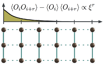
Figure 2: A universal resource deriving from the AKLT-model.

Several horizontal 1-D AKLT-type states can be coupled to become a universal 2-D resource. The coupling can be facilitated by performing a controlled-Z operation, embedded into the three-dimensional spin-1 space, between vertically adjacent nearest neighbors. More specifically, we will use the operation $\exp\{i\pi\mbox{$|2\rangle$}\mbox{$\langle 2|$}\otimes\mbox{$|2\rangle$}\mbox{$\langle 2|$}\}$, which introduces a $\pi$-phase between two systems exactly if both are in the state $|2\rangle$. The tensor network representation of this resource is given by

(126)

(133)

(140)

as one can check in analogy to Sec. III.5. Here,

$$H_{l\to r}:=\mbox{$|+\rangle$}_{r}\mbox{$\langle 0|$}_{l}+\mbox{$|-\rangle$}_{r}\mbox{$\langle 1|$}_{l}.$$ (141)

To verify that the resulting 2-D state constitutes a universal resource, we need to check that a) one can isolate the correlation system of a horizontal line from the rest of the lattice, so that it may be interpreted as a logical qubit and b) one can couple these logical qubits to perform an entangling gate.

The first step works in complete analogy to Section III.5, see Fig. 2. Indeed, one simply confirms that

$$\lx@xy@svg{\hbox{\raise 0.0pt\hbox{\kern 29.43732pt\hbox{{\hbox{\kern-29.43732pt\raise 0.0pt\hbox{\hbox{\kern 0.0pt\raise 24.53581pt\lx@xy@svgnested{\hbox{\raise 0.0pt\hbox{\kern 3.0pt\hbox{\ignorespaces\ignorespaces\ignorespaces\hbox{\vtop{\kern 0.0pt\offinterlineskip\halign{\entry@#!@&&\entry@@#!@\cr&&\\&&\\&&\\}}}\ignorespaces{\hbox{\kern-3.0pt\raise 0.0pt\hbox{\hbox{\kern 0.0pt\raise 0.0pt\hbox{\hbox{\kern 3.0pt\raise 0.0pt\hbox{$\textstyle{}$}}}}}}}{{{\hbox{\framed@@{0.0pt}}}}\hbox{\kern 11.53581pt\raise 0.0pt\hbox{\hbox{\kern 3.0pt\raise-2.5pt\hbox{$\textstyle{A[Z_{u}]}$}}}}}\ignorespaces\ignorespaces\ignorespaces\ignorespaces{}{\hbox{\lx@xy@droprule}}\ignorespaces{}{\hbox{\lx@xy@droprule}}{\hbox{\lx@xy@droprule}}{\hbox{\kern 49.87463pt\raise 0.0pt\hbox{\hbox{\kern 0.0pt\raise 0.0pt\hbox{\hbox{\kern 3.0pt\raise 0.0pt\hbox{$\textstyle{}$}}}}}}}{\hbox{\kern-3.0pt\raise-24.53581pt\hbox{\hbox{\kern 0.0pt\raise 0.0pt\hbox{\hbox{\kern 3.0pt\raise 0.0pt\hbox{$\textstyle{\ignorespaces\ignorespaces\ignorespaces\ignorespaces}$}}}}}}}\ignorespaces\ignorespaces\ignorespaces\ignorespaces{}{\hbox{\lx@xy@droprule}}\ignorespaces{\hbox{\kern 14.56578pt\raise-24.53581pt\hbox{\hbox{\kern 0.0pt\raise 0.0pt\hbox{\lx@xy@tip{1}\lx@xy@tip{-1}}}}}}{\hbox{\lx@xy@droprule}}{\hbox{\lx@xy@droprule}}{{{\hbox{\framed@@{0.0pt}}}}\hbox{\kern 14.56578pt\raise-24.53581pt\hbox{\hbox{\kern 3.0pt\raise-2.5pt\hbox{$\textstyle{A[s]}$}}}}}\ignorespaces\ignorespaces\ignorespaces\ignorespaces{}{\hbox{\lx@xy@droprule}}\ignorespaces{\hbox{\kern 49.87463pt\raise-24.53581pt\hbox{\hbox{\kern 0.0pt\raise 0.0pt\hbox{\lx@xy@tip{1}\lx@xy@tip{-1}}}}}}{\hbox{\lx@xy@droprule}}{\hbox{\lx@xy@droprule}}{\hbox{\kern 49.87463pt\raise-24.53581pt\hbox{\hbox{\kern 0.0pt\raise 0.0pt\hbox{\hbox{\kern 3.0pt\raise 0.0pt\hbox{$\textstyle{}$}}}}}}}{\hbox{\kern-3.0pt\raise-49.07162pt\hbox{\hbox{\kern 0.0pt\raise 0.0pt\hbox{\hbox{\kern 3.0pt\raise 0.0pt\hbox{$\textstyle{}$}}}}}}}{{{\hbox{\framed@@{0.0pt}}}}\hbox{\kern 12.24814pt\raise-49.07162pt\hbox{\hbox{\kern 3.0pt\raise-2.5pt\hbox{$\textstyle{A[Z_{l}]}$}}}}}\ignorespaces\ignorespaces\ignorespaces\ignorespaces{}{\hbox{\lx@xy@droprule}}\ignorespaces{}{\hbox{\lx@xy@droprule}}{\hbox{\lx@xy@droprule}}{\hbox{\kern 49.87463pt\raise-49.07162pt\hbox{\hbox{\kern 0.0pt\raise 0.0pt\hbox{\hbox{\kern 3.0pt\raise 0.0pt\hbox{$\textstyle{}$}}}}}}}\ignorespaces\ignorespaces}}}}}}}}}}}}=\pm\lx@xy@svg{\hbox{\raise 0.0pt\hbox{\kern 3.0pt\hbox{\ignorespaces\ignorespaces\ignorespaces\hbox{\vtop{\kern 0.0pt\offinterlineskip\halign{\entry@#!@&&\entry@@#!@\cr&&\crcr}}}\ignorespaces{\hbox{\kern-3.0pt\raise 0.0pt\hbox{\hbox{\kern 0.0pt\raise 0.0pt\hbox{\hbox{\kern 3.0pt\raise 0.0pt\hbox{$\textstyle{\ignorespaces\ignorespaces\ignorespaces\ignorespaces}$}}}}}}}\ignorespaces\ignorespaces\ignorespaces\ignorespaces{}{\hbox{\lx@xy@droprule}}\ignorespaces{\hbox{\kern 17.22636pt\raise 0.0pt\hbox{\hbox{\kern 0.0pt\raise 0.0pt\hbox{\lx@xy@tip{1}\lx@xy@tip{-1}}}}}}{\hbox{\lx@xy@droprule}}{\hbox{\lx@xy@droprule}}{{{\hbox{\framed@@{0.0pt}}}}\hbox{\kern 17.22636pt\raise 0.0pt\hbox{\hbox{\kern 3.0pt\raise-2.5pt\hbox{$\textstyle{A[s]}$}}}}}\ignorespaces\ignorespaces\ignorespaces\ignorespaces{}{\hbox{\lx@xy@droprule}}\ignorespaces{\hbox{\kern 55.1958pt\raise 0.0pt\hbox{\hbox{\kern 0.0pt\raise 0.0pt\hbox{\lx@xy@tip{1}\lx@xy@tip{-1}}}}}}{\hbox{\lx@xy@droprule}}{\hbox{\lx@xy@droprule}}{\hbox{\kern 55.1958pt\raise 0.0pt\hbox{\hbox{\kern 0.0pt\raise 0.0pt\hbox{\hbox{\kern 3.0pt\raise 0.0pt\hbox{$\textstyle{}$}}}}}}}\ignorespaces}}}}\ignorespaces, \textstyle{A[Z_{u}]} \textstyle{A[s]} \textstyle{A[Z_{l}]} \textstyle{A[s]} \textstyle{A[Z_{u}]} \textstyle{A[s]} \textstyle{A[Z_{l}]} \textstyle{A[s]}$$ (142)

where $s\in\{0,1,2\}$ and $Z_{u/l}$ denotes a measurement in the $\{\mbox{$|0\rangle$},\mbox{$|1\rangle$},\mbox{$|2\rangle$}\}$-basis. So measuring the vertically adjacent nodes in the computational basis gives us back the 1-D state, up to a possible sign.

A controlled-$Z$ gate can be realized in five steps:

$$\lx@xy@svg{\hbox{\raise 0.0pt\hbox{\kern 118.9916pt\hbox{{\hbox{\kern-118.9916pt\raise 0.0pt\hbox{\hbox{\kern 0.0pt\raise 35.1926pt\lx@xy@svgnested{\hbox{\raise 0.0pt\hbox{\kern 3.0pt\hbox{\ignorespaces\ignorespaces\ignorespaces\hbox{\vtop{\kern 0.0pt\offinterlineskip\halign{\entry@#!@&&\entry@@#!@\cr&&&&&\\&&&&&&\\&&&&&&\\&&&&&&\crcr}}}\ignorespaces{\hbox{\kern-3.0pt\raise 0.0pt\hbox{\hbox{\kern 0.0pt\raise 0.0pt\hbox{\hbox{\kern 3.0pt\raise 0.0pt\hbox{$\textstyle{}$}}}}}}}{\hbox{\kern 23.01111pt\raise 0.0pt\hbox{\hbox{\kern 0.0pt\raise 0.0pt\hbox{\hbox{\kern 3.0pt\raise 0.0pt\hbox{$\textstyle{-2}$}}}}}}}{\hbox{\kern 65.36247pt\raise 0.0pt\hbox{\hbox{\kern 0.0pt\raise 0.0pt\hbox{\hbox{\kern 3.0pt\raise 0.0pt\hbox{$\textstyle{-1}$}}}}}}}{\hbox{\kern 110.4916pt\raise 0.0pt\hbox{\hbox{\kern 0.0pt\raise 0.0pt\hbox{\hbox{\kern 3.0pt\raise 0.0pt\hbox{$\textstyle{0}$}}}}}}}{\hbox{\kern 152.84296pt\raise 0.0pt\hbox{\hbox{\kern 0.0pt\raise 0.0pt\hbox{\hbox{\kern 3.0pt\raise 0.0pt\hbox{$\textstyle{1}$}}}}}}}{\hbox{\kern 195.19432pt\raise 0.0pt\hbox{\hbox{\kern 0.0pt\raise 0.0pt\hbox{\hbox{\kern 3.0pt\raise 0.0pt\hbox{$\textstyle{2}$}}}}}}}{\hbox{\kern-3.0pt\raise-22.75803pt\hbox{\hbox{\kern 0.0pt\raise 0.0pt\hbox{\hbox{\kern 3.0pt\raise 0.0pt\hbox{$\textstyle{\ignorespaces\ignorespaces\ignorespaces\ignorespaces}$}}}}}}}\ignorespaces\ignorespaces\ignorespaces\ignorespaces{}{\hbox{\lx@xy@droprule}}\ignorespaces{\hbox{\kern 17.22636pt\raise-22.75803pt\hbox{\hbox{\kern 0.0pt\raise 0.0pt\hbox{\lx@xy@tip{1}\lx@xy@tip{-1}}}}}}{\hbox{\lx@xy@droprule}}{\hbox{\lx@xy@droprule}}{{{\hbox{\framed@@{0.0pt}}}}\hbox{\kern 17.22636pt\raise-22.75803pt\hbox{\hbox{\kern 3.0pt\raise-2.5pt\hbox{$\textstyle{A[X]}$}}}}}\ignorespaces\ignorespaces\ignorespaces\ignorespaces{}{\hbox{\lx@xy@droprule}}\ignorespaces{}{\hbox{\lx@xy@droprule}}{\hbox{\lx@xy@droprule}}{{{\hbox{\framed@@{0.0pt}}}}\hbox{\kern 59.57773pt\raise-22.75803pt\hbox{\hbox{\kern 3.0pt\raise-2.5pt\hbox{$\textstyle{A[X]}$}}}}}\ignorespaces\ignorespaces\ignorespaces\ignorespaces{}{\hbox{\lx@xy@droprule}}\ignorespaces{}{\hbox{\lx@xy@droprule}}{\hbox{\lx@xy@droprule}}{{{\hbox{\framed@@{0.0pt}}}}\hbox{\kern 101.9291pt\raise-22.75803pt\hbox{\hbox{\kern 3.0pt\raise-2.5pt\hbox{$\textstyle{A[X]}$}}}}}\ignorespaces\ignorespaces\ignorespaces\ignorespaces{}{\hbox{\lx@xy@droprule}}\ignorespaces{}{\hbox{\lx@xy@droprule}}{\hbox{\lx@xy@droprule}}{{{\hbox{\framed@@{0.0pt}}}}\hbox{\kern 144.28046pt\raise-22.75803pt\hbox{\hbox{\kern 3.0pt\raise-2.5pt\hbox{$\textstyle{A[X]}$}}}}}\ignorespaces\ignorespaces\ignorespaces\ignorespaces{}{\hbox{\lx@xy@droprule}}\ignorespaces{}{\hbox{\lx@xy@droprule}}{\hbox{\lx@xy@droprule}}{{{\hbox{\framed@@{0.0pt}}}}\hbox{\kern 186.63182pt\raise-22.75803pt\hbox{\hbox{\kern 3.0pt\raise-2.5pt\hbox{$\textstyle{A[X]}$}}}}}\ignorespaces\ignorespaces\ignorespaces\ignorespaces{}{\hbox{\lx@xy@droprule}}\ignorespaces{\hbox{\kern 228.98318pt\raise-22.75803pt\hbox{\hbox{\kern 0.0pt\raise 0.0pt\hbox{\lx@xy@tip{1}\lx@xy@tip{-1}}}}}}{\hbox{\lx@xy@droprule}}{\hbox{\lx@xy@droprule}}{\hbox{\kern 228.98318pt\raise-22.75803pt\hbox{\hbox{\kern 0.0pt\raise 0.0pt\hbox{\hbox{\kern 3.0pt\raise 0.0pt\hbox{$\textstyle{}$}}}}}}}{\hbox{\kern-3.0pt\raise-47.29384pt\hbox{\hbox{\kern 0.0pt\raise 0.0pt\hbox{\hbox{\kern 3.0pt\raise 0.0pt\hbox{$\textstyle{\ignorespaces\ignorespaces\ignorespaces\ignorespaces}$}}}}}}}\ignorespaces\ignorespaces\ignorespaces\ignorespaces{}{\hbox{\lx@xy@droprule}}\ignorespaces{\hbox{\kern 17.99023pt\raise-47.29384pt\hbox{\hbox{\kern 0.0pt\raise 0.0pt\hbox{\lx@xy@tip{1}\lx@xy@tip{-1}}}}}}{\hbox{\lx@xy@droprule}}{\hbox{\lx@xy@droprule}}{{{\hbox{\framed@@{0.0pt}}}}\hbox{\kern 17.99023pt\raise-47.29384pt\hbox{\hbox{\kern 3.0pt\raise-2.5pt\hbox{$\textstyle{A[Z]}$}}}}}\ignorespaces\ignorespaces\ignorespaces\ignorespaces{}{\hbox{\lx@xy@droprule}}\ignorespaces{}{\hbox{\lx@xy@droprule}}{\hbox{\lx@xy@droprule}}\ignorespaces\ignorespaces\ignorespaces\ignorespaces{}{\hbox{\lx@xy@droprule}}\ignorespaces{}{\hbox{\lx@xy@droprule}}{\hbox{\lx@xy@droprule}}\ignorespaces\ignorespaces\ignorespaces\ignorespaces{}{\hbox{\lx@xy@droprule}}\ignorespaces{}{\hbox{\lx@xy@droprule}}{\hbox{\lx@xy@droprule}}{{{\hbox{\framed@@{0.0pt}}}}\hbox{\kern 60.3416pt\raise-47.29384pt\hbox{\hbox{\kern 3.0pt\raise-2.5pt\hbox{$\textstyle{A[Z]}$}}}}}\ignorespaces\ignorespaces\ignorespaces\ignorespaces{}{\hbox{\lx@xy@droprule}}\ignorespaces{}{\hbox{\lx@xy@droprule}}{\hbox{\lx@xy@droprule}}\ignorespaces\ignorespaces\ignorespaces\ignorespaces{}{\hbox{\lx@xy@droprule}}\ignorespaces{}{\hbox{\lx@xy@droprule}}{\hbox{\lx@xy@droprule}}\ignorespaces\ignorespaces\ignorespaces\ignorespaces{}{\hbox{\lx@xy@droprule}}\ignorespaces{}{\hbox{\lx@xy@droprule}}{\hbox{\lx@xy@droprule}}{{{\hbox{\framed@@{0.0pt}}}}\hbox{\kern 102.4499pt\raise-47.29384pt\hbox{\hbox{\kern 3.0pt\raise-2.5pt\hbox{$\textstyle{A[Y]}$}}}}}\ignorespaces\ignorespaces\ignorespaces\ignorespaces{}{\hbox{\lx@xy@droprule}}\ignorespaces{}{\hbox{\lx@xy@droprule}}{\hbox{\lx@xy@droprule}}\ignorespaces\ignorespaces\ignorespaces\ignorespaces{}{\hbox{\lx@xy@droprule}}\ignorespaces{}{\hbox{\lx@xy@droprule}}{\hbox{\lx@xy@droprule}}\ignorespaces\ignorespaces\ignorespaces\ignorespaces{}{\hbox{\lx@xy@droprule}}\ignorespaces{}{\hbox{\lx@xy@droprule}}{\hbox{\lx@xy@droprule}}{{{\hbox{\framed@@{0.0pt}}}}\hbox{\kern 145.04433pt\raise-47.29384pt\hbox{\hbox{\kern 3.0pt\raise-2.5pt\hbox{$\textstyle{A[Z]}$}}}}}\ignorespaces\ignorespaces\ignorespaces\ignorespaces{}{\hbox{\lx@xy@droprule}}\ignorespaces{}{\hbox{\lx@xy@droprule}}{\hbox{\lx@xy@droprule}}\ignorespaces\ignorespaces\ignorespaces\ignorespaces{}{\hbox{\lx@xy@droprule}}\ignorespaces{}{\hbox{\lx@xy@droprule}}{\hbox{\lx@xy@droprule}}\ignorespaces\ignorespaces\ignorespaces\ignorespaces{}{\hbox{\lx@xy@droprule}}\ignorespaces{}{\hbox{\lx@xy@droprule}}{\hbox{\lx@xy@droprule}}{{{\hbox{\framed@@{0.0pt}}}}\hbox{\kern 187.39569pt\raise-47.29384pt\hbox{\hbox{\kern 3.0pt\raise-2.5pt\hbox{$\textstyle{A[Z]}$}}}}}\ignorespaces\ignorespaces\ignorespaces\ignorespaces{}{\hbox{\lx@xy@droprule}}\ignorespaces{}{\hbox{\lx@xy@droprule}}{\hbox{\lx@xy@droprule}}\ignorespaces\ignorespaces\ignorespaces\ignorespaces{}{\hbox{\lx@xy@droprule}}\ignorespaces{}{\hbox{\lx@xy@droprule}}{\hbox{\lx@xy@droprule}}\ignorespaces\ignorespaces\ignorespaces\ignorespaces{}{\hbox{\lx@xy@droprule}}\ignorespaces{\hbox{\kern 228.98318pt\raise-47.29384pt\hbox{\hbox{\kern 0.0pt\raise 0.0pt\hbox{\lx@xy@tip{1}\lx@xy@tip{-1}}}}}}{\hbox{\lx@xy@droprule}}{\hbox{\lx@xy@droprule}}{\hbox{\kern 228.98318pt\raise-47.29384pt\hbox{\hbox{\kern 0.0pt\raise 0.0pt\hbox{\hbox{\kern 3.0pt\raise 0.0pt\hbox{$\textstyle{}$}}}}}}}{\hbox{\kern-3.0pt\raise-71.82965pt\hbox{\hbox{\kern 0.0pt\raise 0.0pt\hbox{\hbox{\kern 3.0pt\raise 0.0pt\hbox{$\textstyle{\ignorespaces\ignorespaces\ignorespaces\ignorespaces}$}}}}}}}\ignorespaces\ignorespaces\ignorespaces\ignorespaces{}{\hbox{\lx@xy@droprule}}\ignorespaces{\hbox{\kern 17.22636pt\raise-71.82965pt\hbox{\hbox{\kern 0.0pt\raise 0.0pt\hbox{\lx@xy@tip{1}\lx@xy@tip{-1}}}}}}{\hbox{\lx@xy@droprule}}{\hbox{\lx@xy@droprule}}{{{\hbox{\framed@@{0.0pt}}}}\hbox{\kern 17.22636pt\raise-71.82965pt\hbox{\hbox{\kern 3.0pt\raise-2.5pt\hbox{$\textstyle{A[X]}$}}}}}\ignorespaces\ignorespaces\ignorespaces\ignorespaces{}{\hbox{\lx@xy@droprule}}\ignorespaces{}{\hbox{\lx@xy@droprule}}{\hbox{\lx@xy@droprule}}{{{\hbox{\framed@@{0.0pt}}}}\hbox{\kern 59.57773pt\raise-71.82965pt\hbox{\hbox{\kern 3.0pt\raise-2.5pt\hbox{$\textstyle{A[X]}$}}}}}\ignorespaces\ignorespaces\ignorespaces\ignorespaces{}{\hbox{\lx@xy@droprule}}\ignorespaces{}{\hbox{\lx@xy@droprule}}{\hbox{\lx@xy@droprule}}{{{\hbox{\framed@@{0.0pt}}}}\hbox{\kern 101.9291pt\raise-71.82965pt\hbox{\hbox{\kern 3.0pt\raise-2.5pt\hbox{$\textstyle{A[X]}$}}}}}\ignorespaces\ignorespaces\ignorespaces\ignorespaces{}{\hbox{\lx@xy@droprule}}\ignorespaces{}{\hbox{\lx@xy@droprule}}{\hbox{\lx@xy@droprule}}{{{\hbox{\framed@@{0.0pt}}}}\hbox{\kern 144.28046pt\raise-71.82965pt\hbox{\hbox{\kern 3.0pt\raise-2.5pt\hbox{$\textstyle{A[X]}$}}}}}\ignorespaces\ignorespaces\ignorespaces\ignorespaces{}{\hbox{\lx@xy@droprule}}\ignorespaces{}{\hbox{\lx@xy@droprule}}{\hbox{\lx@xy@droprule}}{{{\hbox{\framed@@{0.0pt}}}}\hbox{\kern 186.63182pt\raise-71.82965pt\hbox{\hbox{\kern 3.0pt\raise-2.5pt\hbox{$\textstyle{A[X]}$}}}}}\ignorespaces\ignorespaces\ignorespaces\ignorespaces{}{\hbox{\lx@xy@droprule}}\ignorespaces{\hbox{\kern 228.98318pt\raise-71.82965pt\hbox{\hbox{\kern 0.0pt\raise 0.0pt\hbox{\lx@xy@tip{1}\lx@xy@tip{-1}}}}}}{\hbox{\lx@xy@droprule}}{\hbox{\lx@xy@droprule}}{\hbox{\kern 228.98318pt\raise-71.82965pt\hbox{\hbox{\kern 0.0pt\raise 0.0pt\hbox{\hbox{\kern 3.0pt\raise 0.0pt\hbox{$\textstyle{}$}}}}}}}\ignorespaces\ignorespaces}}}}}}}}}}}}. \textstyle{-2} \textstyle{-1} \textstyle{0} \textstyle{1} \textstyle{2} \textstyle{A[X]} \textstyle{A[X]} \textstyle{A[X]} \textstyle{A[X]} \textstyle{A[X]} \textstyle{A[Z]} \textstyle{A[Z]} \textstyle{A[Y]} \textstyle{A[Z]} \textstyle{A[Z]} \textstyle{A[X]} \textstyle{A[X]} \textstyle{A[X]} \textstyle{A[X]} \textstyle{A[X]} \textstyle{-2} \textstyle{-1} \textstyle{0} \textstyle{1} \textstyle{2} \textstyle{A[X]} \textstyle{A[X]} \textstyle{A[X]} \textstyle{A[X]} \textstyle{A[X]} \textstyle{A[Z]} \textstyle{A[Z]} \textstyle{A[Y]} \textstyle{A[Z]} \textstyle{A[Z]} \textstyle{A[X]} \textstyle{A[X]} \textstyle{A[X]} \textstyle{A[X]} \textstyle{A[X]}$$ (151)

The Pauli matrices $X,Y,Z$ are understood as being embedded into the $\{\mbox{$|1\rangle$},\mbox{$|2\rangle$}\}$-subspace. So, e.g., $X$ denotes a measurement in the $\{\mbox{$|0\rangle$},2^{-1/2}(\mbox{$|1\rangle$}\pm\mbox{$|2\rangle$})\}$-basis. When operating the gate, we first measure all sites of the upper and lower lines in the $X$-eigenbasis. In case the result for the sites at position “0” (refer to labeling above) is different from $|+\rangle$, the gate failed. In that case all sites on the middle line are measured in the computational basis and we restart the procedure five steps to the right. Otherwise, the systems labeled by a $Z$ are measured. We accept the outcome only if we obtained $|1\rangle$ on sites $\pm 2$ and $|0\rangle$ on sites $\pm 1$ – should a different result occur, the gate is once again considered a failure and we proceed as above. Lastly, the $Y$ measurement on the central site is performed. In case of a result corresponding to $|0\rangle$, it is easy to see that no interaction between the upper and the lower part takes place, so this is the last possibility for the gate to fail. Let us assume now that the desired measurement outcomes were realized. At site $-2$ on the middle line, we obtained

$$\lx@xy@svg{\hbox{\raise 0.0pt\hbox{\kern 12.0278pt\hbox{\ignorespaces\ignorespaces\ignorespaces\hbox{\vtop{\kern 0.0pt\offinterlineskip\halign{\entry@#!@&&\entry@@#!@\cr&\crcr}}}\ignorespaces{{{\hbox{\framed@@{0.0pt}}}}\hbox{\kern-12.0278pt\raise 0.0pt\hbox{\hbox{\kern 3.0pt\raise-2.5pt\hbox{$\textstyle{A[1]}$}}}}}\ignorespaces\ignorespaces\ignorespaces\ignorespaces{}{\hbox{\lx@xy@droprule}}\ignorespaces{\hbox{\kern 26.25417pt\raise 0.0pt\hbox{\hbox{\kern 0.0pt\raise 0.0pt\hbox{\lx@xy@tip{1}\lx@xy@tip{-1}}}}}}{\hbox{\lx@xy@droprule}}{\hbox{\lx@xy@droprule}}{\hbox{\kern 26.25417pt\raise 0.0pt\hbox{\hbox{\kern 0.0pt\raise 0.0pt\hbox{\hbox{\kern 3.0pt\raise 0.0pt\hbox{$\textstyle{}$}}}}}}}\ignorespaces}}}}\ignorespaces, \textstyle{A[1]} \textstyle{A[1]}$$ (153)

which prepares the correlation system of the middle line in $|0\rangle$. At site $-1$, in turn, a Hadamard gate has been realized, which causes the output of site $-1$ to be $H\mbox{$|0\rangle$}=\mbox{$|+\rangle$}$. The situation is similar on the r.h.s., so that the above network at site $0$ can be re-written as

$$\lx@xy@svg{\hbox{\raise 0.0pt\hbox{\kern 41.54585pt\hbox{{\hbox{\kern-41.54585pt\raise 0.0pt\hbox{\hbox{\kern 0.0pt\raise 24.53581pt\lx@xy@svgnested{\hbox{\raise 0.0pt\hbox{\kern 6.8889pt\hbox{\ignorespaces\ignorespaces\ignorespaces\hbox{\vtop{\kern 0.0pt\offinterlineskip\halign{\entry@#!@&&\entry@@#!@\cr&&\\&&\\&&\\}}}\ignorespaces{\hbox{\kern-3.0pt\raise 0.0pt\hbox{\hbox{\kern 0.0pt\raise 0.0pt\hbox{\hbox{\kern 3.0pt\raise 0.0pt\hbox{$\textstyle{\ignorespaces\ignorespaces\ignorespaces\ignorespaces}$}}}}}}}\ignorespaces\ignorespaces\ignorespaces\ignorespaces{}{\hbox{\lx@xy@droprule}}\ignorespaces{\hbox{\kern 21.24026pt\raise 0.0pt\hbox{\hbox{\kern 0.0pt\raise 0.0pt\hbox{\lx@xy@tip{1}\lx@xy@tip{-1}}}}}}{\hbox{\lx@xy@droprule}}{\hbox{\lx@xy@droprule}}{{{\hbox{\framed@@{0.0pt}}}}\hbox{\kern 21.24026pt\raise 0.0pt\hbox{\hbox{\kern 3.0pt\raise-2.5pt\hbox{$\textstyle{A[+]}$}}}}}\ignorespaces\ignorespaces\ignorespaces\ignorespaces{}{\hbox{\lx@xy@droprule}}\ignorespaces{\hbox{\kern 66.3139pt\raise 0.0pt\hbox{\hbox{\kern 0.0pt\raise 0.0pt\hbox{\lx@xy@tip{1}\lx@xy@tip{-1}}}}}}{\hbox{\lx@xy@droprule}}{\hbox{\lx@xy@droprule}}{\hbox{\kern 66.3139pt\raise 0.0pt\hbox{\hbox{\kern 0.0pt\raise 0.0pt\hbox{\hbox{\kern 3.0pt\raise 0.0pt\hbox{$\textstyle{}$}}}}}}}{{{\hbox{\framed@@{0.0pt}}}}\hbox{\kern-6.8889pt\raise-24.53581pt\hbox{\hbox{\kern 3.0pt\raise-2.5pt\hbox{$\textstyle{+}$}}}}}\ignorespaces\ignorespaces\ignorespaces\ignorespaces{}{\hbox{\lx@xy@droprule}}\ignorespaces{}{\hbox{\lx@xy@droprule}}{\hbox{\lx@xy@droprule}}{{{\hbox{\framed@@{0.0pt}}}}\hbox{\kern 21.11526pt\raise-24.53581pt\hbox{\hbox{\kern 3.0pt\raise-2.5pt\hbox{$\textstyle{A[Y]}$}}}}}\ignorespaces\ignorespaces\ignorespaces\ignorespaces{}{\hbox{\lx@xy@droprule}}\ignorespaces{}{\hbox{\lx@xy@droprule}}{\hbox{\lx@xy@droprule}}\ignorespaces\ignorespaces\ignorespaces\ignorespaces{}{\hbox{\lx@xy@droprule}}\ignorespaces{}{\hbox{\lx@xy@droprule}}{\hbox{\lx@xy@droprule}}{{{\hbox{\framed@@{0.0pt}}}}\hbox{\kern 62.425pt\raise-24.53581pt\hbox{\hbox{\kern 3.0pt\raise-2.5pt\hbox{$\textstyle{+}$}}}}}{\hbox{\kern-3.0pt\raise-49.07162pt\hbox{\hbox{\kern 0.0pt\raise 0.0pt\hbox{\hbox{\kern 3.0pt\raise 0.0pt\hbox{$\textstyle{\ignorespaces\ignorespaces\ignorespaces\ignorespaces}$}}}}}}}\ignorespaces\ignorespaces\ignorespaces\ignorespaces{}{\hbox{\lx@xy@droprule}}\ignorespaces{\hbox{\kern 21.24026pt\raise-49.07162pt\hbox{\hbox{\kern 0.0pt\raise 0.0pt\hbox{\lx@xy@tip{1}\lx@xy@tip{-1}}}}}}{\hbox{\lx@xy@droprule}}{\hbox{\lx@xy@droprule}}{{{\hbox{\framed@@{0.0pt}}}}\hbox{\kern 21.24026pt\raise-49.07162pt\hbox{\hbox{\kern 3.0pt\raise-2.5pt\hbox{$\textstyle{A[+]}$}}}}}\ignorespaces\ignorespaces\ignorespaces\ignorespaces{}{\hbox{\lx@xy@droprule}}\ignorespaces{\hbox{\kern 66.3139pt\raise-49.07162pt\hbox{\hbox{\kern 0.0pt\raise 0.0pt\hbox{\lx@xy@tip{1}\lx@xy@tip{-1}}}}}}{\hbox{\lx@xy@droprule}}{\hbox{\lx@xy@droprule}}\ignorespaces\ignorespaces\ignorespaces\ignorespaces{}{\hbox{\lx@xy@droprule}}\ignorespaces{}{\hbox{\lx@xy@droprule}}{\hbox{\lx@xy@droprule}}{\hbox{\kern 66.3139pt\raise-49.07162pt\hbox{\hbox{\kern 0.0pt\raise 0.0pt\hbox{\hbox{\kern 3.0pt\raise 0.0pt\hbox{$\textstyle{}$}}}}}}}\ignorespaces\ignorespaces}}}}}}}}}}}}. \textstyle{A[+]} \textstyle{+} \textstyle{A[Y]} \textstyle{+} \textstyle{A[+]} \textstyle{A[+]} \textstyle{+} \textstyle{A[Y]} \textstyle{+} \textstyle{A[+]}$$ (154)

We will now analyze the tensor network in Eq. (154) step by step. For proving its functionality, there is no loss of generality in restricting attention to the situation where the correlation system of the lower line is initially in state $|c\rangle$, for $c\in\{0,1\}$. We compute for the lower part of the tensor network

$$\lx@xy@svg{\hbox{\raise 0.0pt\hbox{\kern 40.25125pt\hbox{{\hbox{\kern-40.25125pt\raise 0.0pt\hbox{\hbox{\kern 0.0pt\raise 12.26791pt\lx@xy@svgnested{\hbox{\raise 0.0pt\hbox{\kern 9.6082pt\hbox{\ignorespaces\ignorespaces\ignorespaces\hbox{\vtop{\kern 0.0pt\offinterlineskip\halign{\entry@#!@&&\entry@@#!@\cr&&\\&&\crcr}}}\ignorespaces{\hbox{\kern-3.0pt\raise 0.0pt\hbox{\hbox{\kern 0.0pt\raise 0.0pt\hbox{\hbox{\kern 3.0pt\raise 0.0pt\hbox{$\textstyle{}$}}}}}}}{\hbox{\kern 34.25125pt\raise 0.0pt\hbox{\hbox{\kern 0.0pt\raise 0.0pt\hbox{\hbox{\kern 3.0pt\raise 0.0pt\hbox{$\textstyle{}$}}}}}}}{\hbox{\kern 64.8943pt\raise 0.0pt\hbox{\hbox{\kern 0.0pt\raise 0.0pt\hbox{\hbox{\kern 3.0pt\raise 0.0pt\hbox{$\textstyle{}$}}}}}}}{{{\hbox{\framed@@{0.0pt}}}}\hbox{\kern-9.6082pt\raise-19.53581pt\hbox{\hbox{\kern 3.0pt\raise-2.5pt\hbox{$\textstyle{\mbox{$|c\rangle$}}$}}}}}\ignorespaces\ignorespaces\ignorespaces\ignorespaces{}{\hbox{\lx@xy@droprule}}\ignorespaces{}{\hbox{\lx@xy@droprule}}{\hbox{\lx@xy@droprule}}{{{\hbox{\framed@@{0.0pt}}}}\hbox{\kern 23.83456pt\raise-19.53581pt\hbox{\hbox{\kern 3.0pt\raise-2.5pt\hbox{$\textstyle{A[+]}$}}}}}\ignorespaces\ignorespaces\ignorespaces\ignorespaces{}{\hbox{\lx@xy@droprule}}\ignorespaces{\hbox{\kern 64.8943pt\raise-19.53581pt\hbox{\hbox{\kern 0.0pt\raise 0.0pt\hbox{\lx@xy@tip{1}\lx@xy@tip{-1}}}}}}{\hbox{\lx@xy@droprule}}{\hbox{\lx@xy@droprule}}\ignorespaces\ignorespaces\ignorespaces\ignorespaces{}{\hbox{\lx@xy@droprule}}\ignorespaces{\hbox{\kern 37.25125pt\raise-3.0pt\hbox{\hbox{\kern 0.0pt\raise 0.0pt\hbox{\lx@xy@tip{1}\lx@xy@tip{-1}}}}}}{\hbox{\lx@xy@droprule}}{\hbox{\lx@xy@droprule}}{\hbox{\kern 64.8943pt\raise-19.53581pt\hbox{\hbox{\kern 0.0pt\raise 0.0pt\hbox{\hbox{\kern 3.0pt\raise 0.0pt\hbox{$\textstyle{}$}}}}}}}\ignorespaces\ignorespaces}}}}}}}}}}}}=X\mbox{$|c\rangle$}_{r}Z^{c}\mbox{$|+\rangle$}_{u}. |c\rangle \textstyle{A[+]} |c\rangle \textstyle{A[+]}$$ (155)

Further, plugging the output $Z^{c}\mbox{$|+\rangle$}$ of the lower stage into the middle part, we find

$$\lx@xy@svg{\hbox{\raise 0.0pt\hbox{\kern 43.20895pt\hbox{{\hbox{\kern-43.20895pt\raise 0.0pt\hbox{\hbox{\kern 0.0pt\raise 24.80524pt\lx@xy@svgnested{\hbox{\raise 0.0pt\hbox{\kern 6.8889pt\hbox{\ignorespaces\ignorespaces\ignorespaces\hbox{\vtop{\kern 0.0pt\offinterlineskip\halign{\entry@#!@&&\entry@@#!@\cr&&\\&&\\&\crcr}}}\ignorespaces{\hbox{\kern-3.0pt\raise 0.0pt\hbox{\hbox{\kern 0.0pt\raise 0.0pt\hbox{\hbox{\kern 3.0pt\raise 0.0pt\hbox{$\textstyle{}$}}}}}}}{\hbox{\kern 33.32005pt\raise 0.0pt\hbox{\hbox{\kern 0.0pt\raise 0.0pt\hbox{\hbox{\kern 3.0pt\raise 0.0pt\hbox{$\textstyle{}$}}}}}}}{\hbox{\kern 69.6401pt\raise 0.0pt\hbox{\hbox{\kern 0.0pt\raise 0.0pt\hbox{\hbox{\kern 3.0pt\raise 0.0pt\hbox{$\textstyle{}$}}}}}}}{{{\hbox{\framed@@{0.0pt}}}}\hbox{\kern-6.8889pt\raise-19.53581pt\hbox{\hbox{\kern 3.0pt\raise-2.5pt\hbox{$\textstyle{+}$}}}}}\ignorespaces\ignorespaces\ignorespaces\ignorespaces{}{\hbox{\lx@xy@droprule}}\ignorespaces{}{\hbox{\lx@xy@droprule}}{\hbox{\lx@xy@droprule}}{{{\hbox{\framed@@{0.0pt}}}}\hbox{\kern 22.77837pt\raise-19.53581pt\hbox{\hbox{\kern 3.0pt\raise-2.5pt\hbox{$\textstyle{A[Y]}$}}}}}\ignorespaces\ignorespaces\ignorespaces\ignorespaces{}{\hbox{\lx@xy@droprule}}\ignorespaces{}{\hbox{\lx@xy@droprule}}{\hbox{\lx@xy@droprule}}\ignorespaces\ignorespaces\ignorespaces\ignorespaces{}{\hbox{\lx@xy@droprule}}\ignorespaces{\hbox{\kern 36.32005pt\raise-3.0pt\hbox{\hbox{\kern 0.0pt\raise 0.0pt\hbox{\lx@xy@tip{1}\lx@xy@tip{-1}}}}}}{\hbox{\lx@xy@droprule}}{\hbox{\lx@xy@droprule}}{{{\hbox{\framed@@{0.0pt}}}}\hbox{\kern 65.7512pt\raise-19.53581pt\hbox{\hbox{\kern 3.0pt\raise-2.5pt\hbox{$\textstyle{+}$}}}}}{\hbox{\kern-3.0pt\raise-44.34105pt\hbox{\hbox{\kern 0.0pt\raise 0.0pt\hbox{\hbox{\kern 3.0pt\raise 0.0pt\hbox{$\textstyle{}$}}}}}}}{{{\hbox{\framed@@{0.0pt}}}}\hbox{\kern 21.11526pt\raise-44.34105pt\hbox{\hbox{\kern 3.0pt\raise-2.76944pt\hbox{$\textstyle{Z^{c}\mbox{$|+\rangle$}}$}}}}}\ignorespaces\ignorespaces\ignorespaces\ignorespaces{}{\hbox{\lx@xy@droprule}}\ignorespaces{}{\hbox{\lx@xy@droprule}}{\hbox{\lx@xy@droprule}}\ignorespaces\ignorespaces}}}}}}}}}}}}\propto Z^{c+y}(\mbox{$|0\rangle$}+i\mbox{$|1\rangle$}), \textstyle{+} \textstyle{A[Y]} \textstyle{+} \textstyle{Z^{c}\mbox{$|+\rangle$}} \textstyle{+} \textstyle{A[Y]} \textstyle{+} \textstyle{Z^{c}\mbox{$|+\rangle$}}$$ (156)

where $y\in 0,1$ reflects the outcome of the $Y$-measurement on the central site: $y=0$ in case of $\mbox{$|1\rangle$}+i\mbox{$|2\rangle$}$ and $y=1$ for $\mbox{$|1\rangle$}-i\mbox{$|2\rangle$}$. Lastly,

$$\lx@xy@svg{\hbox{\raise 0.0pt\hbox{\kern 56.36026pt\hbox{{\hbox{\kern-56.36026pt\raise 0.0pt\hbox{\hbox{\kern 0.0pt\raise 12.75122pt\lx@xy@svgnested{\hbox{\raise 0.0pt\hbox{\kern 3.0pt\hbox{\ignorespaces\ignorespaces\ignorespaces\hbox{\vtop{\kern 0.0pt\offinterlineskip\halign{\entry@#!@&&\entry@@#!@\cr&&\\&\crcr}}}\ignorespaces{\hbox{\kern-3.0pt\raise 0.0pt\hbox{\hbox{\kern 0.0pt\raise 0.0pt\hbox{\hbox{\kern 3.0pt\raise 0.0pt\hbox{$\textstyle{\ignorespaces\ignorespaces\ignorespaces\ignorespaces}$}}}}}}}\ignorespaces\ignorespaces\ignorespaces\ignorespaces{}{\hbox{\lx@xy@droprule}}\ignorespaces{\hbox{\kern 39.94357pt\raise 0.0pt\hbox{\hbox{\kern 0.0pt\raise 0.0pt\hbox{\lx@xy@tip{1}\lx@xy@tip{-1}}}}}}{\hbox{\lx@xy@droprule}}{\hbox{\lx@xy@droprule}}{{{\hbox{\framed@@{0.0pt}}}}\hbox{\kern 39.94357pt\raise 0.0pt\hbox{\hbox{\kern 3.0pt\raise-2.5pt\hbox{$\textstyle{A[+]}$}}}}}\ignorespaces\ignorespaces\ignorespaces\ignorespaces{}{\hbox{\lx@xy@droprule}}\ignorespaces{\hbox{\kern 103.72052pt\raise 0.0pt\hbox{\hbox{\kern 0.0pt\raise 0.0pt\hbox{\lx@xy@tip{1}\lx@xy@tip{-1}}}}}}{\hbox{\lx@xy@droprule}}{\hbox{\lx@xy@droprule}}{\hbox{\kern 103.72052pt\raise 0.0pt\hbox{\hbox{\kern 0.0pt\raise 0.0pt\hbox{\hbox{\kern 3.0pt\raise 0.0pt\hbox{$\textstyle{}$}}}}}}}{\hbox{\kern-3.0pt\raise-25.01913pt\hbox{\hbox{\kern 0.0pt\raise 0.0pt\hbox{\hbox{\kern 3.0pt\raise 0.0pt\hbox{$\textstyle{}$}}}}}}}{{{\hbox{\framed@@{0.0pt}}}}\hbox{\kern 17.22636pt\raise-25.01913pt\hbox{\hbox{\kern 3.0pt\raise-2.98332pt\hbox{$\textstyle{Z^{c+y}(\mbox{$|0\rangle$}+i\mbox{$|1\rangle$})}$}}}}}\ignorespaces\ignorespaces\ignorespaces\ignorespaces{}{\hbox{\lx@xy@droprule}}\ignorespaces{}{\hbox{\lx@xy@droprule}}{\hbox{\lx@xy@droprule}}\ignorespaces\ignorespaces}}}}}}}}}}}}\propto SZ^{c+y}X. \textstyle{A[+]} \textstyle{Z^{c+y}(\mbox{$|0\rangle$}+i\mbox{$|1\rangle$})} \textstyle{A[+]} \textstyle{Z^{c+y}(\mbox{$|0\rangle$}+i\mbox{$|1\rangle$})}$$ (157)

In summary, the evolution afforded on the upper line is $HSZ^{y+c}$, equivalent to $Z^{c}$ up to by-products. This completes the proof of universality.

For completeness, note that we never need the by-products to vanish for all logical qubits of the full computation simultaneously. Hence the expected number of steps for the realization of one- or two-qubit gates is a constant in the number of total logical qubits.

IV.2 Toric code states

In the following, we present two MBQC resource states which are motivated by Kitaev’s toric code states [38]. This contrasts with a result in Ref. [34] that MBQC on the planar toric code state itself can be simulated efficiently classically. Different from the other schemes presented, the natural gate in these schemes is a two-qubit interaction, whereas local operations have to be implemented indirectly. Also, individual qubits are decoupled not by erasing sites but by switching off the coupling between them.

Toric code states are states with non-trivial topological properties and have been introduced in the context of quantum error correction. They have a particularly simple representation in terms of PEPS [39] or CTNs [1] on two centered square lattices,

(158)

where

(173)

and

(186)

i.e., $K_{H}$ and $K_{V}$ are identical up to a rotation by $90$ degrees.

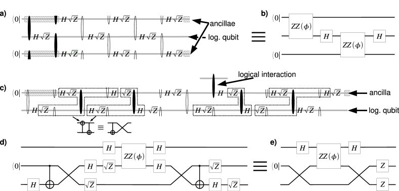
Figure 3: Implementation of single-qubit and two-qubit operations in the first toric code model. a) The measurement pattern for single-qubit operations and b) the corresponding circuit. c) Pattern for a two-qubit gate between logical qubits, d) the corresponding circuit and e) the circuit after some simplifications.

Let us first see how $K_{H}$ acts on two qubits in correlation space coming from the left. The most basic operation is a measurement in the computational basis, which simply transports both qubits to the right (up to a correlated $Z$ by-product operator). Generalizing this to measurements in the $Y$-$Z$ plane, we find that

(199)

where $\phi$ is the angle with the $Z$ axis, and

$$ZZ(\phi)=\left(\begin{array}[]{cccc}1\\ &e^{i\phi}\\ &&e^{i\phi}\\ &&&1\end{array}\right)\ .$$ (200)

(Note that this gate is locally equivalent to the cnot gate for $\phi=\pm\pi/2$.)

Thus, the tensors in Kitaev’s toric code state have a two-qubit operation as their natural gate in correlation space, rather than a single-qubit gate. In MBQC schemes which base on these projectors, two-qubit gates are easy to realize, whereas in order to get one-qubit gates, tricks have to be used. In the first example, we obtain single-qubit operations by introducing ancillae: a $ZZ$ controlled phase between a logical qubit and an ancilla in a computational basis state yields a local $Z$ rotation on the logical qubit. In the second example, we use a different approach: we encode each logical qubit in two qubits in correlation space. Using this nonlocal encoding, we obtain an easy implementation of both one- and two-qubit operations; furthermore, the scheme allows for an arbitrary parallelization of the two-qubit interactions.

Observation 6 (Logical qubits in several correlation systems).

There is no need to have a one-one correspondance between logical qubits and a single correlation system.

IV.2.1 Toric codes: first scheme

Our first scheme consists of the modified tensor

(215)

$$= \textstyle{\hskip 11.99998ptZ^{s}\hskip 11.99998pt} \textstyle{\sqrt{Z}HZ^{s}}$$ (224)

[with $\sqrt{Z}=\mathrm{diag}(1,i)$], arranged as in (158) where both $K_{H}$ and $K_{V}$ are replaced by $\tilde{K}_{H}$. The extra $H$ serves the same purpose as in other schemes: it allows to leave the subspace of diagonal operations and thus to implement $X$ rotations. The need for the $\sqrt{Z}$ will become clear later; it is connected to the fact that

$$\mbox{\sc cnot}=(\mathbbm{1}\otimes H)\;(\sqrt{Z}\otimes\sqrt{Z})\;ZZ(-\pi/2)\;(\mathbbm{1}\otimes H)\ .$$ (225)

In the following, we show how this state can be used for MBQC. The qubits run from left to right in correlation space in zig-zag lines in Eq. (158); for the illustration in Fig. 3, we have straightened these lines, and marked the measurement-induced $ZZ$ interactions coming from the $K_{H}[s]$ in (215) by ellipses. (The difference between filled and non-filled ellipses will be explained later.) The $\sqrt{Z}H$ operations of (215) do not depend on the measurement and are thus hard-wired; note that the order is reversed as we are considering $H$ and $\sqrt{Z}$ as two independent operations in the circuit.

Let us first impose that all qubits are initialized to $|0\rangle$; this corresponds to a left boundary condition $|0\rangle$ in correlation space. We will discuss later how to initialize the scheme. Every second qubit is an ancilla which will be used to implement one-qubit operations. We first discuss the case of no Pauli errors, and show later how those can be dealt with.

The implementation of single-qubit operations is illustrated in Fig. 3a. There, each ellipse denotes a possible $ZZ$ interaction. In particular, empty ellipses denote interactions which are switched off (i.e. measured in the $Z$ basis), while filled ellipses denote sites where one can measure in the $Y$-$Z$ plane to implement a $ZZ$ gate. If all interactions are switched off, all qubits are transported to the right, subject to the transformation $\sqrt{Z}H$. As $(\sqrt{Z}H)^{3}=\mathbbm{1}$, the ancillae are in the computational basis in every third step: These regions are hashed in Fig. 3a. In these regions, a $ZZ(\phi)$ between ancilla and logical qubit (corresponding to the filled ellipses in the figure) results in a single-qubit $Z$ rotation on the latter. Thus, in each block of length three as the one shown in Fig. 3a, the transformation

$$\sqrt{Z}H\sqrt{Z}HS(\psi)\sqrt{Z}HS(\phi)=HS(\psi)HS(\phi)$$ (226)

is implemented [where $S(\phi)=\mathrm{diag}(1,e^{i\phi})$], which allows for arbitrary one-qubit operations. In Fig. 3b, the corresponding circuit is shown, which has been simplified using $H\sqrt{Z}H\sqrt{Z}=\sqrt{X}\sqrt{Z}=(\sqrt{Z})^{-1}H$, and that diagonal matrices commute.

Although the scheme has a natural two-qubit interaction, implementing an interaction between two adjacent logical qubits is complicated by the ancilla which is located inbetween. In order to obtain a coupling, we first swap the logical qubit with the ancilla, then couple it to the now adjacent logical neighbor, and finally swap it back. This is implemented by the measurement pattern shown in Fig. 3c. Again, empty ellipses correspond to switched off interactions, while the filled ellipses all implement $ZZ(-\pi/2)$ gates, each of which together with two $\sqrt{Z}$ and two Hadamards as grouped in the figure gives a cnot gate, cf. Eq. (225). This measurement pattern corresponds to the circuit shown in Fig. 3d, where we have replaced each pair of cnots by a cnot and a swap. By merging each cnot with the two adjacent Hadamards, we effectively obtain

$$CZ=|0,0\rangle\langle 0,0|+|0,1\rangle\langle 0,1|+|1,0\rangle\langle 1,0|-|1,1\rangle\langle 1,1|$$ (227)

gates. We thus remain with only diagonal gates on the two lower qubits (except for the swap), i.e. the gates all commute and the circuit can thus be simplified to the one shown on in Fig. 3e, proving that the sequence effectively implements a two-qubit interaction between the logical qubits. Note that the length of the complete sequence is compatible with the three-periodicity of the basis of the ancillae.

Pauli errors in this scheme can be dealt with as usual: $H$ and $\sqrt{Z}$ are both in the Clifford group, i.e., Paulis can be commuted through, and $ZZ$ commutes with $Z$ errors, while $(\mathbbm{1}\otimes X)ZZ(\phi)=ZZ(-\phi)(\mathbbm{1}\otimes X)$.

Finally, we show how to read out the logical qubits. It holds that

(242)

(257)

i.e., a measurement in the $X$ basis returns the parity of the ancilla and the logical qubit. If this is done when the ancilla is in a computational basis state, one effectively measures the logical qubit in the computational basis. Note that both the ancilla and the logical qubit are in a well-defined state afterwards and can thus be reused.

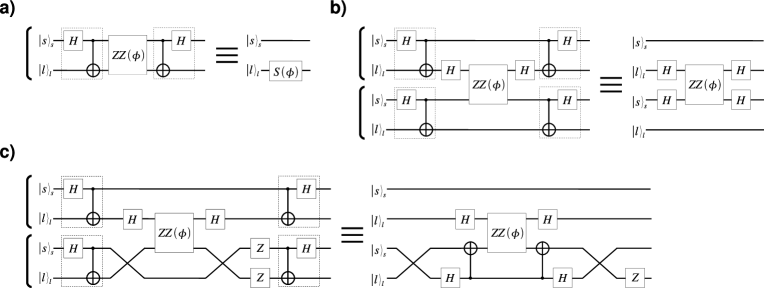
Figure 4: Interpretation of the first toric code scheme in terms of parity encoded qubits. The boxed parts of the circuit decode and encode the system. a) $Z$ rotations result in $Z$ rotations in the encoded system. b) $X$ rotations result in $X$ rotations in the encoded system, plus $Z$ corrections before and after the rotations in case the $s$ qubit below is $\mbox{$|-\rangle$}_{s}$ rather than $\mbox{$|+\rangle$}_{s}$. c) Similarly, the coupling circuit Fig. 3d results in a coupling of the encoded logical qubits, up to the same $Z$ correction on the first logical qubit which depends on the $s$ qubit below in exactly the same way. Thus, the $Z$ corrections on each qubit cancel out except for the first and the last, which have no effect due to the initialization and measurement in the computational basis.

Let us now turn towards the initialization procedure. In contrast to the previous MBQC schemes, the read-out cannot be used for initialization. The reason is that the read-out only works if the ancilla qubit is initially in a computational basis state; otherwise, it just projects onto the subspace spanned by $\{\mbox{$|0,0\rangle$},\mbox{$|1,1\rangle$}\}$ or by $\{\mbox{$|0,1\rangle$},\mbox{$|1,0\rangle$}\}$.

In the following, we demonstrate that it is still possible to initialize this scheme by taking a different perspective on how it encodes logical qubits. Therefore, we group each logical qubit with the ancilla above (e.g., the first two qubits in Fig. 3a), and encode the new logical qubit in their parity – note that this is what is really measured in the read-out. The following calculations are most conveniently carried out in a Bell basis where each state is described as $\mbox{$|s\rangle$}_{s}\mbox{$|l\rangle$}_{l}$, where the $s$ qubit stores the sign of the Bell state and the $l$ qubit the parity and thus encodes our logical qubit, i.e.

$$\mbox{$|s\rangle$}_{s}\mbox{$|0\rangle$}_{l} \leftrightarrow \mbox{$|0,0\rangle$}+(-1)^{s}\mbox{$|1,1\rangle$}$$ (258)

$$\mbox{$|s\rangle$}_{s}\mbox{$|1\rangle$}_{l} \leftrightarrow \mbox{$|0,1\rangle$}+(-1)^{s}\mbox{$|1,0\rangle$}\ .$$ (259)

The circuit transforming between the above encoding and the qubits in correlation space is

$$\includegraphics[height=34.14322pt]{toric3n}\ \ .$$ (260)

Using this decoding, it is straightforward to investigate what happens in the various steps of the MBQC scheme. Firstly, one can easily check that by measuring two consecutive couplings of the qubit pair in the $X$ basis, one prepares them in a maximally entangled state $\mbox{$|0,0\rangle$}+\mbox{$|1,1\rangle$}$ up to Pauli errors, corresponding to $\mbox{$|0\rangle$}_{s}\mbox{$|0\rangle$}_{l}$ in the encoded system. By pretending a Pauli $Z$ error on one of the qubits with $p=1/2$, we effectively face the mixture $\mbox{$|0,0\rangle$}\mbox{$\langle 0,0|$}+\mbox{$|1,1\rangle$}\mbox{$\langle 1,1|$}$, corresponding to $\mathbbm{1}_{s}\otimes\mbox{$|0\rangle$}\mbox{$\langle 0|$}_{l}$.

Since the transformation (260) is in the Clifford group, Pauli errors remain Pauli errors in the encoded system. In the following, we will check how the circuit acts on initial states $\mbox{$|\pm\rangle$}_{s}\mbox{$|0\rangle$}_{l}$, where the sign can be different on each pair. As we will show, all of them give the same output statistics, and thus the same holds for their mixture, i.e. the actual initial state. These considerations are illustrated in Fig. 4, where we take the circuits of Fig. 3 and compose them with the decoding and encoding circuits (boxed) in order to determine their action on the encoded system.

Firstly, a $ZZ(\phi)$ gate on a pair gives a $Z$ rotation of the encoded logical qubit, since the action of $ZZ(\phi)$ only depends on the parity (Fig. 4a). The action of the second $ZZ$ rotation of Fig. 3b which originally gave an $X$ rotation is shown in Fig. 4b. The right hand side is obtained by using $\mbox{{cnot}}=(\mathbbm{1}\otimes H)\>CZ\>(\mathbbm{1}\otimes H)$, $H^{2}=\mathbbm{1}$, the fact that diagonal operators commute, and $(CZ)^{2}=\mathbbm{1}$. As we see from the simplified circuit, we obtain an $X$ rotation on the upper logical qubit, but with the rotation direction determined by the state of the $\mbox{$|s\rangle$}_{s}$ qubit below: While $\mbox{$|+\rangle$}_{s}$ results in a rotation $R_{x}(\phi)$, the state $\mbox{$|-\rangle$}_{s}$ gives

$$ZR_{x}(\phi)Z\propto R_{x}(-\phi)\ .$$

Similarly, the circuit for the coupling of two logical qubits can be simplified as in Fig. 4c: again, the coupling on the logical qubits is $\mathrm{Cpl}(\phi):=(H\otimes Z)ZZ(\phi)(H\otimes\mathbbm{1})$ or

$$(H\otimes ZX)ZZ(\phi)(H\otimes X)=(Z\otimes\mathbbm{1})\mathrm{Cpl}(\phi)(Z\otimes\mathbbm{1})\ ,$$

depending on whether the second $s$ qubit is $\mbox{$|+\rangle$}_{s}$ or $\mbox{$|-\rangle$}_{s}$.

Therefore, the error introduced by the unknown state of each $s$ qubit results in a $Z$ correction around each operation on the logical qubit above (note that we can assume this also for $Z$ rotations as they commute with the $Z$ correction). Although the error itself is unknown and different for each logical qubit, it is consistent within each qubit, as it is always determined by the same ancilla. Thus, two subsequent $Z$ errors cancel out, and one remains only with one $Z$ correction on the logical qubit at the beginning and one at the end of the sequence. The former has no effect since the initial state is $\mbox{$|0\rangle$}_{l}$, while the latter has no effect either since the encoded logical qubit is finally measured in the computational basis. Thus, the output statistics for the circuit is independent of the initial state $\mbox{$|\pm\rangle$}_{s}$ of the phase qubits, and one can equally well start from their mixture $\mathbbm{1}_{s}$ which completes the argument.

IV.2.2 Toric codes: second scheme

The second toric-code-like scheme is based on a very different idea. Therefore, observe that the $K_{V}$ tensor can be written as

$$\lx@xy@svg{\hbox{\raise 0.0pt\hbox{\kern 29.51706pt\hbox{{\hbox{\kern-29.51706pt\raise 0.0pt\hbox{\hbox{\kern 0.0pt\raise 19.53581pt\lx@xy@svgnested{\hbox{\raise 0.0pt\hbox{\kern 3.0pt\hbox{\ignorespaces\ignorespaces\ignorespaces\hbox{\vtop{\kern 0.0pt\offinterlineskip\halign{\entry@#!@&&\entry@@#!@\cr&&\\&&\\&&\crcr}}}\ignorespaces{\hbox{\kern-3.0pt\raise 0.0pt\hbox{\hbox{\kern 0.0pt\raise 0.0pt\hbox{\hbox{\kern 3.0pt\raise 0.0pt\hbox{$\textstyle{\ignorespaces\ignorespaces\ignorespaces\ignorespaces}$}}}}}}}\ignorespaces\ignorespaces\ignorespaces{}\ignorespaces\ignorespaces{\hbox{\lx@xy@drawline@}}\ignorespaces{\hbox{\kern 15.6655pt\raise-11.53581pt\hbox{\hbox{\kern 0.0pt\raise 0.0pt\hbox{\lx@xy@tip{1}\lx@xy@tip{-1}}}}}}\ignorespaces\ignorespaces{\hbox{\lx@xy@drawline@}}\ignorespaces{\hbox{\lx@xy@drawline@}}{\hbox{\kern 23.51706pt\raise 0.0pt\hbox{\hbox{\kern 0.0pt\raise 0.0pt\hbox{\hbox{\kern 3.0pt\raise 0.0pt\hbox{$\textstyle{}$}}}}}}}{\hbox{\kern 50.03412pt\raise 0.0pt\hbox{\hbox{\kern 0.0pt\raise 0.0pt\hbox{\hbox{\kern 3.0pt\raise 0.0pt\hbox{$\textstyle{}$}}}}}}}{\hbox{\kern-3.0pt\raise-19.53581pt\hbox{\hbox{\kern 0.0pt\raise 0.0pt\hbox{\hbox{\kern 3.0pt\raise 0.0pt\hbox{$\textstyle{}$}}}}}}}{{{\hbox{\framed@@{0.0pt}}}}\hbox{\kern 11.53581pt\raise-19.53581pt\hbox{\hbox{\kern 3.0pt\raise-2.5pt\hbox{$\textstyle{K_{V}[s]}$}}}}}\ignorespaces\ignorespaces\ignorespaces{}\ignorespaces\ignorespaces{\hbox{\lx@xy@drawline@}}\ignorespaces{\hbox{\kern 50.03412pt\raise-2.20898pt\hbox{\hbox{\kern 0.0pt\raise 0.0pt\hbox{\lx@xy@tip{1}\lx@xy@tip{-1}}}}}}\ignorespaces\ignorespaces{\hbox{\lx@xy@drawline@}}\ignorespaces{\hbox{\lx@xy@drawline@}}\ignorespaces\ignorespaces\ignorespaces{}\ignorespaces\ignorespaces{\hbox{\lx@xy@drawline@}}\ignorespaces{\hbox{\kern 50.03412pt\raise-36.86557pt\hbox{\hbox{\kern 0.0pt\raise 0.0pt\hbox{\lx@xy@tip{1}\lx@xy@tip{-1}}}}}}\ignorespaces\ignorespaces{\hbox{\lx@xy@drawline@}}\ignorespaces{\hbox{\lx@xy@drawline@}}{\hbox{\kern 50.03412pt\raise-19.53581pt\hbox{\hbox{\kern 0.0pt\raise 0.0pt\hbox{\hbox{\kern 3.0pt\raise 0.0pt\hbox{$\textstyle{}$}}}}}}}{\hbox{\kern-3.0pt\raise-39.07162pt\hbox{\hbox{\kern 0.0pt\raise 0.0pt\hbox{\hbox{\kern 3.0pt\raise 0.0pt\hbox{$\textstyle{\ignorespaces\ignorespaces\ignorespaces\ignorespaces}$}}}}}}}\ignorespaces\ignorespaces\ignorespaces{}\ignorespaces\ignorespaces{\hbox{\lx@xy@drawline@}}\ignorespaces{\hbox{\kern 15.65768pt\raise-27.53581pt\hbox{\hbox{\kern 0.0pt\raise 0.0pt\hbox{\lx@xy@tip{1}\lx@xy@tip{-1}}}}}}\ignorespaces\ignorespaces{\hbox{\lx@xy@drawline@}}\ignorespaces{\hbox{\lx@xy@drawline@}}{\hbox{\kern 23.51706pt\raise-39.07162pt\hbox{\hbox{\kern 0.0pt\raise 0.0pt\hbox{\hbox{\kern 3.0pt\raise 0.0pt\hbox{$\textstyle{}$}}}}}}}{\hbox{\kern 50.03412pt\raise-39.07162pt\hbox{\hbox{\kern 0.0pt\raise 0.0pt\hbox{\hbox{\kern 3.0pt\raise 0.0pt\hbox{$\textstyle{}$}}}}}}}\ignorespaces\ignorespaces}}}}}}}}}}}}=\lx@xy@svg{\hbox{\raise 0.0pt\hbox{\kern 74.01802pt\hbox{{\hbox{\kern-74.01802pt\raise 0.0pt\hbox{\hbox{\kern 0.0pt\raise 19.53581pt\lx@xy@svgnested{\hbox{\raise 0.0pt\hbox{\kern 3.0pt\hbox{\ignorespaces\ignorespaces\ignorespaces\hbox{\vtop{\kern 0.0pt\offinterlineskip\halign{\entry@#!@&&\entry@@#!@\cr&&&&&\\&&&&&\\&&&&&\crcr}}}\ignorespaces{\hbox{\kern-3.0pt\raise 0.0pt\hbox{\hbox{\kern 0.0pt\raise 0.0pt\hbox{\hbox{\kern 3.0pt\raise 0.0pt\hbox{$\textstyle{\ignorespaces\ignorespaces\ignorespaces\ignorespaces}$}}}}}}}\ignorespaces\ignorespaces\ignorespaces{}\ignorespaces\ignorespaces{\hbox{\lx@xy@drawline@}}\ignorespaces{\hbox{\kern 16.4236pt\raise-12.4386pt\hbox{\hbox{\kern 0.0pt\raise 0.0pt\hbox{\lx@xy@tip{1}\lx@xy@tip{-1}}}}}}\ignorespaces\ignorespaces{\hbox{\lx@xy@drawline@}}\ignorespaces{\hbox{\lx@xy@drawline@}}{\hbox{\kern 22.78027pt\raise 0.0pt\hbox{\hbox{\kern 0.0pt\raise 0.0pt\hbox{\hbox{\kern 3.0pt\raise 0.0pt\hbox{$\textstyle{}$}}}}}}}{\hbox{\kern 53.12303pt\raise 0.0pt\hbox{\hbox{\kern 0.0pt\raise 0.0pt\hbox{\hbox{\kern 3.0pt\raise 0.0pt\hbox{$\textstyle{}$}}}}}}}{\hbox{\kern 81.09286pt\raise 0.0pt\hbox{\hbox{\kern 0.0pt\raise 0.0pt\hbox{\hbox{\kern 3.0pt\raise 0.0pt\hbox{$\textstyle{}$}}}}}}}{\hbox{\kern 114.50023pt\raise 0.0pt\hbox{\hbox{\kern 0.0pt\raise 0.0pt\hbox{\hbox{\kern 3.0pt\raise 0.0pt\hbox{$\textstyle{}$}}}}}}}{\hbox{\kern 139.03606pt\raise 0.0pt\hbox{\hbox{\kern 0.0pt\raise 0.0pt\hbox{\hbox{\kern 3.0pt\raise 0.0pt\hbox{$\textstyle{}$}}}}}}}{\hbox{\kern-3.0pt\raise-19.53581pt\hbox{\hbox{\kern 0.0pt\raise 0.0pt\hbox{\hbox{\kern 3.0pt\raise 0.0pt\hbox{$\textstyle{}$}}}}}}}{{{\hbox{\framed@@{0.0pt}}}}\hbox{\kern 11.53581pt\raise-19.53581pt\hbox{\hbox{\kern 3.0pt\raise-2.15277pt\hbox{$\textstyle{\textsc{copy}^{\dagger}}$}}}}}\ignorespaces\ignorespaces\ignorespaces\ignorespaces{}{\hbox{\lx@xy@droprule}}\ignorespaces{}{\hbox{\lx@xy@droprule}}{\hbox{\lx@xy@droprule}}{{{\hbox{\framed@@{0.0pt}}}}\hbox{\kern 48.56055pt\raise-19.53581pt\hbox{\hbox{\kern 3.0pt\raise-3.41666pt\hbox{$\textstyle{H}$}}}}}\ignorespaces\ignorespaces\ignorespaces\ignorespaces{}{\hbox{\lx@xy@droprule}}\ignorespaces{}{\hbox{\lx@xy@droprule}}{\hbox{\lx@xy@droprule}}{{{\hbox{\framed@@{0.0pt}}}}\hbox{\kern 72.22133pt\raise-19.53581pt\hbox{\hbox{\kern 3.0pt\raise-2.5pt\hbox{$\textstyle{A[s]}$}}}}}\ignorespaces\ignorespaces\ignorespaces\ignorespaces{}{\hbox{\lx@xy@droprule}}\ignorespaces{}{\hbox{\lx@xy@droprule}}{\hbox{\lx@xy@droprule}}{{{\hbox{\framed@@{0.0pt}}}}\hbox{\kern 104.50021pt\raise-19.53581pt\hbox{\hbox{\kern 3.0pt\raise-1.18056pt\hbox{$\textstyle{\textsc{copy}}$}}}}}\ignorespaces\ignorespaces\ignorespaces{}\ignorespaces\ignorespaces{\hbox{\lx@xy@drawline@}}\ignorespaces{\hbox{\kern 139.03606pt\raise-36.68686pt\hbox{\hbox{\kern 0.0pt\raise 0.0pt\hbox{\lx@xy@tip{1}\lx@xy@tip{-1}}}}}}\ignorespaces\ignorespaces{\hbox{\lx@xy@drawline@}}\ignorespaces{\hbox{\lx@xy@drawline@}}\ignorespaces\ignorespaces\ignorespaces{}\ignorespaces\ignorespaces{\hbox{\lx@xy@drawline@}}\ignorespaces{\hbox{\kern 139.03606pt\raise-2.3877pt\hbox{\hbox{\kern 0.0pt\raise 0.0pt\hbox{\lx@xy@tip{1}\lx@xy@tip{-1}}}}}}\ignorespaces\ignorespaces{\hbox{\lx@xy@drawline@}}\ignorespaces{\hbox{\lx@xy@drawline@}}{\hbox{\kern 139.03606pt\raise-19.53581pt\hbox{\hbox{\kern 0.0pt\raise 0.0pt\hbox{\hbox{\kern 3.0pt\raise 0.0pt\hbox{$\textstyle{}$}}}}}}}{\hbox{\kern-3.0pt\raise-39.07162pt\hbox{\hbox{\kern 0.0pt\raise 0.0pt\hbox{\hbox{\kern 3.0pt\raise 0.0pt\hbox{$\textstyle{\ignorespaces\ignorespaces\ignorespaces\ignorespaces}$}}}}}}}\ignorespaces\ignorespaces\ignorespaces{}\ignorespaces\ignorespaces{\hbox{\lx@xy@drawline@}}\ignorespaces{\hbox{\kern 16.41667pt\raise-26.63303pt\hbox{\hbox{\kern 0.0pt\raise 0.0pt\hbox{\lx@xy@tip{1}\lx@xy@tip{-1}}}}}}\ignorespaces\ignorespaces{\hbox{\lx@xy@drawline@}}\ignorespaces{\hbox{\lx@xy@drawline@}}{\hbox{\kern 22.78027pt\raise-39.07162pt\hbox{\hbox{\kern 0.0pt\raise 0.0pt\hbox{\hbox{\kern 3.0pt\raise 0.0pt\hbox{$\textstyle{}$}}}}}}}{\hbox{\kern 53.12303pt\raise-39.07162pt\hbox{\hbox{\kern 0.0pt\raise 0.0pt\hbox{\hbox{\kern 3.0pt\raise 0.0pt\hbox{$\textstyle{}$}}}}}}}{\hbox{\kern 81.09286pt\raise-39.07162pt\hbox{\hbox{\kern 0.0pt\raise 0.0pt\hbox{\hbox{\kern 3.0pt\raise 0.0pt\hbox{$\textstyle{}$}}}}}}}{\hbox{\kern 114.50023pt\raise-39.07162pt\hbox{\hbox{\kern 0.0pt\raise 0.0pt\hbox{\hbox{\kern 3.0pt\raise 0.0pt\hbox{$\textstyle{}$}}}}}}}{\hbox{\kern 139.03606pt\raise-39.07162pt\hbox{\hbox{\kern 0.0pt\raise 0.0pt\hbox{\hbox{\kern 3.0pt\raise 0.0pt\hbox{$\textstyle{}$}}}}}}}\ignorespaces\ignorespaces}}}}}}}}}}}} \textstyle{K_{V}[s]} \textstyle{\textsc{copy}^{\dagger}} \textstyle{H} \textstyle{A[s]} \textstyle{K_{V}[s]} \textstyle{\textsc{copy}^{\dagger}} \textstyle{H} \textstyle{A[s]}$$ (261)

where copy is the copy gate $|0,0\rangle\langle 0|+|1,1\rangle\langle 1|$, $H$ is the Hadamard gate (both with no physical system associated to them), and $A$ the 1-D cluster projector, cf. Eqs. (38) and (41). Thus, $K_{V}$ takes two qubits in correlation space, projects them onto the $\{|0,0\rangle,|1,1\rangle\}$ subspace, implements the 1-D cluster map up to a Hadamard, and duplicates the output to two qubits. Concatenating these tensors horizontally [this takes place in (158) if all $K_{H}$’s are measured in $Z$, and one neglects Pauli errors] therefore implements a single logical qubit line, encoded in two qubits in correlation space. By removing the Hadamard gate from $K_{V}$, we obtain a 1-D cluster state encoded in two qubits which is thus capable of implementing any one-qubit operation on the logical qubit; in particular, this includes intialization and read-out. We thus define the tensor

$$\lx@xy@svg{\hbox{\raise 0.0pt\hbox{\kern 27.69069pt\hbox{{\hbox{\kern-27.69069pt\raise 0.0pt\hbox{\hbox{\kern 0.0pt\raise 19.53581pt\lx@xy@svgnested{\hbox{\raise 0.0pt\hbox{\kern 3.0pt\hbox{\ignorespaces\ignorespaces\ignorespaces\hbox{\vtop{\kern 0.0pt\offinterlineskip\halign{\entry@#!@&&\entry@@#!@\cr&&\\&&\\&&\crcr}}}\ignorespaces{\hbox{\kern-3.0pt\raise 0.0pt\hbox{\hbox{\kern 0.0pt\raise 0.0pt\hbox{\hbox{\kern 3.0pt\raise 0.0pt\hbox{$\textstyle{\ignorespaces\ignorespaces\ignorespaces\ignorespaces}$}}}}}}}\ignorespaces\ignorespaces\ignorespaces{}\ignorespaces\ignorespaces{\hbox{\lx@xy@drawline@}}\ignorespaces{\hbox{\kern 14.58913pt\raise-11.53581pt\hbox{\hbox{\kern 0.0pt\raise 0.0pt\hbox{\lx@xy@tip{1}\lx@xy@tip{-1}}}}}}\ignorespaces\ignorespaces{\hbox{\lx@xy@drawline@}}\ignorespaces{\hbox{\lx@xy@drawline@}}{\hbox{\kern 21.69069pt\raise 0.0pt\hbox{\hbox{\kern 0.0pt\raise 0.0pt\hbox{\hbox{\kern 3.0pt\raise 0.0pt\hbox{$\textstyle{}$}}}}}}}{\hbox{\kern 46.38138pt\raise 0.0pt\hbox{\hbox{\kern 0.0pt\raise 0.0pt\hbox{\hbox{\kern 3.0pt\raise 0.0pt\hbox{$\textstyle{}$}}}}}}}{\hbox{\kern-3.0pt\raise-19.53581pt\hbox{\hbox{\kern 0.0pt\raise 0.0pt\hbox{\hbox{\kern 3.0pt\raise 0.0pt\hbox{$\textstyle{}$}}}}}}}{{{\hbox{\framed@@{0.0pt}}}}\hbox{\kern 11.53581pt\raise-19.53581pt\hbox{\hbox{\kern 3.0pt\raise-2.5pt\hbox{$\textstyle{\tilde{K}_{V}[s]}$}}}}}\ignorespaces\ignorespaces\ignorespaces{}\ignorespaces\ignorespaces{\hbox{\lx@xy@drawline@}}\ignorespaces{\hbox{\kern 46.38138pt\raise-2.37305pt\hbox{\hbox{\kern 0.0pt\raise 0.0pt\hbox{\lx@xy@tip{1}\lx@xy@tip{-1}}}}}}\ignorespaces\ignorespaces{\hbox{\lx@xy@drawline@}}\ignorespaces{\hbox{\lx@xy@drawline@}}\ignorespaces\ignorespaces\ignorespaces{}\ignorespaces\ignorespaces{\hbox{\lx@xy@drawline@}}\ignorespaces{\hbox{\kern 46.38138pt\raise-36.7015pt\hbox{\hbox{\kern 0.0pt\raise 0.0pt\hbox{\lx@xy@tip{1}\lx@xy@tip{-1}}}}}}\ignorespaces\ignorespaces{\hbox{\lx@xy@drawline@}}\ignorespaces{\hbox{\lx@xy@drawline@}}{\hbox{\kern 46.38138pt\raise-19.53581pt\hbox{\hbox{\kern 0.0pt\raise 0.0pt\hbox{\hbox{\kern 3.0pt\raise 0.0pt\hbox{$\textstyle{}$}}}}}}}{\hbox{\kern-3.0pt\raise-39.07162pt\hbox{\hbox{\kern 0.0pt\raise 0.0pt\hbox{\hbox{\kern 3.0pt\raise 0.0pt\hbox{$\textstyle{\ignorespaces\ignorespaces\ignorespaces\ignorespaces}$}}}}}}}\ignorespaces\ignorespaces\ignorespaces{}\ignorespaces\ignorespaces{\hbox{\lx@xy@drawline@}}\ignorespaces{\hbox{\kern 14.58131pt\raise-27.53581pt\hbox{\hbox{\kern 0.0pt\raise 0.0pt\hbox{\lx@xy@tip{1}\lx@xy@tip{-1}}}}}}\ignorespaces\ignorespaces{\hbox{\lx@xy@drawline@}}\ignorespaces{\hbox{\lx@xy@drawline@}}{\hbox{\kern 21.69069pt\raise-39.07162pt\hbox{\hbox{\kern 0.0pt\raise 0.0pt\hbox{\hbox{\kern 3.0pt\raise 0.0pt\hbox{$\textstyle{}$}}}}}}}{\hbox{\kern 46.38138pt\raise-39.07162pt\hbox{\hbox{\kern 0.0pt\raise 0.0pt\hbox{\hbox{\kern 3.0pt\raise 0.0pt\hbox{$\textstyle{}$}}}}}}}\ignorespaces\ignorespaces}}}}}}}}}}}}=\lx@xy@svg{\hbox{\raise 0.0pt\hbox{\kern 62.18764pt\hbox{{\hbox{\kern-62.18764pt\raise 0.0pt\hbox{\hbox{\kern 0.0pt\raise 19.53581pt\lx@xy@svgnested{\hbox{\raise 0.0pt\hbox{\kern 3.0pt\hbox{\ignorespaces\ignorespaces\ignorespaces\hbox{\vtop{\kern 0.0pt\offinterlineskip\halign{\entry@#!@&&\entry@@#!@\cr&&&&\\&&&&\\&&&&\crcr}}}\ignorespaces{\hbox{\kern-3.0pt\raise 0.0pt\hbox{\hbox{\kern 0.0pt\raise 0.0pt\hbox{\hbox{\kern 3.0pt\raise 0.0pt\hbox{$\textstyle{\ignorespaces\ignorespaces\ignorespaces\ignorespaces}$}}}}}}}\ignorespaces\ignorespaces\ignorespaces{}\ignorespaces\ignorespaces{\hbox{\lx@xy@drawline@}}\ignorespaces{\hbox{\kern 16.4236pt\raise-12.4386pt\hbox{\hbox{\kern 0.0pt\raise 0.0pt\hbox{\lx@xy@tip{1}\lx@xy@tip{-1}}}}}}\ignorespaces\ignorespaces{\hbox{\lx@xy@drawline@}}\ignorespaces{\hbox{\lx@xy@drawline@}}{\hbox{\kern 22.78027pt\raise 0.0pt\hbox{\hbox{\kern 0.0pt\raise 0.0pt\hbox{\hbox{\kern 3.0pt\raise 0.0pt\hbox{$\textstyle{}$}}}}}}}{\hbox{\kern 57.43208pt\raise 0.0pt\hbox{\hbox{\kern 0.0pt\raise 0.0pt\hbox{\hbox{\kern 3.0pt\raise 0.0pt\hbox{$\textstyle{}$}}}}}}}{\hbox{\kern 90.83945pt\raise 0.0pt\hbox{\hbox{\kern 0.0pt\raise 0.0pt\hbox{\hbox{\kern 3.0pt\raise 0.0pt\hbox{$\textstyle{}$}}}}}}}{\hbox{\kern 115.37527pt\raise 0.0pt\hbox{\hbox{\kern 0.0pt\raise 0.0pt\hbox{\hbox{\kern 3.0pt\raise 0.0pt\hbox{$\textstyle{}$}}}}}}}{\hbox{\kern-3.0pt\raise-19.53581pt\hbox{\hbox{\kern 0.0pt\raise 0.0pt\hbox{\hbox{\kern 3.0pt\raise 0.0pt\hbox{$\textstyle{}$}}}}}}}{{{\hbox{\framed@@{0.0pt}}}}\hbox{\kern 11.53581pt\raise-19.53581pt\hbox{\hbox{\kern 3.0pt\raise-2.15277pt\hbox{$\textstyle{\textsc{copy}^{\dagger}}$}}}}}\ignorespaces\ignorespaces\ignorespaces\ignorespaces{}{\hbox{\lx@xy@droprule}}\ignorespaces{}{\hbox{\lx@xy@droprule}}{\hbox{\lx@xy@droprule}}{{{\hbox{\framed@@{0.0pt}}}}\hbox{\kern 48.56055pt\raise-19.53581pt\hbox{\hbox{\kern 3.0pt\raise-2.5pt\hbox{$\textstyle{A[s]}$}}}}}\ignorespaces\ignorespaces\ignorespaces\ignorespaces{}{\hbox{\lx@xy@droprule}}\ignorespaces{}{\hbox{\lx@xy@droprule}}{\hbox{\lx@xy@droprule}}{{{\hbox{\framed@@{0.0pt}}}}\hbox{\kern 80.83943pt\raise-19.53581pt\hbox{\hbox{\kern 3.0pt\raise-1.18056pt\hbox{$\textstyle{\textsc{copy}}$}}}}}\ignorespaces\ignorespaces\ignorespaces{}\ignorespaces\ignorespaces{\hbox{\lx@xy@drawline@}}\ignorespaces{\hbox{\kern 115.37527pt\raise-36.68686pt\hbox{\hbox{\kern 0.0pt\raise 0.0pt\hbox{\lx@xy@tip{1}\lx@xy@tip{-1}}}}}}\ignorespaces\ignorespaces{\hbox{\lx@xy@drawline@}}\ignorespaces{\hbox{\lx@xy@drawline@}}\ignorespaces\ignorespaces\ignorespaces{}\ignorespaces\ignorespaces{\hbox{\lx@xy@drawline@}}\ignorespaces{\hbox{\kern 115.37527pt\raise-2.3877pt\hbox{\hbox{\kern 0.0pt\raise 0.0pt\hbox{\lx@xy@tip{1}\lx@xy@tip{-1}}}}}}\ignorespaces\ignorespaces{\hbox{\lx@xy@drawline@}}\ignorespaces{\hbox{\lx@xy@drawline@}}{\hbox{\kern 115.37527pt\raise-19.53581pt\hbox{\hbox{\kern 0.0pt\raise 0.0pt\hbox{\hbox{\kern 3.0pt\raise 0.0pt\hbox{$\textstyle{}$}}}}}}}{\hbox{\kern-3.0pt\raise-39.07162pt\hbox{\hbox{\kern 0.0pt\raise 0.0pt\hbox{\hbox{\kern 3.0pt\raise 0.0pt\hbox{$\textstyle{\ignorespaces\ignorespaces\ignorespaces\ignorespaces}$}}}}}}}\ignorespaces\ignorespaces\ignorespaces{}\ignorespaces\ignorespaces{\hbox{\lx@xy@drawline@}}\ignorespaces{\hbox{\kern 16.41667pt\raise-26.63303pt\hbox{\hbox{\kern 0.0pt\raise 0.0pt\hbox{\lx@xy@tip{1}\lx@xy@tip{-1}}}}}}\ignorespaces\ignorespaces{\hbox{\lx@xy@drawline@}}\ignorespaces{\hbox{\lx@xy@drawline@}}{\hbox{\kern 22.78027pt\raise-39.07162pt\hbox{\hbox{\kern 0.0pt\raise 0.0pt\hbox{\hbox{\kern 3.0pt\raise 0.0pt\hbox{$\textstyle{}$}}}}}}}{\hbox{\kern 57.43208pt\raise-39.07162pt\hbox{\hbox{\kern 0.0pt\raise 0.0pt\hbox{\hbox{\kern 3.0pt\raise 0.0pt\hbox{$\textstyle{}$}}}}}}}{\hbox{\kern 90.83945pt\raise-39.07162pt\hbox{\hbox{\kern 0.0pt\raise 0.0pt\hbox{\hbox{\kern 3.0pt\raise 0.0pt\hbox{$\textstyle{}$}}}}}}}{\hbox{\kern 115.37527pt\raise-39.07162pt\hbox{\hbox{\kern 0.0pt\raise 0.0pt\hbox{\hbox{\kern 3.0pt\raise 0.0pt\hbox{$\textstyle{}$}}}}}}}\ignorespaces\ignorespaces}}}}}}}}}}}}\ . \textstyle{\tilde{K}_{V}[s]} \textstyle{\textsc{copy}^{\dagger}} \textstyle{A[s]} \textstyle{\tilde{K}_{V}[s]} \textstyle{\textsc{copy}^{\dagger}} \textstyle{A[s]}$$ (262)

Then, the toric code state (158) with $K_{V}$ replaced by $\tilde{K}_{V}$ is universal for MBQC: Initialization, one-qubit operations, and read-out are done exacly as in the 1-D cluster state. The logical qubits are decoupled up to $Z$ by-product operators in correlation space by measuring the $K_{H}$ tensors in the $Z$ basis. The $Z$ by-products in correlation space correspond to $Z$ errors on the encoded logical qubits and thus can again be dealt with as in the cluster. In order to couple two logical qubits, we measure a $K_{H}$ tensor in the $Y$ basis and obtain a $ZZ$ controlled phase gate in correlation space, which translates to the same gate on the logical qubits. Note that this model has the additional feature that as as many controlled phases (between nearest neighbors) as desired can be implemented simultaneously.

In the light of the discussion on the initialization of the first scheme, one might see similarities between the two schemes, since in both cases the information is effectively encoded in pairs of qubits. Note however that in the first scheme, the information is stored in the parity of the two qubits, and the full $4$-dimensional space is being used; the reason for this encoding came from the properties of the $K_{H}$ tensor used as a map in horizontal direction. In contrast, the second scheme only populates the $2$-dimensional even parity subspace, and the qubit is rather stored in two copies of the same state; finally, the encoding is motivated by the properties of the $K_{V}$ tensor as a map on correlation space in horizontal direction.

IV.3 Weighted graph states

In this section, we will consider instances of weighted graph states [37, 5] forming universal resources. To motivate the construction, recall that the cluster state can be prepared by applying a controlled-phase gate

$$P(\phi)=|0,0\rangle\langle 0,0|+|0,1\rangle\langle 0,1|+|1,0\rangle\langle 1,0|+e^{i\phi}|1,1\rangle\langle 1,1|,$$ (263)

with phase $\phi=\pi$ between any two nearest neighbors of a two-dimensional lattice of qubits initially in the state $|+\rangle$. If one wants to physically implement this operation using linear optics [45], one encounters the situation that the controlled phase gate can be implemented only probabilistically, with the probability of success decreasing as $\phi$ increases. It is hence natural to ask whether one can build a universal resource using gates $P(\phi),0<\phi<\pi$, in order to minimize the probability of failure

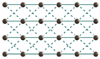
Figure 5: Weighted graph state as a universal resource. Solid lines correspond to edges that have been entangled using phase gates with phase $\phi=\pi$, dotted lines correspond to edges entangled with phase gates with $\phi=\pi/2$. This shows that one can replace some edges with weakly entangled bonds.

IV.3.1 Translationally invariant weighted graph states

Expanding the discussion presented in Ref. [1], we treat the weighted graph state shown in Fig. 5. A tensor network representation of these states can be derived along the same lines as for the original cluster in Section III.3. Set $\mbox{$|i\rangle$}:=2^{-1/2}(\mbox{$|0\rangle$}+i\mbox{$|1\rangle$})$. The relevant tensors are given by

(270)

(277)

Indices are labeled $ru$ for “right-up” to $ld$ for “left-down”. The boundary conditions are $|0\rangle$ for the $ru,lu,r$-directions; $|+\rangle$ otherwise.

We will first describe how to realize isolated evolutions of single logical qubits in the sense of Fig. 1. Again the strategy will be to measure the sites of one horizontal line of the lattice in the $X$-basis and all vertically adjacent systems in the $Z$-basis. The analysis of the situation proceeds in perfect analogy to the one given in Section III.5. One obtains

$$\lx@xy@svg{\hbox{\raise 0.0pt\hbox{\kern 62.76192pt\hbox{{\hbox{\kern-62.76192pt\raise 0.0pt\hbox{\hbox{\kern 0.0pt\raise 16.26666pt\lx@xy@svgnested{\hbox{\raise 0.0pt\hbox{\kern 18.97725pt\hbox{\ignorespaces\ignorespaces\ignorespaces\hbox{\vtop{\kern 0.0pt\offinterlineskip\halign{\entry@#!@&&\entry@@#!@\cr&&\\&&\\&&\\}}}\ignorespaces{{{\hbox{\framed@@{0.0pt}}}}\hbox{\kern-18.97725pt\raise 0.0pt\hbox{\hbox{\kern 3.0pt\raise-2.28223pt\hbox{$\textstyle{A[Z_{i-1,u}]}$}}}}}{\hbox{\kern 39.5402pt\raise 0.0pt\hbox{\hbox{\kern 0.0pt\raise 0.0pt\hbox{\hbox{\kern 3.0pt\raise 0.0pt\hbox{$\textstyle{}$}}}}}}}{{{\hbox{\framed@@{0.0pt}}}}\hbox{\kern 66.10316pt\raise 0.0pt\hbox{\hbox{\kern 3.0pt\raise-2.28223pt\hbox{$\textstyle{A[Z_{i+1,u}]}$}}}}}{\hbox{\kern-3.0pt\raise-16.21777pt\hbox{\hbox{\kern 0.0pt\raise 0.0pt\hbox{\hbox{\kern 3.0pt\raise 0.0pt\hbox{$\textstyle{\ignorespaces\ignorespaces\ignorespaces\ignorespaces}$}}}}}}}\ignorespaces\ignorespaces\ignorespaces\ignorespaces{}{\hbox{\lx@xy@droprule}}\ignorespaces{\hbox{\kern 27.51306pt\raise-16.21777pt\hbox{\hbox{\kern 0.0pt\raise 0.0pt\hbox{\lx@xy@tip{1}\lx@xy@tip{-1}}}}}}{\hbox{\lx@xy@droprule}}{\hbox{\lx@xy@droprule}}{{{\hbox{\framed@@{0.0pt}}}}\hbox{\kern 27.51306pt\raise-16.21777pt\hbox{\hbox{\kern 3.0pt\raise-2.5pt\hbox{$\textstyle{A[X_{i}]}$}}}}}\ignorespaces\ignorespaces\ignorespaces{}\ignorespaces\ignorespaces{\hbox{\lx@xy@drawline@}}\ignorespaces{}\ignorespaces\ignorespaces{\hbox{\lx@xy@drawline@}}\ignorespaces{\hbox{\lx@xy@drawline@}}\ignorespaces\ignorespaces\ignorespaces{}\ignorespaces\ignorespaces{\hbox{\lx@xy@drawline@}}\ignorespaces{}\ignorespaces\ignorespaces{\hbox{\lx@xy@drawline@}}\ignorespaces{\hbox{\lx@xy@drawline@}}\ignorespaces\ignorespaces\ignorespaces\ignorespaces{}{\hbox{\lx@xy@droprule}}\ignorespaces{\hbox{\kern 83.32487pt\raise-16.21777pt\hbox{\hbox{\kern 0.0pt\raise 0.0pt\hbox{\lx@xy@tip{1}\lx@xy@tip{-1}}}}}}{\hbox{\lx@xy@droprule}}{\hbox{\lx@xy@droprule}}{\hbox{\kern 83.32487pt\raise-16.21777pt\hbox{\hbox{\kern 0.0pt\raise 0.0pt\hbox{\hbox{\kern 3.0pt\raise 0.0pt\hbox{$\textstyle{}$}}}}}}}{{{\hbox{\framed@@{0.0pt}}}}\hbox{\kern-18.83173pt\raise-32.48444pt\hbox{\hbox{\kern 3.0pt\raise-2.23334pt\hbox{$\textstyle{A[Z_{i-1,d}]}$}}}}}\ignorespaces\ignorespaces\ignorespaces{}\ignorespaces\ignorespaces{\hbox{\lx@xy@drawline@}}\ignorespaces{}\ignorespaces\ignorespaces{\hbox{\lx@xy@drawline@}}\ignorespaces{\hbox{\lx@xy@drawline@}}{\hbox{\kern 39.5402pt\raise-32.48444pt\hbox{\hbox{\kern 0.0pt\raise 0.0pt\hbox{\hbox{\kern 3.0pt\raise 0.0pt\hbox{$\textstyle{}$}}}}}}}{{{\hbox{\framed@@{0.0pt}}}}\hbox{\kern 66.24869pt\raise-32.48444pt\hbox{\hbox{\kern 3.0pt\raise-2.23334pt\hbox{$\textstyle{A[Z_{i+1,d}]}$}}}}}\ignorespaces\ignorespaces\ignorespaces{}\ignorespaces\ignorespaces{\hbox{\lx@xy@drawline@}}\ignorespaces{}\ignorespaces\ignorespaces{\hbox{\lx@xy@drawline@}}\ignorespaces{\hbox{\lx@xy@drawline@}}\ignorespaces\ignorespaces}}}}}}}}}}}}=HS^{2x_{i}+z_{i}}, \textstyle{A[Z_{i-1,u}]} \textstyle{A[Z_{i+1,u}]} \textstyle{A[X_{i}]} \textstyle{A[Z_{i-1,d}]} \textstyle{A[Z_{i+1,d}]} \textstyle{A[Z_{i-1,u}]} \textstyle{A[Z_{i+1,u}]} \textstyle{A[X_{i}]} \textstyle{A[Z_{i-1,d}]} \textstyle{A[Z_{i+1,d}]}$$ (278)

where

$$z_{i}=z_{i-1,u}+z_{i-1,d}+z_{i+1,u}+z_{i+1,d},$$ (279)

and $S:=\operatorname{diag}(1,i)$ denotes the $\pi/4$ gate.

The operators $H$ and $S$ generate the 24-element single qubit Clifford group. Following the approach of Section IV.1, we take this as the model’s by-product group.

Now choose some phase $\phi$. Re-doing the calculation which led to Eq. (278), where we now measure in the $\{\mbox{$|0\rangle$}\pm e^{i\phi}\mbox{$|1\rangle$}\}$-basis instead of $X$ on the central node, shows that the evolution of the correlation space is given by $S(\phi)$, up to by-products. In complete analogy to Section IV.1, we see that the model allows for the realization of arbitrary $SU(2)$ operations.

How to prepare the state of the correlation system for a single horizontal line and how to read read it out has already been discussed in Section III.3. Hence the only piece missing for universal quantum computation is a single entangling two-qubit gate.

The schematics for a controlled-$Z$ gate between two horizontal lines in the lattice are given below. We implicitly assume that all adjacent sites not shown are measured in the $Z$-basis,

$$\lx@xy@svg{\hbox{\raise 0.0pt\hbox{\kern 76.64023pt\hbox{{\hbox{\kern-76.64023pt\raise 0.0pt\hbox{\hbox{\kern 0.0pt\raise 18.84526pt\lx@xy@svgnested{\hbox{\raise 0.0pt\hbox{\kern 3.0pt\hbox{\ignorespaces\ignorespaces\ignorespaces\hbox{\vtop{\kern 0.0pt\offinterlineskip\halign{\entry@#!@&&\entry@@#!@\cr&&&&\\&&\\&&&&\crcr}}}\ignorespaces{\hbox{\kern-3.0pt\raise 0.0pt\hbox{\hbox{\kern 0.0pt\raise 0.0pt\hbox{\hbox{\kern 3.0pt\raise 0.0pt\hbox{$\textstyle{\ignorespaces\ignorespaces\ignorespaces\ignorespaces}$}}}}}}}\ignorespaces\ignorespaces\ignorespaces\ignorespaces{}{\hbox{\lx@xy@droprule}}\ignorespaces{\hbox{\kern 17.22636pt\raise 0.0pt\hbox{\hbox{\kern 0.0pt\raise 0.0pt\hbox{\lx@xy@tip{1}\lx@xy@tip{-1}}}}}}{\hbox{\lx@xy@droprule}}{\hbox{\lx@xy@droprule}}{{{\hbox{\framed@@{0.0pt}}}}\hbox{\kern 17.22636pt\raise 0.0pt\hbox{\hbox{\kern 3.0pt\raise-2.5pt\hbox{$\textstyle{A[X]}$}}}}}\ignorespaces\ignorespaces\ignorespaces\ignorespaces{}{\hbox{\lx@xy@droprule}}\ignorespaces{}{\hbox{\lx@xy@droprule}}{\hbox{\lx@xy@droprule}}{{{\hbox{\framed@@{0.0pt}}}}\hbox{\kern 59.57773pt\raise 0.0pt\hbox{\hbox{\kern 3.0pt\raise-2.5pt\hbox{$\textstyle{A[X]}$}}}}}\ignorespaces\ignorespaces\ignorespaces\ignorespaces{}{\hbox{\lx@xy@droprule}}\ignorespaces{}{\hbox{\lx@xy@droprule}}{\hbox{\lx@xy@droprule}}{{{\hbox{\framed@@{0.0pt}}}}\hbox{\kern 101.9291pt\raise 0.0pt\hbox{\hbox{\kern 3.0pt\raise-2.5pt\hbox{$\textstyle{A[X]}$}}}}}\ignorespaces\ignorespaces\ignorespaces\ignorespaces{}{\hbox{\lx@xy@droprule}}\ignorespaces{\hbox{\kern 144.28046pt\raise 0.0pt\hbox{\hbox{\kern 0.0pt\raise 0.0pt\hbox{\lx@xy@tip{1}\lx@xy@tip{-1}}}}}}{\hbox{\lx@xy@droprule}}{\hbox{\lx@xy@droprule}}{\hbox{\kern 144.28046pt\raise 0.0pt\hbox{\hbox{\kern 0.0pt\raise 0.0pt\hbox{\hbox{\kern 3.0pt\raise 0.0pt\hbox{$\textstyle{}$}}}}}}}{\hbox{\kern-3.0pt\raise-18.84526pt\hbox{\hbox{\kern 0.0pt\raise 0.0pt\hbox{\hbox{\kern 3.0pt\raise 0.0pt\hbox{$\textstyle{}$}}}}}}}{\hbox{\kern 28.28886pt\raise-18.84526pt\hbox{\hbox{\kern 0.0pt\raise 0.0pt\hbox{\hbox{\kern 3.0pt\raise 0.0pt\hbox{$\textstyle{}$}}}}}}}{{{\hbox{\framed@@{0.0pt}}}}\hbox{\kern 60.09854pt\raise-18.84526pt\hbox{\hbox{\kern 3.0pt\raise-2.5pt\hbox{$\textstyle{A[Y]}$}}}}}\ignorespaces\ignorespaces\ignorespaces{}\ignorespaces\ignorespaces{\hbox{\lx@xy@drawline@}}\ignorespaces{}\ignorespaces\ignorespaces{\hbox{\lx@xy@drawline@}}\ignorespaces{\hbox{\lx@xy@drawline@}}\ignorespaces\ignorespaces\ignorespaces{}\ignorespaces\ignorespaces{\hbox{\lx@xy@drawline@}}\ignorespaces{}\ignorespaces\ignorespaces{\hbox{\lx@xy@drawline@}}\ignorespaces{\hbox{\lx@xy@drawline@}}{\hbox{\kern-3.0pt\raise-37.69052pt\hbox{\hbox{\kern 0.0pt\raise 0.0pt\hbox{\hbox{\kern 3.0pt\raise 0.0pt\hbox{$\textstyle{\ignorespaces\ignorespaces\ignorespaces\ignorespaces}$}}}}}}}\ignorespaces\ignorespaces\ignorespaces\ignorespaces{}{\hbox{\lx@xy@droprule}}\ignorespaces{\hbox{\kern 17.22636pt\raise-37.69052pt\hbox{\hbox{\kern 0.0pt\raise 0.0pt\hbox{\lx@xy@tip{1}\lx@xy@tip{-1}}}}}}{\hbox{\lx@xy@droprule}}{\hbox{\lx@xy@droprule}}{{{\hbox{\framed@@{0.0pt}}}}\hbox{\kern 17.22636pt\raise-37.69052pt\hbox{\hbox{\kern 3.0pt\raise-2.5pt\hbox{$\textstyle{A[X]}$}}}}}\ignorespaces\ignorespaces\ignorespaces\ignorespaces{}{\hbox{\lx@xy@droprule}}\ignorespaces{}{\hbox{\lx@xy@droprule}}{\hbox{\lx@xy@droprule}}\ignorespaces\ignorespaces\ignorespaces{}\ignorespaces\ignorespaces{\hbox{\lx@xy@drawline@}}\ignorespaces{}\ignorespaces\ignorespaces{\hbox{\lx@xy@drawline@}}\ignorespaces{\hbox{\lx@xy@drawline@}}{{{\hbox{\framed@@{0.0pt}}}}\hbox{\kern 59.57773pt\raise-37.69052pt\hbox{\hbox{\kern 3.0pt\raise-2.5pt\hbox{$\textstyle{A[X]}$}}}}}\ignorespaces\ignorespaces\ignorespaces\ignorespaces{}{\hbox{\lx@xy@droprule}}\ignorespaces{}{\hbox{\lx@xy@droprule}}{\hbox{\lx@xy@droprule}}{{{\hbox{\framed@@{0.0pt}}}}\hbox{\kern 101.9291pt\raise-37.69052pt\hbox{\hbox{\kern 3.0pt\raise-2.5pt\hbox{$\textstyle{A[X]}$}}}}}\ignorespaces\ignorespaces\ignorespaces{}\ignorespaces\ignorespaces{\hbox{\lx@xy@drawline@}}\ignorespaces{}\ignorespaces\ignorespaces{\hbox{\lx@xy@drawline@}}\ignorespaces{\hbox{\lx@xy@drawline@}}\ignorespaces\ignorespaces\ignorespaces\ignorespaces{}{\hbox{\lx@xy@droprule}}\ignorespaces{\hbox{\kern 144.28046pt\raise-37.69052pt\hbox{\hbox{\kern 0.0pt\raise 0.0pt\hbox{\lx@xy@tip{1}\lx@xy@tip{-1}}}}}}{\hbox{\lx@xy@droprule}}{\hbox{\lx@xy@droprule}}{\hbox{\kern 144.28046pt\raise-37.69052pt\hbox{\hbox{\kern 0.0pt\raise 0.0pt\hbox{\hbox{\kern 3.0pt\raise 0.0pt\hbox{$\textstyle{}$}}}}}}}\ignorespaces\ignorespaces}}}}}}}}}}}}. \textstyle{A[X]} \textstyle{A[X]} \textstyle{A[X]} \textstyle{A[Y]} \textstyle{A[X]} \textstyle{A[X]} \textstyle{A[X]} \textstyle{A[X]} \textstyle{A[X]} \textstyle{A[X]} \textstyle{A[Y]} \textstyle{A[X]} \textstyle{A[X]} \textstyle{A[X]}$$ (280)

The measurement scheme realizes a controlled-$Z$ gate, where the correlation system of the lower line carries the control qubit and the upper line the target qubit.

In detail one would proceed as follows: first one performs the $X$-measurements on the sites shown and the $Z$-measurements on the adjacent ones. If any of these measurements yields the result “$1$”, we apply a $Z$-measurement to the central site and restart the procedure three sites to the right. This approach has been chosen for convenience: it allows us to forget about possible phases introduced by other measurement outcomes. Still, the “correct” result will occur after a finite expected number of steps, so the overhead caused due to this simplification is only linear. It is also not hard to see that most other outcomes can be compensated for – so for practical purposes the scheme could be vastly optimized.

Now assume that all measurements yielded “$0$”. Then a $Y$-measurement is performed on the central site, obtaining the result $y$. As we did in Section IV.1.4, we assume that the (lower) control line is in the basis state $|c\rangle$, for $c\in\{0,1\}$. The contraction of the lower-most three tensors gives

$$= S^{c}\mbox{$|+\rangle$}_{lu}S^{c}\mbox{$|+\rangle$}_{ru}H\mbox{$|c\rangle$}_{r},$$

where as before $S=S(i)=\operatorname{diag}(1,i)$. We plug this result into the $A[Y]$ tensor:

$$= \mbox{$|+\rangle$}_{lu}\,\mbox{$|+\rangle$}_{ru}+(-1)^{c+y}i(S\otimes S)\mbox{$|+\rangle$}_{lu}\,\mbox{$|+\rangle$}_{ru}.$$

Lastly, for $x\in\{0,1\}$,

$$\lx@xy@svg{\hbox{\raise 0.0pt\hbox{\kern 67.48746pt\hbox{{\hbox{\kern-67.48746pt\raise 0.0pt\hbox{\hbox{\kern 0.0pt\raise 12.53734pt\lx@xy@svgnested{\hbox{\raise 0.0pt\hbox{\kern 3.0pt\hbox{\ignorespaces\ignorespaces\ignorespaces\hbox{\vtop{\kern 0.0pt\offinterlineskip\halign{\entry@#!@&&\entry@@#!@\cr&&&&\\&&&\crcr}}}\ignorespaces{\hbox{\kern-3.0pt\raise 0.0pt\hbox{\hbox{\kern 0.0pt\raise 0.0pt\hbox{\hbox{\kern 3.0pt\raise 0.0pt\hbox{$\textstyle{\ignorespaces\ignorespaces\ignorespaces\ignorespaces}$}}}}}}}\ignorespaces\ignorespaces\ignorespaces\ignorespaces{}{\hbox{\lx@xy@droprule}}\ignorespaces{\hbox{\kern 12.64998pt\raise 0.0pt\hbox{\hbox{\kern 0.0pt\raise 0.0pt\hbox{\lx@xy@tip{1}\lx@xy@tip{-1}}}}}}{\hbox{\lx@xy@droprule}}{\hbox{\lx@xy@droprule}}{{{\hbox{\framed@@{0.0pt}}}}\hbox{\kern 12.64998pt\raise 0.0pt\hbox{\hbox{\kern 3.0pt\raise-2.5pt\hbox{$\textstyle{A[X]}$}}}}}\ignorespaces\ignorespaces\ignorespaces\ignorespaces{}{\hbox{\lx@xy@droprule}}\ignorespaces{}{\hbox{\lx@xy@droprule}}{\hbox{\lx@xy@droprule}}{{{\hbox{\framed@@{0.0pt}}}}\hbox{\kern 50.42496pt\raise 0.0pt\hbox{\hbox{\kern 3.0pt\raise-2.5pt\hbox{$\textstyle{A[X]}$}}}}}\ignorespaces\ignorespaces\ignorespaces\ignorespaces{}{\hbox{\lx@xy@droprule}}\ignorespaces{}{\hbox{\lx@xy@droprule}}{\hbox{\lx@xy@droprule}}{{{\hbox{\framed@@{0.0pt}}}}\hbox{\kern 88.19994pt\raise 0.0pt\hbox{\hbox{\kern 3.0pt\raise-2.5pt\hbox{$\textstyle{A[X]}$}}}}}\ignorespaces\ignorespaces\ignorespaces\ignorespaces{}{\hbox{\lx@xy@droprule}}\ignorespaces{\hbox{\kern 125.97491pt\raise 0.0pt\hbox{\hbox{\kern 0.0pt\raise 0.0pt\hbox{\lx@xy@tip{1}\lx@xy@tip{-1}}}}}}{\hbox{\lx@xy@droprule}}{\hbox{\lx@xy@droprule}}{\hbox{\kern 125.97491pt\raise 0.0pt\hbox{\hbox{\kern 0.0pt\raise 0.0pt\hbox{\hbox{\kern 3.0pt\raise 0.0pt\hbox{$\textstyle{}$}}}}}}}{\hbox{\kern-3.0pt\raise-24.80524pt\hbox{\hbox{\kern 0.0pt\raise 0.0pt\hbox{\hbox{\kern 3.0pt\raise 0.0pt\hbox{$\textstyle{}$}}}}}}}{{{\hbox{\framed@@{0.0pt}}}}\hbox{\kern 11.53581pt\raise-24.80524pt\hbox{\hbox{\kern 3.0pt\raise-2.76944pt\hbox{$\textstyle{S^{x}\mbox{$|+\rangle$}}$}}}}}\ignorespaces\ignorespaces\ignorespaces\ignorespaces{}{\hbox{\lx@xy@droprule}}\ignorespaces{}{\hbox{\lx@xy@droprule}}{\hbox{\lx@xy@droprule}}{\hbox{\kern 61.48746pt\raise-24.80524pt\hbox{\hbox{\kern 0.0pt\raise 0.0pt\hbox{\hbox{\kern 3.0pt\raise 0.0pt\hbox{$\textstyle{}$}}}}}}}{{{\hbox{\framed@@{0.0pt}}}}\hbox{\kern 87.08577pt\raise-24.80524pt\hbox{\hbox{\kern 3.0pt\raise-2.76944pt\hbox{$\textstyle{S^{x}\mbox{$|+\rangle$}}$}}}}}\ignorespaces\ignorespaces\ignorespaces\ignorespaces{}{\hbox{\lx@xy@droprule}}\ignorespaces{}{\hbox{\lx@xy@droprule}}{\hbox{\lx@xy@droprule}}\ignorespaces\ignorespaces}}}}}}}}}}}}=HZ^{x}. \textstyle{A[X]} \textstyle{A[X]} \textstyle{A[X]} \textstyle{S^{x}\mbox{$|+\rangle$}} \textstyle{S^{x}\mbox{$|+\rangle$}} \textstyle{A[X]} \textstyle{A[X]} \textstyle{A[X]} \textstyle{S^{x}\mbox{$|+\rangle$}} \textstyle{S^{x}\mbox{$|+\rangle$}}$$ (297)

Hence, the evolution on the upper line is

$$H(\mathbbm{1}+(-1)^{c+y}iZ)\propto HSZ^{y+c},$$ (298)

equivalent to $Z^{c}$ up to by-products. We arrive hence at the following conclusion:

Observation 7 (Non-maximal entangling power).

Universal resouces may be prepared using commuting gates with non-maximal entangling power.

IV.3.2 Rerouting

we will consider a second weighted graph state to exemplify yet another novel ingredient that one can make use of in measurement-based quantum computation: One can think of quantum information being transported in the correlation system of some systems on the lattice forming “wires”, in a way that gates are realized by bringing the “wires” together. This is an element that is not present in the original one-way computer. The subsequent example of a resource state has not been chosen for its plausibility in the preparation in a physical context, but in a way such that this idea of “rerouting quantum information” can very transparently be explained, see Fig. 6.

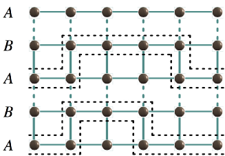
Figure 6: Weighted graph state where the gate is achieved by appropriately bringing two wires together in a “rerouting process”.

The resource that we think about is defined by tensors that are fully translationally invariant in one dimension, and has period two in the orthogonal dimension,

$$\lx@xy@svg{\hbox{\raise 0.0pt\hbox{\kern 83.89607pt\hbox{{\hbox{\kern-83.89607pt\raise 0.0pt\hbox{\hbox{\kern 0.0pt\raise 39.3216pt\lx@xy@svgnested{\hbox{\raise 0.0pt\hbox{\kern 3.0pt\hbox{\ignorespaces\ignorespaces\ignorespaces\hbox{\vtop{\kern 0.0pt\offinterlineskip\halign{\entry@#!@&&\entry@@#!@\cr&&&&&&\\&&&&&&\\&&&&&&\\&&&&&&\\&&&&&&\crcr}}}\ignorespaces{\hbox{\kern-3.0pt\raise 0.0pt\hbox{\hbox{\kern 0.0pt\raise 0.0pt\hbox{\hbox{\kern 3.0pt\raise 0.0pt\hbox{$\textstyle{}$}}}}}}}{\hbox{\kern 21.26976pt\raise 0.0pt\hbox{\hbox{\kern 0.0pt\raise 0.0pt\hbox{\hbox{\kern 3.0pt\raise 0.0pt\hbox{$\textstyle{\ignorespaces\ignorespaces\ignorespaces\ignorespaces}$}}}}}}}\ignorespaces\ignorespaces\ignorespaces\ignorespaces{}{\hbox{\lx@xy@droprule}}\ignorespaces{}{\hbox{\lx@xy@droprule}}{\hbox{\lx@xy@droprule}}{\hbox{\kern 49.58292pt\raise 0.0pt\hbox{\hbox{\kern 0.0pt\raise 0.0pt\hbox{\hbox{\kern 3.0pt\raise 0.0pt\hbox{$\textstyle{\ignorespaces\ignorespaces\ignorespaces\ignorespaces}$}}}}}}}\ignorespaces\ignorespaces\ignorespaces\ignorespaces{}{\hbox{\lx@xy@droprule}}\ignorespaces{}{\hbox{\lx@xy@droprule}}{\hbox{\lx@xy@droprule}}{\hbox{\kern 77.89607pt\raise 0.0pt\hbox{\hbox{\kern 0.0pt\raise 0.0pt\hbox{\hbox{\kern 3.0pt\raise 0.0pt\hbox{$\textstyle{\ignorespaces\ignorespaces\ignorespaces\ignorespaces}$}}}}}}}\ignorespaces\ignorespaces\ignorespaces\ignorespaces{}{\hbox{\lx@xy@droprule}}\ignorespaces{}{\hbox{\lx@xy@droprule}}{\hbox{\lx@xy@droprule}}{\hbox{\kern 106.20923pt\raise 0.0pt\hbox{\hbox{\kern 0.0pt\raise 0.0pt\hbox{\hbox{\kern 3.0pt\raise 0.0pt\hbox{$\textstyle{\ignorespaces\ignorespaces\ignorespaces\ignorespaces}$}}}}}}}\ignorespaces\ignorespaces\ignorespaces\ignorespaces{}{\hbox{\lx@xy@droprule}}\ignorespaces{}{\hbox{\lx@xy@droprule}}{\hbox{\lx@xy@droprule}}{\hbox{\kern 134.52238pt\raise 0.0pt\hbox{\hbox{\kern 0.0pt\raise 0.0pt\hbox{\hbox{\kern 3.0pt\raise 0.0pt\hbox{$\textstyle{\ignorespaces\ignorespaces\ignorespaces\ignorespaces}$}}}}}}}\ignorespaces\ignorespaces\ignorespaces\ignorespaces{}{\hbox{\lx@xy@droprule}}\ignorespaces{}{\hbox{\lx@xy@droprule}}{\hbox{\lx@xy@droprule}}{\hbox{\kern 158.79214pt\raise 0.0pt\hbox{\hbox{\kern 0.0pt\raise 0.0pt\hbox{\hbox{\kern 3.0pt\raise 0.0pt\hbox{$\textstyle{}$}}}}}}}{\hbox{\kern-3.0pt\raise-17.95247pt\hbox{\hbox{\kern 0.0pt\raise 0.0pt\hbox{\hbox{\kern 3.0pt\raise 0.0pt\hbox{$\textstyle{\ignorespaces\ignorespaces\ignorespaces\ignorespaces}$}}}}}}}\ignorespaces\ignorespaces\ignorespaces\ignorespaces{}{\hbox{\lx@xy@droprule}}\ignorespaces{}{\hbox{\lx@xy@droprule}}{\hbox{\lx@xy@droprule}}{{{\hbox{\framed@@{0.0pt}}}}\hbox{\kern 17.51976pt\raise-17.95247pt\hbox{\hbox{\kern 3.0pt\raise-3.41666pt\hbox{$\textstyle{A}$}}}}}\ignorespaces\ignorespaces\ignorespaces\ignorespaces{}{\hbox{\lx@xy@droprule}}\ignorespaces{}{\hbox{\lx@xy@droprule}}{\hbox{\lx@xy@droprule}}{{{\hbox{\framed@@{0.0pt}}}}\hbox{\kern 45.83292pt\raise-17.95247pt\hbox{\hbox{\kern 3.0pt\raise-3.41666pt\hbox{$\textstyle{A}$}}}}}\ignorespaces\ignorespaces\ignorespaces\ignorespaces{}{\hbox{\lx@xy@droprule}}\ignorespaces{}{\hbox{\lx@xy@droprule}}{\hbox{\lx@xy@droprule}}{{{\hbox{\framed@@{0.0pt}}}}\hbox{\kern 74.14607pt\raise-17.95247pt\hbox{\hbox{\kern 3.0pt\raise-3.41666pt\hbox{$\textstyle{A}$}}}}}\ignorespaces\ignorespaces\ignorespaces\ignorespaces{}{\hbox{\lx@xy@droprule}}\ignorespaces{}{\hbox{\lx@xy@droprule}}{\hbox{\lx@xy@droprule}}{{{\hbox{\framed@@{0.0pt}}}}\hbox{\kern 102.45923pt\raise-17.95247pt\hbox{\hbox{\kern 3.0pt\raise-3.41666pt\hbox{$\textstyle{A}$}}}}}\ignorespaces\ignorespaces\ignorespaces\ignorespaces{}{\hbox{\lx@xy@droprule}}\ignorespaces{}{\hbox{\lx@xy@droprule}}{\hbox{\lx@xy@droprule}}{{{\hbox{\framed@@{0.0pt}}}}\hbox{\kern 130.77238pt\raise-17.95247pt\hbox{\hbox{\kern 3.0pt\raise-3.41666pt\hbox{$\textstyle{A}$}}}}}\ignorespaces\ignorespaces\ignorespaces\ignorespaces{}{\hbox{\lx@xy@droprule}}\ignorespaces{}{\hbox{\lx@xy@droprule}}{\hbox{\lx@xy@droprule}}{\hbox{\kern 158.79214pt\raise-17.95247pt\hbox{\hbox{\kern 0.0pt\raise 0.0pt\hbox{\hbox{\kern 3.0pt\raise 0.0pt\hbox{$\textstyle{}$}}}}}}}{\hbox{\kern-3.0pt\raise-39.3216pt\hbox{\hbox{\kern 0.0pt\raise 0.0pt\hbox{\hbox{\kern 3.0pt\raise 0.0pt\hbox{$\textstyle{\ignorespaces\ignorespaces\ignorespaces\ignorespaces}$}}}}}}}\ignorespaces\ignorespaces\ignorespaces\ignorespaces{}{\hbox{\lx@xy@droprule}}\ignorespaces{}{\hbox{\lx@xy@droprule}}{\hbox{\lx@xy@droprule}}{{{\hbox{\framed@@{0.0pt}}}}\hbox{\kern 17.22636pt\raise-39.3216pt\hbox{\hbox{\kern 3.0pt\raise-3.41666pt\hbox{$\textstyle{B}$}}}}}\ignorespaces\ignorespaces\ignorespaces\ignorespaces{}{\hbox{\lx@xy@droprule}}\ignorespaces{}{\hbox{\lx@xy@droprule}}{\hbox{\lx@xy@droprule}}\ignorespaces\ignorespaces\ignorespaces\ignorespaces{}{\hbox{\lx@xy@droprule}}\ignorespaces{}{\hbox{\lx@xy@droprule}}{\hbox{\lx@xy@droprule}}\ignorespaces\ignorespaces\ignorespaces\ignorespaces{}{\hbox{\lx@xy@droprule}}\ignorespaces{}{\hbox{\lx@xy@droprule}}{\hbox{\lx@xy@droprule}}{{{\hbox{\framed@@{0.0pt}}}}\hbox{\kern 45.53952pt\raise-39.3216pt\hbox{\hbox{\kern 3.0pt\raise-3.41666pt\hbox{$\textstyle{B}$}}}}}\ignorespaces\ignorespaces\ignorespaces\ignorespaces{}{\hbox{\lx@xy@droprule}}\ignorespaces{}{\hbox{\lx@xy@droprule}}{\hbox{\lx@xy@droprule}}\ignorespaces\ignorespaces\ignorespaces\ignorespaces{}{\hbox{\lx@xy@droprule}}\ignorespaces{}{\hbox{\lx@xy@droprule}}{\hbox{\lx@xy@droprule}}\ignorespaces\ignorespaces\ignorespaces\ignorespaces{}{\hbox{\lx@xy@droprule}}\ignorespaces{}{\hbox{\lx@xy@droprule}}{\hbox{\lx@xy@droprule}}{{{\hbox{\framed@@{0.0pt}}}}\hbox{\kern 73.85268pt\raise-39.3216pt\hbox{\hbox{\kern 3.0pt\raise-3.41666pt\hbox{$\textstyle{B}$}}}}}\ignorespaces\ignorespaces\ignorespaces\ignorespaces{}{\hbox{\lx@xy@droprule}}\ignorespaces{}{\hbox{\lx@xy@droprule}}{\hbox{\lx@xy@droprule}}\ignorespaces\ignorespaces\ignorespaces\ignorespaces{}{\hbox{\lx@xy@droprule}}\ignorespaces{}{\hbox{\lx@xy@droprule}}{\hbox{\lx@xy@droprule}}\ignorespaces\ignorespaces\ignorespaces\ignorespaces{}{\hbox{\lx@xy@droprule}}\ignorespaces{}{\hbox{\lx@xy@droprule}}{\hbox{\lx@xy@droprule}}{{{\hbox{\framed@@{0.0pt}}}}\hbox{\kern 102.16583pt\raise-39.3216pt\hbox{\hbox{\kern 3.0pt\raise-3.41666pt\hbox{$\textstyle{B}$}}}}}\ignorespaces\ignorespaces\ignorespaces\ignorespaces{}{\hbox{\lx@xy@droprule}}\ignorespaces{}{\hbox{\lx@xy@droprule}}{\hbox{\lx@xy@droprule}}\ignorespaces\ignorespaces\ignorespaces\ignorespaces{}{\hbox{\lx@xy@droprule}}\ignorespaces{}{\hbox{\lx@xy@droprule}}{\hbox{\lx@xy@droprule}}\ignorespaces\ignorespaces\ignorespaces\ignorespaces{}{\hbox{\lx@xy@droprule}}\ignorespaces{}{\hbox{\lx@xy@droprule}}{\hbox{\lx@xy@droprule}}{{{\hbox{\framed@@{0.0pt}}}}\hbox{\kern 130.47899pt\raise-39.3216pt\hbox{\hbox{\kern 3.0pt\raise-3.41666pt\hbox{$\textstyle{B}$}}}}}\ignorespaces\ignorespaces\ignorespaces\ignorespaces{}{\hbox{\lx@xy@droprule}}\ignorespaces{}{\hbox{\lx@xy@droprule}}{\hbox{\lx@xy@droprule}}\ignorespaces\ignorespaces\ignorespaces\ignorespaces{}{\hbox{\lx@xy@droprule}}\ignorespaces{}{\hbox{\lx@xy@droprule}}{\hbox{\lx@xy@droprule}}\ignorespaces\ignorespaces\ignorespaces\ignorespaces{}{\hbox{\lx@xy@droprule}}\ignorespaces{}{\hbox{\lx@xy@droprule}}{\hbox{\lx@xy@droprule}}{\hbox{\kern 158.79214pt\raise-39.3216pt\hbox{\hbox{\kern 0.0pt\raise 0.0pt\hbox{\hbox{\kern 3.0pt\raise 0.0pt\hbox{$\textstyle{}$}}}}}}}{\hbox{\kern-3.0pt\raise-60.69072pt\hbox{\hbox{\kern 0.0pt\raise 0.0pt\hbox{\hbox{\kern 3.0pt\raise 0.0pt\hbox{$\textstyle{\ignorespaces\ignorespaces\ignorespaces\ignorespaces}$}}}}}}}\ignorespaces\ignorespaces\ignorespaces\ignorespaces{}{\hbox{\lx@xy@droprule}}\ignorespaces{}{\hbox{\lx@xy@droprule}}{\hbox{\lx@xy@droprule}}{{{\hbox{\framed@@{0.0pt}}}}\hbox{\kern 17.51976pt\raise-60.69072pt\hbox{\hbox{\kern 3.0pt\raise-3.41666pt\hbox{$\textstyle{A}$}}}}}\ignorespaces\ignorespaces\ignorespaces\ignorespaces{}{\hbox{\lx@xy@droprule}}\ignorespaces{}{\hbox{\lx@xy@droprule}}{\hbox{\lx@xy@droprule}}\ignorespaces\ignorespaces\ignorespaces\ignorespaces{}{\hbox{\lx@xy@droprule}}\ignorespaces{}{\hbox{\lx@xy@droprule}}{\hbox{\lx@xy@droprule}}{{{\hbox{\framed@@{0.0pt}}}}\hbox{\kern 45.83292pt\raise-60.69072pt\hbox{\hbox{\kern 3.0pt\raise-3.41666pt\hbox{$\textstyle{A}$}}}}}\ignorespaces\ignorespaces\ignorespaces\ignorespaces{}{\hbox{\lx@xy@droprule}}\ignorespaces{}{\hbox{\lx@xy@droprule}}{\hbox{\lx@xy@droprule}}\ignorespaces\ignorespaces\ignorespaces\ignorespaces{}{\hbox{\lx@xy@droprule}}\ignorespaces{}{\hbox{\lx@xy@droprule}}{\hbox{\lx@xy@droprule}}{{{\hbox{\framed@@{0.0pt}}}}\hbox{\kern 74.14607pt\raise-60.69072pt\hbox{\hbox{\kern 3.0pt\raise-3.41666pt\hbox{$\textstyle{A}$}}}}}\ignorespaces\ignorespaces\ignorespaces\ignorespaces{}{\hbox{\lx@xy@droprule}}\ignorespaces{}{\hbox{\lx@xy@droprule}}{\hbox{\lx@xy@droprule}}\ignorespaces\ignorespaces\ignorespaces\ignorespaces{}{\hbox{\lx@xy@droprule}}\ignorespaces{}{\hbox{\lx@xy@droprule}}{\hbox{\lx@xy@droprule}}{{{\hbox{\framed@@{0.0pt}}}}\hbox{\kern 102.45923pt\raise-60.69072pt\hbox{\hbox{\kern 3.0pt\raise-3.41666pt\hbox{$\textstyle{A}$}}}}}\ignorespaces\ignorespaces\ignorespaces\ignorespaces{}{\hbox{\lx@xy@droprule}}\ignorespaces{}{\hbox{\lx@xy@droprule}}{\hbox{\lx@xy@droprule}}\ignorespaces\ignorespaces\ignorespaces\ignorespaces{}{\hbox{\lx@xy@droprule}}\ignorespaces{}{\hbox{\lx@xy@droprule}}{\hbox{\lx@xy@droprule}}{{{\hbox{\framed@@{0.0pt}}}}\hbox{\kern 130.77238pt\raise-60.69072pt\hbox{\hbox{\kern 3.0pt\raise-3.41666pt\hbox{$\textstyle{A}$}}}}}\ignorespaces\ignorespaces\ignorespaces\ignorespaces{}{\hbox{\lx@xy@droprule}}\ignorespaces{}{\hbox{\lx@xy@droprule}}{\hbox{\lx@xy@droprule}}\ignorespaces\ignorespaces\ignorespaces\ignorespaces{}{\hbox{\lx@xy@droprule}}\ignorespaces{}{\hbox{\lx@xy@droprule}}{\hbox{\lx@xy@droprule}}{\hbox{\kern 158.79214pt\raise-60.69072pt\hbox{\hbox{\kern 0.0pt\raise 0.0pt\hbox{\hbox{\kern 3.0pt\raise 0.0pt\hbox{$\textstyle{}$}}}}}}}{\hbox{\kern-3.0pt\raise-78.64319pt\hbox{\hbox{\kern 0.0pt\raise 0.0pt\hbox{\hbox{\kern 3.0pt\raise 0.0pt\hbox{$\textstyle{}$}}}}}}}{\hbox{\kern 21.26976pt\raise-78.64319pt\hbox{\hbox{\kern 0.0pt\raise 0.0pt\hbox{\hbox{\kern 3.0pt\raise 0.0pt\hbox{$\textstyle{}$}}}}}}}{\hbox{\kern 49.58292pt\raise-78.64319pt\hbox{\hbox{\kern 0.0pt\raise 0.0pt\hbox{\hbox{\kern 3.0pt\raise 0.0pt\hbox{$\textstyle{}$}}}}}}}{\hbox{\kern 77.89607pt\raise-78.64319pt\hbox{\hbox{\kern 0.0pt\raise 0.0pt\hbox{\hbox{\kern 3.0pt\raise 0.0pt\hbox{$\textstyle{}$}}}}}}}{\hbox{\kern 106.20923pt\raise-78.64319pt\hbox{\hbox{\kern 0.0pt\raise 0.0pt\hbox{\hbox{\kern 3.0pt\raise 0.0pt\hbox{$\textstyle{}$}}}}}}}{\hbox{\kern 134.52238pt\raise-78.64319pt\hbox{\hbox{\kern 0.0pt\raise 0.0pt\hbox{\hbox{\kern 3.0pt\raise 0.0pt\hbox{$\textstyle{}$}}}}}}}{\hbox{\kern 158.79214pt\raise-78.64319pt\hbox{\hbox{\kern 0.0pt\raise 0.0pt\hbox{\hbox{\kern 3.0pt\raise 0.0pt\hbox{$\textstyle{}$}}}}}}}\ignorespaces\ignorespaces}}}}}}}}}}}}. \textstyle{A} \textstyle{A} \textstyle{A} \textstyle{A} \textstyle{A} \textstyle{B} \textstyle{B} \textstyle{B} \textstyle{B} \textstyle{B} \textstyle{A} \textstyle{A} \textstyle{A} \textstyle{A} \textstyle{A} \textstyle{A} \textstyle{A} \textstyle{A} \textstyle{A} \textstyle{A} \textstyle{B} \textstyle{B} \textstyle{B} \textstyle{B} \textstyle{B} \textstyle{A} \textstyle{A} \textstyle{A} \textstyle{A} \textstyle{A}$$ (299)

This is, we have two kinds of tensors: One set is given by

$$\lx@xy@svg{\hbox{\raise 0.0pt\hbox{\kern 26.85701pt\hbox{{\hbox{\kern-26.85701pt\raise 0.0pt\hbox{\hbox{\kern 0.0pt\raise 19.53581pt\lx@xy@svgnested{\hbox{\raise 0.0pt\hbox{\kern 3.0pt\hbox{\ignorespaces\ignorespaces\ignorespaces\hbox{\vtop{\kern 0.0pt\offinterlineskip\halign{\entry@#!@&&\entry@@#!@\cr&&\\&&\\&&\crcr}}}\ignorespaces{\hbox{\kern-3.0pt\raise 0.0pt\hbox{\hbox{\kern 0.0pt\raise 0.0pt\hbox{\hbox{\kern 3.0pt\raise 0.0pt\hbox{$\textstyle{}$}}}}}}}{\hbox{\kern 20.85701pt\raise 0.0pt\hbox{\hbox{\kern 0.0pt\raise 0.0pt\hbox{\hbox{\kern 3.0pt\raise 0.0pt\hbox{$\textstyle{}$}}}}}}}{\hbox{\kern 44.71402pt\raise 0.0pt\hbox{\hbox{\kern 0.0pt\raise 0.0pt\hbox{\hbox{\kern 3.0pt\raise 0.0pt\hbox{$\textstyle{}$}}}}}}}{\hbox{\kern-3.0pt\raise-19.53581pt\hbox{\hbox{\kern 0.0pt\raise 0.0pt\hbox{\hbox{\kern 3.0pt\raise 0.0pt\hbox{$\textstyle{\ignorespaces\ignorespaces\ignorespaces\ignorespaces}$}}}}}}}\ignorespaces\ignorespaces\ignorespaces\ignorespaces{}{\hbox{\lx@xy@droprule}}\ignorespaces{\hbox{\kern 11.53581pt\raise-19.53581pt\hbox{\hbox{\kern 0.0pt\raise 0.0pt\hbox{\lx@xy@tip{1}\lx@xy@tip{-1}}}}}}{\hbox{\lx@xy@droprule}}{\hbox{\lx@xy@droprule}}{{{\hbox{\framed@@{0.0pt}}}}\hbox{\kern 11.53581pt\raise-19.53581pt\hbox{\hbox{\kern 3.0pt\raise-2.5pt\hbox{$\textstyle{B[0]}$}}}}}\ignorespaces\ignorespaces\ignorespaces\ignorespaces{}{\hbox{\lx@xy@droprule}}\ignorespaces{\hbox{\kern 23.85701pt\raise-3.0pt\hbox{\hbox{\kern 0.0pt\raise 0.0pt\hbox{\lx@xy@tip{1}\lx@xy@tip{-1}}}}}}{\hbox{\lx@xy@droprule}}{\hbox{\lx@xy@droprule}}\ignorespaces\ignorespaces\ignorespaces\ignorespaces{}{\hbox{\lx@xy@droprule}}\ignorespaces{\hbox{\kern 44.71402pt\raise-19.53581pt\hbox{\hbox{\kern 0.0pt\raise 0.0pt\hbox{\lx@xy@tip{1}\lx@xy@tip{-1}}}}}}{\hbox{\lx@xy@droprule}}{\hbox{\lx@xy@droprule}}{\hbox{\kern 44.71402pt\raise-19.53581pt\hbox{\hbox{\kern 0.0pt\raise 0.0pt\hbox{\hbox{\kern 3.0pt\raise 0.0pt\hbox{$\textstyle{}$}}}}}}}{\hbox{\kern-3.0pt\raise-39.07162pt\hbox{\hbox{\kern 0.0pt\raise 0.0pt\hbox{\hbox{\kern 3.0pt\raise 0.0pt\hbox{$\textstyle{}$}}}}}}}{\hbox{\kern 20.85701pt\raise-39.07162pt\hbox{\hbox{\kern 0.0pt\raise 0.0pt\hbox{\hbox{\kern 3.0pt\raise 0.0pt\hbox{$\textstyle{\ignorespaces\ignorespaces\ignorespaces\ignorespaces}$}}}}}}}\ignorespaces\ignorespaces\ignorespaces\ignorespaces{}{\hbox{\lx@xy@droprule}}\ignorespaces{\hbox{\kern 23.85701pt\raise-27.53581pt\hbox{\hbox{\kern 0.0pt\raise 0.0pt\hbox{\lx@xy@tip{1}\lx@xy@tip{-1}}}}}}{\hbox{\lx@xy@droprule}}{\hbox{\lx@xy@droprule}}{\hbox{\kern 44.71402pt\raise-39.07162pt\hbox{\hbox{\kern 0.0pt\raise 0.0pt\hbox{\hbox{\kern 3.0pt\raise 0.0pt\hbox{$\textstyle{}$}}}}}}}\ignorespaces\ignorespaces}}}}}}}}}}}}=\mbox{$|+\rangle$}_{r}\mbox{$|+\rangle$}_{u}\,\mbox{$\langle 0|$}_{l}\mbox{$\langle 0|$}_{d}, \textstyle{B[0]} \textstyle{B[0]}$$ (306)

$$\lx@xy@svg{\hbox{\raise 0.0pt\hbox{\kern 29.35701pt\hbox{{\hbox{\kern-29.35701pt\raise 0.0pt\hbox{\hbox{\kern 0.0pt\raise 19.53581pt\lx@xy@svgnested{\hbox{\raise 0.0pt\hbox{\kern 3.0pt\hbox{\ignorespaces\ignorespaces\ignorespaces\hbox{\vtop{\kern 0.0pt\offinterlineskip\halign{\entry@#!@&&\entry@@#!@\cr&&\\&&\\&&\crcr}}}\ignorespaces{\hbox{\kern-3.0pt\raise 0.0pt\hbox{\hbox{\kern 0.0pt\raise 0.0pt\hbox{\hbox{\kern 3.0pt\raise 0.0pt\hbox{$\textstyle{}$}}}}}}}{\hbox{\kern 20.85701pt\raise 0.0pt\hbox{\hbox{\kern 0.0pt\raise 0.0pt\hbox{\hbox{\kern 3.0pt\raise 0.0pt\hbox{$\textstyle{}$}}}}}}}{\hbox{\kern 47.21402pt\raise 0.0pt\hbox{\hbox{\kern 0.0pt\raise 0.0pt\hbox{\hbox{\kern 3.0pt\raise 0.0pt\hbox{$\textstyle{}$}}}}}}}{\hbox{\kern-3.0pt\raise-19.53581pt\hbox{\hbox{\kern 0.0pt\raise 0.0pt\hbox{\hbox{\kern 3.0pt\raise 0.0pt\hbox{$\textstyle{\ignorespaces\ignorespaces\ignorespaces\ignorespaces}$}}}}}}}\ignorespaces\ignorespaces\ignorespaces\ignorespaces{}{\hbox{\lx@xy@droprule}}\ignorespaces{\hbox{\kern 11.53581pt\raise-19.53581pt\hbox{\hbox{\kern 0.0pt\raise 0.0pt\hbox{\lx@xy@tip{1}\lx@xy@tip{-1}}}}}}{\hbox{\lx@xy@droprule}}{\hbox{\lx@xy@droprule}}{{{\hbox{\framed@@{0.0pt}}}}\hbox{\kern 11.53581pt\raise-19.53581pt\hbox{\hbox{\kern 3.0pt\raise-2.5pt\hbox{$\textstyle{B[1]}$}}}}}\ignorespaces\ignorespaces\ignorespaces\ignorespaces{}{\hbox{\lx@xy@droprule}}\ignorespaces{\hbox{\kern 23.85701pt\raise-3.0pt\hbox{\hbox{\kern 0.0pt\raise 0.0pt\hbox{\lx@xy@tip{1}\lx@xy@tip{-1}}}}}}{\hbox{\lx@xy@droprule}}{\hbox{\lx@xy@droprule}}\ignorespaces\ignorespaces\ignorespaces\ignorespaces{}{\hbox{\lx@xy@droprule}}\ignorespaces{\hbox{\kern 47.21402pt\raise-19.53581pt\hbox{\hbox{\kern 0.0pt\raise 0.0pt\hbox{\lx@xy@tip{1}\lx@xy@tip{-1}}}}}}{\hbox{\lx@xy@droprule}}{\hbox{\lx@xy@droprule}}{\hbox{\kern 47.21402pt\raise-19.53581pt\hbox{\hbox{\kern 0.0pt\raise 0.0pt\hbox{\hbox{\kern 3.0pt\raise 0.0pt\hbox{$\textstyle{}$}}}}}}}{\hbox{\kern-3.0pt\raise-39.07162pt\hbox{\hbox{\kern 0.0pt\raise 0.0pt\hbox{\hbox{\kern 3.0pt\raise 0.0pt\hbox{$\textstyle{}$}}}}}}}{\hbox{\kern 20.85701pt\raise-39.07162pt\hbox{\hbox{\kern 0.0pt\raise 0.0pt\hbox{\hbox{\kern 3.0pt\raise 0.0pt\hbox{$\textstyle{\ignorespaces\ignorespaces\ignorespaces\ignorespaces}$}}}}}}}\ignorespaces\ignorespaces\ignorespaces\ignorespaces{}{\hbox{\lx@xy@droprule}}\ignorespaces{\hbox{\kern 23.85701pt\raise-27.53581pt\hbox{\hbox{\kern 0.0pt\raise 0.0pt\hbox{\lx@xy@tip{1}\lx@xy@tip{-1}}}}}}{\hbox{\lx@xy@droprule}}{\hbox{\lx@xy@droprule}}{\hbox{\kern 44.71402pt\raise-39.07162pt\hbox{\hbox{\kern 0.0pt\raise 0.0pt\hbox{\hbox{\kern 3.0pt\raise 0.0pt\hbox{$\textstyle{\ }$}}}}}}}\ignorespaces\ignorespaces}}}}}}}}}}}}=\mbox{$|-\rangle$}_{r}\mbox{$|i\rangle$}_{u}\,\mbox{$\langle 1|$}_{l}\mbox{$\langle 1|$}_{d} \textstyle{B[1]} \textstyle{B[1]}$$ (313)

whereas the other one is nothing but the familiar one for a 2-D cluster state as in Eqs. (306, 313), with boundary conditions

$$\mbox{$|L\rangle$}=\mbox{$|D\rangle$}=\mbox{$|+\rangle$},\qquad\mbox{$|R\rangle$}=\mbox{$|U\rangle$}=\mbox{$|1\rangle$}.$$ (314)

The resulting state is hence again a weighted graph state, where in one dimension every second edge is replaced by an edge prepared using a gate with non-maximal entangling power. Then, it is not difficult to see that, again with $x,z_{r},z_{u},z_{d},z_{l}\in\{0,1\}$,

$$\lx@xy@svg{\hbox{\raise 0.0pt\hbox{\kern 36.70523pt\hbox{{\hbox{\kern-36.70523pt\raise 0.0pt\hbox{\hbox{\kern 0.0pt\raise 36.80371pt\lx@xy@svgnested{\hbox{\raise 0.0pt\hbox{\kern 3.0pt\hbox{\ignorespaces\ignorespaces\ignorespaces\hbox{\vtop{\kern 0.0pt\offinterlineskip\halign{\entry@#!@&&\entry@@#!@\cr&&&\\&\\&&\\&\\}}}\ignorespaces{\hbox{\kern-3.0pt\raise 0.0pt\hbox{\hbox{\kern 0.0pt\raise 0.0pt\hbox{\hbox{\kern 3.0pt\raise 0.0pt\hbox{$\textstyle{}$}}}}}}}{\hbox{\kern 23.43732pt\raise 0.0pt\hbox{\hbox{\kern 0.0pt\raise 0.0pt\hbox{\hbox{\kern 3.0pt\raise 0.0pt\hbox{$\textstyle{}$}}}}}}}{\hbox{\kern 49.87463pt\raise 0.0pt\hbox{\hbox{\kern 0.0pt\raise 0.0pt\hbox{\hbox{\kern 3.0pt\raise 0.0pt\hbox{$\textstyle{}$}}}}}}}{\hbox{\kern 64.41045pt\raise 0.0pt\hbox{\hbox{\kern 0.0pt\raise 0.0pt\hbox{\hbox{\kern 3.0pt\raise 0.0pt\hbox{$\textstyle{}$}}}}}}}{\hbox{\kern-3.0pt\raise-19.53581pt\hbox{\hbox{\kern 0.0pt\raise 0.0pt\hbox{\hbox{\kern 3.0pt\raise 0.0pt\hbox{$\textstyle{}$}}}}}}}{{{\hbox{\framed@@{0.0pt}}}}\hbox{\kern 11.53581pt\raise-19.53581pt\hbox{\hbox{\kern 3.0pt\raise-2.5pt\hbox{$\textstyle{A[Z_{u}]}$}}}}}{\hbox{\kern-3.0pt\raise-44.07162pt\hbox{\hbox{\kern 0.0pt\raise 0.0pt\hbox{\hbox{\kern 3.0pt\raise 0.0pt\hbox{$\textstyle{\ignorespaces\ignorespaces\ignorespaces\ignorespaces}$}}}}}}}\ignorespaces\ignorespaces\ignorespaces\ignorespaces{}{\hbox{\lx@xy@droprule}}\ignorespaces{\hbox{\kern 12.08142pt\raise-44.07162pt\hbox{\hbox{\kern 0.0pt\raise 0.0pt\hbox{\lx@xy@tip{1}\lx@xy@tip{-1}}}}}}{\hbox{\lx@xy@droprule}}{\hbox{\lx@xy@droprule}}{{{\hbox{\framed@@{0.0pt}}}}\hbox{\kern 12.08142pt\raise-44.07162pt\hbox{\hbox{\kern 3.0pt\raise-2.5pt\hbox{$\textstyle{B[X]}$}}}}}\ignorespaces\ignorespaces\ignorespaces\ignorespaces{}{\hbox{\lx@xy@droprule}}\ignorespaces{}{\hbox{\lx@xy@droprule}}{\hbox{\lx@xy@droprule}}\ignorespaces\ignorespaces\ignorespaces\ignorespaces{}{\hbox{\lx@xy@droprule}}\ignorespaces{\hbox{\kern 49.87463pt\raise-44.07162pt\hbox{\hbox{\kern 0.0pt\raise 0.0pt\hbox{\lx@xy@tip{1}\lx@xy@tip{-1}}}}}}{\hbox{\lx@xy@droprule}}{\hbox{\lx@xy@droprule}}{\hbox{\kern 49.87463pt\raise-44.07162pt\hbox{\hbox{\kern 0.0pt\raise 0.0pt\hbox{\hbox{\kern 3.0pt\raise 0.0pt\hbox{$\textstyle{}$}}}}}}}{\hbox{\kern-3.0pt\raise-68.60744pt\hbox{\hbox{\kern 0.0pt\raise 0.0pt\hbox{\hbox{\kern 3.0pt\raise 0.0pt\hbox{$\textstyle{}$}}}}}}}{{{\hbox{\framed@@{0.0pt}}}}\hbox{\kern 11.68134pt\raise-68.60744pt\hbox{\hbox{\kern 3.0pt\raise-2.5pt\hbox{$\textstyle{A[Z_{d}]}$}}}}}\ignorespaces\ignorespaces\ignorespaces\ignorespaces{}{\hbox{\lx@xy@droprule}}\ignorespaces{}{\hbox{\lx@xy@droprule}}{\hbox{\lx@xy@droprule}}\ignorespaces\ignorespaces}}}}}}}}}}}}=HZ^{x+z_{d}}S^{z_{u}}, \textstyle{A[Z_{u}]} \textstyle{B[X]} \textstyle{A[Z_{d}]} \textstyle{A[Z_{u}]} \textstyle{B[X]} \textstyle{A[Z_{d}]}$$ (315)

and

$$\lx@xy@svg{\hbox{\raise 0.0pt\hbox{\kern 36.99861pt\hbox{{\hbox{\kern-36.99861pt\raise 0.0pt\hbox{\hbox{\kern 0.0pt\raise 44.07162pt\lx@xy@svgnested{\hbox{\raise 0.0pt\hbox{\kern 3.0pt\hbox{\ignorespaces\ignorespaces\ignorespaces\hbox{\vtop{\kern 0.0pt\offinterlineskip\halign{\entry@#!@&&\entry@@#!@\cr&&&\\&\\&&\\&\\&&\crcr}}}\ignorespaces{\hbox{\kern-3.0pt\raise 0.0pt\hbox{\hbox{\kern 0.0pt\raise 0.0pt\hbox{\hbox{\kern 3.0pt\raise 0.0pt\hbox{$\textstyle{}$}}}}}}}{\hbox{\kern 23.73071pt\raise 0.0pt\hbox{\hbox{\kern 0.0pt\raise 0.0pt\hbox{\hbox{\kern 3.0pt\raise 0.0pt\hbox{$\textstyle{}$}}}}}}}{\hbox{\kern 50.46143pt\raise 0.0pt\hbox{\hbox{\kern 0.0pt\raise 0.0pt\hbox{\hbox{\kern 3.0pt\raise 0.0pt\hbox{$\textstyle{}$}}}}}}}{\hbox{\kern 64.99724pt\raise 0.0pt\hbox{\hbox{\kern 0.0pt\raise 0.0pt\hbox{\hbox{\kern 3.0pt\raise 0.0pt\hbox{$\textstyle{}$}}}}}}}{\hbox{\kern-3.0pt\raise-19.53581pt\hbox{\hbox{\kern 0.0pt\raise 0.0pt\hbox{\hbox{\kern 3.0pt\raise 0.0pt\hbox{$\textstyle{}$}}}}}}}{{{\hbox{\framed@@{0.0pt}}}}\hbox{\kern 11.53581pt\raise-19.53581pt\hbox{\hbox{\kern 3.0pt\raise-2.5pt\hbox{$\textstyle{B[Z_{u}]}$}}}}}{\hbox{\kern-3.0pt\raise-44.07162pt\hbox{\hbox{\kern 0.0pt\raise 0.0pt\hbox{\hbox{\kern 3.0pt\raise 0.0pt\hbox{$\textstyle{\ignorespaces\ignorespaces\ignorespaces\ignorespaces}$}}}}}}}\ignorespaces\ignorespaces\ignorespaces\ignorespaces{}{\hbox{\lx@xy@droprule}}\ignorespaces{\hbox{\kern 12.66821pt\raise-44.07162pt\hbox{\hbox{\kern 0.0pt\raise 0.0pt\hbox{\lx@xy@tip{1}\lx@xy@tip{-1}}}}}}{\hbox{\lx@xy@droprule}}{\hbox{\lx@xy@droprule}}{{{\hbox{\framed@@{0.0pt}}}}\hbox{\kern 12.66821pt\raise-44.07162pt\hbox{\hbox{\kern 3.0pt\raise-2.5pt\hbox{$\textstyle{A[X]}$}}}}}\ignorespaces\ignorespaces\ignorespaces\ignorespaces{}{\hbox{\lx@xy@droprule}}\ignorespaces{}{\hbox{\lx@xy@droprule}}{\hbox{\lx@xy@droprule}}\ignorespaces\ignorespaces\ignorespaces\ignorespaces{}{\hbox{\lx@xy@droprule}}\ignorespaces{\hbox{\kern 50.46143pt\raise-44.07162pt\hbox{\hbox{\kern 0.0pt\raise 0.0pt\hbox{\lx@xy@tip{1}\lx@xy@tip{-1}}}}}}{\hbox{\lx@xy@droprule}}{\hbox{\lx@xy@droprule}}{\hbox{\kern 50.46143pt\raise-44.07162pt\hbox{\hbox{\kern 0.0pt\raise 0.0pt\hbox{\hbox{\kern 3.0pt\raise 0.0pt\hbox{$\textstyle{}$}}}}}}}{\hbox{\kern-3.0pt\raise-68.60744pt\hbox{\hbox{\kern 0.0pt\raise 0.0pt\hbox{\hbox{\kern 3.0pt\raise 0.0pt\hbox{$\textstyle{}$}}}}}}}{{{\hbox{\framed@@{0.0pt}}}}\hbox{\kern 11.68134pt\raise-68.60744pt\hbox{\hbox{\kern 3.0pt\raise-2.5pt\hbox{$\textstyle{B[Z_{d}]}$}}}}}\ignorespaces\ignorespaces\ignorespaces\ignorespaces{}{\hbox{\lx@xy@droprule}}\ignorespaces{}{\hbox{\lx@xy@droprule}}{\hbox{\lx@xy@droprule}}{\hbox{\kern-3.0pt\raise-88.14325pt\hbox{\hbox{\kern 0.0pt\raise 0.0pt\hbox{\hbox{\kern 3.0pt\raise 0.0pt\hbox{$\textstyle{}$}}}}}}}{\hbox{\kern 23.73071pt\raise-88.14325pt\hbox{\hbox{\kern 0.0pt\raise 0.0pt\hbox{\hbox{\kern 3.0pt\raise 0.0pt\hbox{$\textstyle{\ignorespaces\ignorespaces\ignorespaces\ignorespaces}$}}}}}}}\ignorespaces\ignorespaces\ignorespaces\ignorespaces{}{\hbox{\lx@xy@droprule}}\ignorespaces{\hbox{\kern 26.73071pt\raise-76.60744pt\hbox{\hbox{\kern 0.0pt\raise 0.0pt\hbox{\lx@xy@tip{1}\lx@xy@tip{-1}}}}}}{\hbox{\lx@xy@droprule}}{\hbox{\lx@xy@droprule}}{\hbox{\kern 50.46143pt\raise-88.14325pt\hbox{\hbox{\kern 0.0pt\raise 0.0pt\hbox{\hbox{\kern 3.0pt\raise 0.0pt\hbox{$\textstyle{}$}}}}}}}\ignorespaces\ignorespaces}}}}}}}}}}}}=HZ^{x+z_{u}}S^{z_{d}}. \textstyle{B[Z_{u}]} \textstyle{A[X]} \textstyle{B[Z_{d}]} \textstyle{B[Z_{u}]} \textstyle{A[X]} \textstyle{B[Z_{d}]}$$ (316)

Similarly, we can consider several corner elements in this resource. We obtain

$$\lx@xy@svg{\hbox{\raise 0.0pt\hbox{\kern 41.22484pt\hbox{{\hbox{\kern-41.22484pt\raise 0.0pt\hbox{\hbox{\kern 0.0pt\raise 24.53581pt\lx@xy@svgnested{\hbox{\raise 0.0pt\hbox{\kern 3.0pt\hbox{\ignorespaces\ignorespaces\ignorespaces\hbox{\vtop{\kern 0.0pt\offinterlineskip\halign{\entry@#!@&&\entry@@#!@\cr&&\\&&\\&&\\}}}\ignorespaces{\hbox{\kern-3.0pt\raise 0.0pt\hbox{\hbox{\kern 0.0pt\raise 0.0pt\hbox{\hbox{\kern 3.0pt\raise 0.0pt\hbox{$\textstyle{}$}}}}}}}{\hbox{\kern 23.58519pt\raise 0.0pt\hbox{\hbox{\kern 0.0pt\raise 0.0pt\hbox{\hbox{\kern 3.0pt\raise 0.0pt\hbox{$\textstyle{}$}}}}}}}{\hbox{\kern 61.81003pt\raise 0.0pt\hbox{\hbox{\kern 0.0pt\raise 0.0pt\hbox{\hbox{\kern 3.0pt\raise 0.0pt\hbox{$\textstyle{}$}}}}}}}{\hbox{\kern-3.0pt\raise-19.53581pt\hbox{\hbox{\kern 0.0pt\raise 0.0pt\hbox{\hbox{\kern 3.0pt\raise 0.0pt\hbox{$\textstyle{\ignorespaces\ignorespaces\ignorespaces\ignorespaces}$}}}}}}}\ignorespaces\ignorespaces\ignorespaces\ignorespaces{}{\hbox{\lx@xy@droprule}}\ignorespaces{\hbox{\kern 12.52269pt\raise-19.53581pt\hbox{\hbox{\kern 0.0pt\raise 0.0pt\hbox{\lx@xy@tip{1}\lx@xy@tip{-1}}}}}}{\hbox{\lx@xy@droprule}}{\hbox{\lx@xy@droprule}}{{{\hbox{\framed@@{0.0pt}}}}\hbox{\kern 12.52269pt\raise-19.53581pt\hbox{\hbox{\kern 3.0pt\raise-2.5pt\hbox{$\textstyle{A[X]}$}}}}}\ignorespaces\ignorespaces\ignorespaces\ignorespaces{}{\hbox{\lx@xy@droprule}}\ignorespaces{\hbox{\kern 26.58519pt\raise-3.0pt\hbox{\hbox{\kern 0.0pt\raise 0.0pt\hbox{\lx@xy@tip{1}\lx@xy@tip{-1}}}}}}{\hbox{\lx@xy@droprule}}{\hbox{\lx@xy@droprule}}{{{\hbox{\framed@@{0.0pt}}}}\hbox{\kern 50.17038pt\raise-19.53581pt\hbox{\hbox{\kern 3.0pt\raise-2.5pt\hbox{$\textstyle{A[Z_{r}]}$}}}}}\ignorespaces\ignorespaces\ignorespaces\ignorespaces{}{\hbox{\lx@xy@droprule}}\ignorespaces{}{\hbox{\lx@xy@droprule}}{\hbox{\lx@xy@droprule}}{\hbox{\kern-3.0pt\raise-44.07162pt\hbox{\hbox{\kern 0.0pt\raise 0.0pt\hbox{\hbox{\kern 3.0pt\raise 0.0pt\hbox{$\textstyle{}$}}}}}}}{{{\hbox{\framed@@{0.0pt}}}}\hbox{\kern 11.53581pt\raise-44.07162pt\hbox{\hbox{\kern 3.0pt\raise-2.5pt\hbox{$\textstyle{B[Z_{d}]}$}}}}}\ignorespaces\ignorespaces\ignorespaces\ignorespaces{}{\hbox{\lx@xy@droprule}}\ignorespaces{}{\hbox{\lx@xy@droprule}}{\hbox{\lx@xy@droprule}}{\hbox{\kern 61.81003pt\raise-44.07162pt\hbox{\hbox{\kern 0.0pt\raise 0.0pt\hbox{\hbox{\kern 3.0pt\raise 0.0pt\hbox{$\textstyle{}$}}}}}}}\ignorespaces\ignorespaces}}}}}}}}}}}}=HZ^{x+z_{d}}S^{z_{u}}, \textstyle{A[X]} \textstyle{A[Z_{r}]} \textstyle{B[Z_{d}]} \textstyle{A[X]} \textstyle{A[Z_{r}]} \textstyle{B[Z_{d}]}$$ (317)

and similarly

(324)

(331)

(338)

where we have again made use of the convention that $x=0$ corresponds to $|+\rangle$ and $x=1$ to $|-\rangle$. We need one more ingredient to the scheme, this is

(345)

(352)

and

(359)

(366)

Putting these ingredients, and following an argument similar to the last subsection, we find that up to Clifford group by-products, we can transport along the horizontal lines for both kinds of local tensors. We can also use the corner pieces to reroute as depicted in Fig. 6, and bring routes together forming a “gate” imprinted in the lattice, actually, a controlled-$S$ gate.

It should be noted that it is not obviously possible to faithfully transport one qubit of information vertically through the resource. Loosely speaking, the entanglement between a site of type B and the site of type A directly above it is non-maximal (this is indicated by dotted lines in Fig. 6). Interestingly, one can still perform a (non-maximally entangling) non-local gate over this connection.

Observation 8 (Rerouting).

Gates in measurement-based quantum computation can be achieved by means of appropriate routing of quantum information in the lattice.

IV.4 A qubit resource with non-vanishing correlation functions

We will very briefly sketch a matrix product state on a 1-D chain of qubits, which i) exhibits non-vanishing two-point correlation functions, ii) allows for any unitary to be realized in its correlation system and iii) can be coupled to a universal 2-D resource in a way very similar to the AKLT-type example (Section IV.1). The discussion will be somewhat superficial – however, given the extensive discussion of other models above, the reader should have no problems filling in the details.

Choose an integer $m>2$ and define

$$G:=\exp(i\pi/mX).$$ (367)

Up to a constant, $G$ is a $m$-th root of $X$. The state is defined by the following relations:

(370)

and

$$\mbox{$|L\rangle$}=G^{\dagger}\mbox{$|+\rangle$},\quad\mbox{$|R\rangle$}=\mbox{$|+\rangle$}.$$ (371)

The two-point correlation functions for measurements on this state never vanish completely. Indeed, in Appendix VIII.1 it will be shown that

$$\langle Z_{i}Z_{i+k}\rangle-\langle Z_{i}\rangle\>\langle Z_{i+k}\rangle=2\xi^{k},$$ (372)

where $\xi:=2\sin^{2}(\pi/m)-1$.

For $X$-measurements, we find

(375)

Pursuing the strategy introduced in Section IV.1.2, we set the by-product group to $\mathcal{B}=\langle Z,G\rangle$, so the group generated by $Z$ and $G$. One can easily verify that $\mathcal{B}$ is indeed a finite group, equivalent to the dihedral group of order $2m$.

It is now straight-forward to check that i) measurements in the computational basis can be used for preparation and read-out (as in Section III.3), ii) general local unitaries can be realized by means of measurements in the equatorial plane of the Bloch sphere (as in Section IV.1.1) and iii) a 2-D resource is obtainable in a fashion similar to the one presented in Section IV.1.4. With similar methods, one can also find qubit resource states that have a local entropy smaller than unity.

IV.5 Percolation ideas to make use of imperfect resources

For completeness, we mention yet another kind of resource: This is an imperfect cluster state where some edges are missing. Such a setting is clearly relevant in a number of physical situations: If the underlying quantum gates building up the cluster state are fundamentally probabilistic, such as in linear optical architectures, then one very naturally arrives at this situation when one aims at minimizing the need for feed-forward. A similar situation is encountered in cold atoms in optical lattices, when in a Mott state exhibiting hole defects some atoms are missing. We do not present details of such arguments, which have been considered in Ref. [42], based on ideas of edge percolation and renormalization [43]. We merely state the result for completeness. Note also that results that may be similar to these ones have been announced in Ref. [24].

We consider the setting where one starts from a 2-D or 3-D cubic lattice of size $n\times n$. Two neighboring vertices on the lattice are connected with an edge with probability $p$. The stochastic variables deciding whether or not an edge is present are assumed to be uncorrelated. If $p>p_{2}=1/2$ holds, then it is not difficult to see that one can extract a 2-D renormalized lattice of smaller size: This means that one can find a function $n\mapsto m(n)$, such that one arrives at a cubic $m(n)\times m(n)$ array almost certainly as $n\rightarrow\infty$, with the following property: Within each of the elements of this array, there is a central site that is connected to the central site of the neighboring array. Since all the additional sites can be removed by means of $Z$-measurements, we can treat this resource effectively as a 2-D cluster state of dimension $m(n)\times m(n)$, and refer to this as a perfect sublattice. This state will not necessarily be exactly a cluster state, as it may contain vertices having a vertex degree of three, but which will nevertheless function as a graph state resource just as the cluster state does (for details, see Ref. [42]). Also, $n/m(n)$ is arbitrarily close to being linear in $n$ asymptotically. However, an even stronger statement holds:

Observation 9 (Percolation).

Whenever $p>p_{3}=0.249$, for any $\varepsilon>0$, one can find a function $n\mapsto m(n)$ with the following property: Starting from a sublattice of a 3-D cubic lattice of size $n\times n\times 2n/m(n)$, one can almost certainly prepare a perfect sublattice of size $m(n)\times m(n)$. The asymptotic behavior of $m$ can be chosen to satisfy

$$n/m(n)=O(n^{\varepsilon}).$$ (376)

That is, with an overhead that is arbitrarily close to the optimal scaling, one can obtain a perfect resource state out of an imperfect one, even if one is merely above the percolation threshold for a three-dimensional lattice, and not only for the two-dimensional lattice, see Fig. 7. The latter argument is technically more involved than the former, for details, see Ref. [42]. This shows, however, with methods unrelated to the ones considered primarily in the present work, that also random aspects in the resource as such can be dealt with.

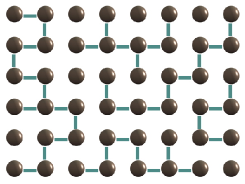
Figure 7: Cubic lattice of a graph state corresponding to the situation where some edges are missing in a cluster state. If the probability $p$ of having an edge is sufficiently high the processes independent, then a renormalized perfect sublattice can be found almost certainly, giving rise to a cluster state of smaller size. If $p>p_{2}=1/2$, where $p_{2}$ is the percolation threshold for edge percolation in 2-D cubic lattices, then a renormalized lattice can be found almost certainly. Interestingly, even if $1/2>p>p_{3}$, $p_{3}=0.249$ denoting the percolation threshold in 3-D, one can almost certainly construct a perfect sublattice, using an overhead that is arbitrarily close to being quadratic.

V One-way computation using encoded systems

In the final section of this work, we will show that one can find resource states for MBQC that differ substantially from the cluster in various entanglement properties. This will be done by encoding each system of a resource into several physical particles. We will not develop any new computational models and make no use of the computational tensor network formalism introduced before. The study of encoded resource states was initiated in Ref. [1] and later pursued more systematically in Ref. [25].

More concretely, the following statements will be proved:

Observation 10 (Resources with weak capabilities for state preparation).

There exists a family of universal resource states such that

• The local entropy of entanglement is arbitrarily small,

• The localizable entanglement is arbitrarily small

and, more strongly,

• The probability of succeeding in distilling a maximally entangled pair out of the resource is arbitrarily small, even if one does not a priori fix the two sites between which the pair will be established.

In particular, the resource cannot be used as a state preparator.

We start from a cluster state vector on $n\times n$ systems, denoted by $|Cl_{n\times n}\rangle$, referred to as logical qubits. As in Ref. [1], we want to “dilute” the cluster state, i.e. encode it into a larger system, by means of invoking the codewords

$$\mbox{$|\tilde{0}\rangle$}:=\mbox{$|0\rangle$}^{\otimes k},\,\,\mbox{$|\tilde{1}\rangle$}:=\mbox{$|W_{k}\rangle$}$$ (377)

for some parameter $k$. The argument relies only on the choice of $|W_{k}\rangle$ as a code word in that we focus on its implications on the localizable entanglement, and for that argument, the state vector $|W_{k}\rangle$ has the desired properties of small local entropy and permutation invariance. However, for encoded one-way computation to be possible, any state vector orthogonal to $\mbox{$|0\rangle$}^{\otimes k}$ may be taken, compare also Ref. [25]. Every qubit of the cluster is subjected to the encoding operation

$$V:=\mbox{$|\tilde{0}\rangle$}\mbox{$\langle 0|$}+\mbox{$|\tilde{1}\rangle$}\mbox{$\langle 1|$}$$ (378)

yielding the diluted cluster $|{\cal D}_{n,k}\rangle$. A set of physical qubits corresponding to one cluster bit will be called a block. As before, by a local measurement scheme we mean a sequence of adaptive local projective measurements, local to the physical systems.

Let us first show again in more detail that such an encoding constitutes no obstacle to universal quantum computation. Each of the code words is orthogonal, and for computation to be possible, we need to do local dichotomic measurements in the logical space. By Ref. [44], any two pure orthogonal multi-partite states on $k$ qubits can be deterministically distinguished using LOCC. By making use of the construction of Ref. [44], this can be done by an appropriate ordered sequence of adapted projective measurements $\pi_{1}\otimes\dots\otimes\pi_{k}$ on the sites of each codeword, giving rise to an arbitrary projective dichotomic measurement with Kraus operators

$$A_{1}:=|\psi\rangle\langle\psi|,\,\,A_{2}:=|\psi^{\bot}\rangle\langle\psi^{\bot}|=\mathbbm{1}-|\psi\rangle\langle\psi|$$ (379)

in the logical space, $|\psi\rangle=\alpha|0\rangle+\beta|1\rangle$ and $|\psi^{\bot}\rangle=-\beta^{\ast}|0\rangle+\alpha^{\ast}|1\rangle$. Hence, one can translate any single-site measurement on a cluster state into an LOCC protocol for the encoded cluster. This shows that $|\Psi\rangle$ is universal for deterministic MBC. This is the argument of Ref. [1] (see also Ref. [25] for a more detailed and extensive discussion on one-way computing based on encoded systems).

In the following we are going to show in more detail that despite this property, we are heavily restricted to use this resource to prepare states with a significant amount of entanglement between two constituents. In fact, we can not even distill a perfect maximally entangled qubit pair beyond any given probability of success. This means that these states are universal resources, but on the level of physical systems utterly useless for state preparation. The given resource is, needless to say, not meant as a particularly feasible resource. Instead, we aim at highlighting to what extent as such the entanglement properties can be relaxed, giving a guideline to more general settings.

Note first that the localizable entanglement $E_{L}$ in these resources can easily be shown to be arbitrarily small: The entropy for a measurement in the computational basis reads $H_{b}(3/(4k+2))$, where $H_{b}:[0,1]\rightarrow[0,1]$ is the standard binary entropy function. Using the concavity of the entropy function, we find

$$E_{L}(\mbox{$|{\cal D}_{n,k}\rangle$}\mbox{$\langle{\cal D}_{n,k}|$})\leq H_{b}(3/(4k+2)),$$ (380)

such that $\lim_{k\rightarrow\infty}E_{L}(\mbox{$|{\cal D}_{n,k}\rangle$}\mbox{$\langle{\cal D}_{n,k}|$})=0$. This means that for two fixed sites, the rate at which one can distill maximally entangled pairs by performing measurements on the remaining systems is arbitrarily small.

This can be seen as follows. We will aim at preparing a maximally entangled state between any two constituents of two different blocks. It is easy to see that within the same block, the probability of success can be made arbitrarily small. We hence look at a LOCC distillation scheme, a measurement-based scheme, taking the input $\rho$ and producing outputs

$$\rho\mapsto K_{j}\rho K_{j}^{\dagger}$$ (381)

with probability $p_{j}=\mbox{tr}(K_{j}\rho K_{j}^{\dagger})$, $j=1,\dots,J$. This corresponds to a LOCC procedure, where each of the measurements may depend on all outcomes of the previous local measurements. Let us assume that outcomes labeled $1,\dots,S$ for some $S\leq J$ are successful in distilling a maximally entangled state.

We start by exploiting the permutation symmetry of the code words. Choose a block $i$ of $|{\cal D}_{n,k}\rangle$. Assume there exists a measurement-based scheme with the property that with probability $p$, the scheme will leave at least one system of block $i$ in a state of maximal local entropy. Then there exists a scheme such that with probability $p$, the scheme will leave the first system of block $i$ in a state of maximal local entropy. At some point of time the scheme is going to perform the first measurement on the $i$-th block. Because of permutation invariance, we may assume that it does so on the $k$-th system of the block. The remaining state is still invariant under permutations of the first $k-1$ systems. Hence there is no loss of generality in assuming that the next measurement on the $i$-th block will be performed on the $k-1$-st system. If the local entropy of any of the unmeasured systems is now maximal, then the same will be true for the first one – once again, by permutation invariance.

Also, it is easy to see that the probability $p$ that a measurement-based scheme will leave any system of block $i$ in a locally maximally mixed state is bounded from above by

$$p<2/k.$$ (382)

Let $p_{1}$ be the initial probability of obtaining the outcome $|1\rangle$ for a $Z$ measurement on this qubit, $p_{1}=|\langle 1|{{\cal D}_{n,k}}\rangle|^{2}$. Clearly,

$$p_{1}<1/k.$$ (383)

We consider now a local scheme potentially acting on all qubits except this distinguished one, with branches labeled $j=1,...,J$, aiming at preparing this qubit in a maximally mixed state. Let $p_{s}$ be the probability of the qubit ending up in a locally maximally mixed state. In case of success, so in case of the preparation of a locally maximally entangled state, we have that $p_{1}(s)=1/2$, in case of failure $p_{1}(f)\geq 0$. Combining these inequalities, we get

$$1/k>p_{1}=p_{s}p_{1}(s)+(1-p_{s})p_{1}(f)=p_{s}/2.$$ (384)

We can hence show that there exists a family of universal resource states such that the probability that a local measurement scheme can prepare a maximally entangled qubit pair (up to l.u. equivalence) out of any element of that family is strictly smaller than $\varepsilon>0$.

Let $p_{i}$ be the probability that a site of block $i$ will end up as a part of a maximally entangled pair. This means that when we fix the procedure, and label as before all sequences of measurement outcomes with $j=1,...,J$, one does not perform measurements on all constituents. Let $I$ denote the index set labeling the cases where somewhere on the lattice a maximally entangled pair appears, so the probability $p$ for this to happen is bounded from above by

$$p\leq\sum_{i\in I}p_{i}.$$ (385)

According to the above bound, $p_{i}<2/k$, giving a strict upper bound of $p\leq 2n^{2}/k$ for the overall probability of success. The family

$$\mbox{$|\Psi_{n}\rangle$}:=\mbox{$|{\cal D}_{n,k(n)}\rangle$},$$ (386)

for $k(n):=2\varepsilon^{-1}n^{2}$ is clearly universal, involves only a linear overhead as compared to the original cluster state and satisfies the assumptions advertised above.

VI Conclusions

In this work, we have shown how to construct a plethora of novel models for measurement-based quantum computation. Our methods were taken from many-body theory. The new models for quantum computation follow the paradigm of locally measuring single sites – and hence abandoning any need for unitary control during the computation. Other than that, however, they can be quite different from the one-way model. We have found models where the randomness is compensated in a novel manner, the length of the computation can be random, gates are performed by routing flows of quantum information towards one another, and logical information may be encoded in many correlation systems at the same time. What is more, the resource states can in fact be radically different from the cluster states, in that they may display correlations as typical in ground states, can be weakly entangled. A number of properties of resource states that we found reasonable to assume to be necessary for a state to form a universal resource could be eventually relaxed. So after all, it seems that much less is needed for measurement-based quantum computation than one could reasonably have anticipated. This new degree of flexibility may well pave the way towards tailoring computational model towards many-body states that are particularly feasible to prepare, rather than trying to experimentally realize a specific model.

VII Acknowledgements

This work has benefited from fruitful discussions with a number of people, including K. Audenaert, I. Bloch, H.-J. Briegel, J.I. Cirac, C. Dawson, W. Dür, D. Leung, A. Miyake, M. Van den Nest, F. Verstraete, M.B. Plenio, T. Rudolph, M.M. Wolf, and A. Zeilinger. It has been supported by the EU (QAP, QOVAQIAL), the Elite-Netzwerk Bayern, the EPSRC, the QIP-IRC, Microsoft Research, and the EURYI Award Scheme.

VIII Appendix

VIII.1 Computing correlations functions

What is the value of the two-point correlation function $\langle Z_{i}Z_{i+k}\rangle-\langle Z_{i}\rangle\,\langle Z_{i+k}\rangle$? In this work, we have only introduced the behavior of the correlation system when subject to a local measurement of a rank-one observable. However, in order to evaluate the correlation function, we need “measure the identity” on the intermediate systems or, equivalently, trace them out. Without going into the general theory [26], we just state that tracing out a system will cause the completely positive map

$$\Phi:\rho\mapsto\sum_{i}A[i]\rho A[i]^{\dagger}$$ (387)

to act on the correlation system.

For the cluster state, using the fact that the bases $\{\mbox{$|0\rangle$},\mbox{$|1\rangle$}\}$ and $\{\mbox{$|+\rangle$},\mbox{$|-\rangle$}\}$ are unbiased, we can easily show that $\Phi^{2}$ is the completely depolarizing channel, sending any $\rho$ to $2^{-1}\mathbbm{1}$. This causes any correlation function to vanish for $k>2$. How does the situation look like for the state vector defined by Eq. (370)? We compute:

$$\Phi:\rho\mapsto\sum_{s=0,1}\mbox{tr}(\rho\,G\mbox{$|s\rangle$}\mbox{$\langle s|$}G^{\dagger})\,\mbox{$|0\rangle$}\mbox{$\langle 0|$},$$ (388)

so for $s\in\{0,1\}$:

$$\Phi(\mbox{$|s\rangle$}\mbox{$\langle s|$})=p\mbox{$|s\rangle$}\mbox{$\langle s|$}+(1-p)\mbox{$|\bar{s}\rangle$}\mbox{$\langle\bar{s}|$}$$ (389)

where $\bar{0}:=1,\bar{1}:=0$ and $p:=|\mbox{$\langle 0|$}G\mbox{$|0\rangle$}|^{2}=\sin^{2}(\pi/m)$. In other words: when acting on the computational basis, $\Phi$ implements a simple two-state Markov process, which remains in the same state with probability $p$ and switches its state with probability $(1-p)$. Now, $\langle Z_{i}Z_{i+k}\rangle$ equals $+2$ if an even number of state changes occurred and $-2$ if that number is odd. So for the expectation value we find

$$\langle Z_{i}Z_{i+k}\rangle = 2\sum_{l=0}^{k+1}{k\choose l}p^{k-l}(1-p)^{k}(-1)^{k}$$

$$= 2(2p-1)^{k}=2(2\sin^{2}(\pi/m)-1)^{k}.$$

VIII.2 Hamiltonian of the AKLT-type state

In Section IV.1 we discussed an AKLT-type matrix product state. It was claimed that the state constitutes the unique ground-state of a spin-1 nearest neighbor frustration free gapped Hamiltonian. It must be noted that in this work, we have not introduced the technical tools needed to cope with boundary effects at the end of the chain. There are at least three ways to make the above statement rigorous: a) treat the statement as being valid asymptotically in the limit of large chains, b) work directly with infinite-volume states [26], or c) look at sufficiently large rings with periodic boundary conditions [27]. Once one chooses one of the options outlined above, the proof of this fact proceeds along the same lines as the one of the original AKLT state, as presented in Example 7 of Ref. [26] (see also Ref. [27]). Indeed, using the notions of Refs. [26, 27] one verifies that

$$\Gamma_{2}:{\cal B}(\mathbb{C}^{2})\to\mathbb{C}^{2}\otimes\mathbb{C}^{2},$$ (391)

$$B\mapsto\sum_{i_{1},i_{2}=1}^{3}\mbox{tr}(BA[i_{1}]A[i_{2}])\mbox{$|i_{1},i_{2}\rangle$}$$ (392)

is injective. Further, if ${\cal G}_{2}:=\operatorname{range}\Gamma_{2}$, it is checked by direct computation that $\dim({\cal G}_{2}\otimes\mathbbm{1}\cap\mathbbm{1}\otimes{\cal G}_{2})=\dim{\cal G}_{2}$. All claims follow as detailed in Refs. [26, 27].

In particular, let $h$ be a positive operator supported on the vector space spanned by:

$$\{|1,1\rangle,|2,2\rangle,-(1/4)|0,0\rangle+|1,2\rangle+|2,1\rangle,$$ (393)

$$-(1/\sqrt{8})|0,0\rangle+|0,2\rangle+|2,0\rangle,$$

$$-(1/\sqrt{8})|0,0\rangle+|0,1\rangle+|1,0\rangle\}.$$

Set $H:=\sum_{i}\tau_{i}(h)$, where $\tau_{i}$ translates its argument $i$ sites along the chain. Then $H$ is a non-degenerate, gapped, frustration free, nearest neighbor Hamiltonian (called parent Hamiltonian in Ref. [27]), whose energy is minimized by the state at hand.

References

• [1] D. Gross and J. Eisert, Phys. Rev. Lett. 98, 220503 (2007).
• [2] R. Raussendorf and H.-J. Briegel, Phys. Rev. Lett. 86, 5188 (2001).
• [3] R. Raussendorf and H.-J. Briegel, Quant. Inf. Comp. 6, 433 (2002).
• [4] H.-J. Briegel and R. Raussendorf, Phys. Rev. Lett. 86, 910 (2001).
• [5] M. Hein, W. Dür, J. Eisert, R. Raussendorf, M. Van den Nest, and H.-J. Briegel, quant-ph/0602096.
• [6] M.A. Nielsen, quant-ph/0504097; D.E. Browne and H.-J. Briegel, quant-ph/0603226.
• [7] M. Hein, J. Eisert, and H.-J. Briegel, Phys. Rev. A 69, 062311 (2004); R. Raussendorf, D.E. Browne, and H.-J. Briegel, ibid. 68, 022312 (2003); D. Schlingemann and R.F. Werner, ibid. 65, 012308 (2002).
• [8] O. Mandel, M. Greiner, A. Widera, T. Rom, T.W. Hänsch, and I. Bloch, Nature 425, 937 (2003).
• [9] M.J. Hartmann, F.G.S.L. Brandao, M.B. Plenio, Nature Physics 2, 855 (2006); A.D. Greentree, C. Tahan, J.H. Cole, and L.C. L. Hollenberg, ibid. 2, 856 (2006).
• [10] C. Cabrillo, J.I. Cirac, P. Garcia-Ferndandez, and P. Zoller, Phys. Rev. A 59, 1025 (1999); D.E. Browne, M.B. Plenio, and S.F. Huelga, Phys. Rev. Lett. 91, 067901 (2003).
• [11] P. Walther, K.J. Resch, T. Rudolph, E. Schenck, H. Weinfurter, V. Vedral, M. Aspelmeyer, and A. Zeilinger, Nature 434, 169 (2005).
• [12] D.E. Browne and T. Rudolph, Phys. Rev. Lett. 95, 010501 (2005).
• [13] D. Gross, K. Kieling, and J. Eisert, Phys. Rev. A 74, 042343 (2006); K. Kieling, D. Gross, and J. Eisert; J. Opt. Soc. Am. B 24(2), 184 (2007).
• [14] H. Haeffner et al., Nature 438, 643(2005).
• [15] G. Vidal, Phys. Rev. Lett. 91, 147902 (2003); R. Jozsa, quant-ph/0603163; I. Markov and Y. Shi, quant-ph/0511069; Y.-Y. Shi, L.-M. Duan, and G. Vidal, Phys. Rev. A 74, 022320 (2006).
• [16] M. Van den Nest, W. Dür, G. Vidal, and H.J. Briegel, Phys. Rev. A 75, 012337 (2007).
• [17] D. Gottesman and I.L. Chuang, Nature 402, 390 (1999); M.A. Nielsen, Phys. Lett. A. 308, 96 (2003); D.W. Leung, quant-ph/0111122.
• [18] P. Aliferis and D.W. Leung, Phys. Rev. A 70, 062314 (2004); A.M. Childs, D.W. Leung, and M.A. Nielsen, quant-ph/0404132 (2004); P. Jorrand and S. Perdrix, quant-ph/0404125 (2004).
• [19] R. Jozsa, quant-ph/0508124.
• [20] F. Verstraete and J.I. Cirac, Phys. Rev. A 70, 060302(R) (2004).
• [21] I. Affleck, T. Kennedy, E.H. Lieb, and H. Tasaki, ibid. 59, 799 (1987).
• [22] V. Danos, E. Kashefi, and P. Panangaden, quant-ph/0704.1263 (2007).
• [23] M.S. Tame, M. Paternostro, M.S. Kim, and V. Vedral, Phys. Rev. A 73, 022309 (2006).
• [24] M. Van den Nest, A. Miyake, W. Dür, and H.J. Briegel, Phys. Rev. Lett. 97, 150504 (2006).
• [25] M. van den Nest, W. Dür, A. Miyake, and H.J. Briegel, quant-ph/0702116.
• [26] M. Fannes, B. Nachtergaele, and R.F. Werner, Commun. Math. Phys. 144, 443 (1992); Y.S. Östlund and S. Rommer, Phys. Rev. Lett. 75, 3537 (1995); U. Schollwöck, Rev. Mod. Phys. 77, 259 (2005); D. Perez-Garcia, F. Verstraete, M.M. Wolf, and J.I. Cirac, quant-ph/0608197; J. Eisert, Phys. Rev. Lett. 97, 260501 (2006).
• [27] D. Perez-Garcia, F. Verstraete, M.M. Wolf, and J.I. Cirac, Quant. Inf. Comp. 7, 401 (2007).
• [28] F. Verstraete and J.I. Cirac, cond-mat/0407066; S. Richter (PhD thesis, Osnabrück, 1994), supervised by R.F. Werner; F. Verstraete, M.M. Wolf, D. Perez-Garcia, J.I. Cirac, Phys. Rev. Lett. 96, 220601 (2006).
• [29] M. Popp, F. Verstraete, M.A. Martin-Delgado, and J.I. Cirac, Phys. Rev. A 71, 042306 (2005).
• [30] B. Schumacher and R.F. Werner, quant-ph/0405174.
• [31] D.L. Zhou, B. Zeng, Z. Xu, and C.P. Sun, Phys. Rev. A 68, 062303 (2003).
• [32] M.A. Nielsen and I.L. Chuang, Quantum computation and quantum information (Cambridge University Press, Cambridge, 2000); J. Eisert and M.M. Wolf, Quantum computing, in Handbook of nature-inspired and innovative computing (Springer, New York, 2006).
• [33] D. Aharonov, W. van Dam, J. Kempe, Z. Landau, S. Lloyd, and O. Regev, quant-ph/0405098.
• [34] S. Bravyi and R. Raussendorf, quant-ph/0610162.
• [35] F. Verstraete, M.A. Martín-Delgado, and J.I. Cirac, Phys. Rev. Lett. 92, 087201 (2004).
• [36] P. Cvitanovic, Phys. Rev. D 14, 1536 (1976); R.B. Griffiths, S. Wu, L. Yu, and S.C. Cohen, Phys. Rev.  A 73, 052309 (2006).
• [37] W. Dür, L. Hartmann, M. Hein, M. Lewenstein, and H.J. Briegel, Phys. Rev. Lett. 94, 097203 (2005); S. Anders, M.B. Plenio, W. Dür, F. Verstraete, and H.-J. Briegel, ibid. 97, 107206 (2006).
• [38] A.Y. Kitaev, Ann. Phys. 303, 2 (2003).
• [39] F. Verstraete, M.M. Wolf, D. Perez-Garcia, and J.I. Cirac, Phys. Rev. Lett. 96, 220601 (2006).
• [40] J. Eisert, K. Jacobs, P. Papadopoulos, and M.B. Plenio, Phys. Rev. A 62, 052317 (2000); D. Collins, N. Linden, and S. Popescu, ibid. 64, 032302 (2001); D. Gottesman, The Heisenberg Representation of Quantum Computers, in S.P. Corney et. al. Eds., Proc. XXII Int. Coll. Group Theor. Meth. Phys. (International Press, Cambridge, 1999); J.I. Cirac, W. Dür, B. Kraus, and M. Lewenstein, Phys. Rev. Lett. 86, 544 (2001).
• [41] F. Verstraete, private communication.
• [42] K. Kieling, T. Rudolph, and J. Eisert, quant-ph/0611140.
• [43] G. Grimmett, Percolation (Springer, Berlin, 1999).
• [44] J. Walgate, A.J. Short, L. Hardy, and V. Vedral, Phys. Rev. Lett. 85, 4972 (2000).
• [45] J. Eisert, Phys. Rev. Lett. 95, 040502 (2005).