Simulating the formation and evolution of galaxies:
Multi-phase description of the interstellar medium, star formation, and energy feedback

Abstract

Context. Modelling the gaseous component of the interstellar medium (ISM) by Smoothed Particles Hydrodynamics in N-Body simulations (NB-TSPH) is still very crude when compared to the complex real situation. In the real ISM, many different and almost physically decoupled components (phases) coexist for long periods of time, and since they spread over wide ranges of density and temperature, they cannot be correctly represented by a unique continuous fluid. This would certainly influence star formation which is thought to take place in clumps of cold, dense, molecular clouds, embedded in a warmer, neutral medium, that are almost freely moving throughout the tenuous hot ISM. Therefore, assuming that star formation is simply related to the gas content without specifying the component in which this is both observed and expected to occur, may not be physically sounded.

Aims. In this paper we seek to improve upon this aspect by considering a multi-phase representation of the ISM in NB-TSPH simulations of galaxy formation and evolution with particular attention to the case of early-type galaxies.

Methods. Cold gas clouds are described by the so-called sticky particles algorithm. They can freely move throughout the hot ISM medium; stars form within these clouds and the mass exchange among the three baryonic phases (hot gas, cold clouds, stars) is governed by radiative and Compton cooling and energy feedback by supernova (SN) explosions, stellar winds, and UV radiation. We also consider thermal conduction, cloud-cloud collisions, and chemical enrichment.

Results. Our model agrees with and improves upon previous studies on the same subject. The results for the star formation rate are very promising and agree with recent observational data on early-type galaxies.

Conclusions. These models lend further support to the revised monolithic scheme of galaxy formation, which has recently been also strengthened by high redshift data leading to the so-called downsizing and top-down scenarios.

1 Introduction

Since almost two decades, N-Body (NB) simulations are the best tool we have to study complex systems such as galaxies and clusters. A number of different recipes have been proposed to model the gaseous component of such systems. The best known is probably the Smoothed Particle Hydrodynamics (SPH) (Lucy 1977; Benz 1990). In brief, it describes the gaseous fluid with a finite number of particles, which are followed in their Lagrangian evolution, and evaluates the values of the physical quantities in each point of the real space by smoothing each particle through a kernel function, peaked in its position. Together with the equations of hydrodynamics it allows us to study mechanical heating and shocks; coupled to gravity described by the well known Tree code (T) by Barnes & Hut (1986), the NB-TSPH method has proved to be very efficient.

Nevertheless, it suffers some limitations. In particular, it seems not to be accurate enough to follow in detail the extreme complexity of the structure and physical processes occurring in a galaxy, which include radiative cooling, star formation, feedback from Supernovae, and chemical evolution (Katz 1992; Mihos & Hernquist 1994; Chiosi & Carraro 2002; Merlin & Chiosi 2006). These processes, apart from requiring sufficient computational power in order to achieve the necessary resolution, also need some kind of different, ad hoc descriptions for the various components. The subject is still at infancy, which in part explains the many uncertainties currently affecting the theoretical models. Star formation is usually expressed by the empiric law of Schmidt (1959), in which the rate is proportional to the gas density, often coupled with some conditions reminiscent of the Jeans stability (see e.g. Gerritsen & Icke 1997; Carraro et al. 1998; Buonomo et al. 2000). If the local gas density obeys the above conditions, gas particles are supposed to be turned into star particles. In the so called sticky-particles algorithm (Levinson & Roberts 1981; Noguchi & Ishibashi 1986) star formation is considered to be enhanced by cloud-cloud collisions.

Different recipes have been tested to introduce the complicated physics of star formation into numerical codes. The most physically grounded, although expensive in computational load, simply consists in creating new star particles of different mass according to a chosen initial mass function (IMF). Obviously this causes a huge growth of the total number of particles, which is well beyond present-day technical capability. The situation is more viable if, assumed a certain mass resolution (initial total baryonic mass in form of gas divided by the number of mass particles used in the simulation), a single star particle is conceived as an assembly of real stars whose mass distribution follows a given IMF. In this context, the total number of baryonic particles does not diverge. Therefore a single gas particle can be turned into a star particle with no serious consequences for the NB-TSPH ecology. What happens inside a star particle is relevant only for the energy and chemical yields but not for the NB-TSPH description as such. This scheme has been followed in a number of studies. For instance, Jungwiert et al. (2001) considers the gradual formation of stars inside gas particles, which eventually become star particles when the hidden star mass exceeds a certain threshold value. Along this line of thought is the probabilistic description of star formation by Buonomo et al. (2000); Lia et al. (2002), in which gas particles are turned into star particles according to the Schmidt law however interpreted in statistical sense, so that at any time there is a certain probability that a gas particle becomes a star particle. This way of looking at the star formation process is particularly advantageous in numerical simulations as it keeps constant the total number of particles, thus saving lots of computational time.

Owing to the current mass resolution of numerical simulations, the star particles actually have the mass size of a star cluster, in which the real stars are born in a short burst of intense local activity with homogeneous age and chemical composition. Therefore each star particle can be approximated to a single stellar population (SSP), in which the stars distribute in mass according to some IMF.

The influence of the IMF describing the stellar content of each star particle becomes soon evident when the energy and chemical feedback by supernova (SN) explosions and/or stellar winds to the surrounding medium are taken into account. Several unsettled questions come soon into play. Among others, it is still not clear whether the SN energy feedback should be only treated as ”thermal” or if some kinetic effects have to be considered (see e.g. Marri & White 2003). How to share chemical elements ejected by a star particle with the surrounding medium is another point of uncertainty. Also in this case the statistical description by Lia et al. (2002) turns out to be particularly convenient.

In current NB-TSPH models, the gas component is considered as an unique fluid regardless of the observational fact that in the gas content of real galaxies several different phases are present: hot and cold, tenuous and dense, ionised, neutral and molecular gas. Furthermore, in the same models star formation and its efficiency are related to the total gas content with no attention to the observational fact that stars are formed only in dense molecular clouds. In this paper, we present a multi-phase description of the ISM (hot gas and cold clouds with molecular cores inside) in which star formation can occur only in the cold component thus bringing the simulations closer to reality. The new prescription for the ISM is implemented in GalDyn, the Padua NB-TSPH code originally developed by Carraro et al. (1998) and later improved by Lia et al. (2002) and Merlin & Chiosi (2006).

The layout of the paper is as follows. In Sect. 2 we present in some details the physical problem and briefly summarize our prescription for the ISM and how it is implemented in the numerical code. In Sect. 3 we test the new method simulating the formation of an early-type galaxy and present the results. In Sect. 4 we discuss the results, compare them to some recent observational data on galaxy formation and evolution, and draw some general conclusions.

2 Multi-phase ISM

2.1 The physical context

Since the early sixties, the ISM in the Milky Way is known not to be uniform on small scales, but to contain strong local density enhancements, so that very dense and cold regions, in form of atomic and molecular ”clouds”, appear to be embedded in a diffuse hot, ionised medium (Field et al. 1969). Some years later, with the increasing understanding of the importance of SN explosions, another component was introduced, i.e. the hot and very tenuous coronal gas expelled by exploding stars (McKee & Ostriker 1977).

Therefore, it is nowadays widely accepted that the ISM of the Milky Way is made of several components with different temperatures and densities. At least four, almost decoupled, gaseous phases are present: (i) the hot, highly or fully ionised, tenuous medium, with temperatures of some tens of thousands of Kelvin degrees and number densities of about 0.1 cm^-3; (ii) the cold, dense, clumpy molecular medium, with temperatures of only a few Kelvin degrees and number densities from thousands up to millions of atoms per cm³; (iii) a cloud-embedding, warm, neutral phase, with temperatures from a few thousands down to a few hundreds Kelvin degrees, and number density of a few atoms per cm³; (iv) and an extremely hot and rarefied coronal gas expelled by the SN explosions, with temperatures of millions of Kelvin degrees and very low number densities (some 0.01 atoms per cm³). Of course, this scheme is still a simple one, because the ISM contains other local features (HII regions, for instance, which are regions of ionised and hot but very dense material).

In the Milky Way, these different phases fill the interstellar space in a way that is inversely proportional to their density. Most of the space is filled by the coronal and hot gas, whereas only a minor fraction of it is filled by the cold clouds. The cold clouds, on the other hand, contain the largest fractional mass of the ISM. Owing to such a strong density contrast, the cold clouds are not strongly affected by drag interactions with the tenuous phase (see Levinson & Roberts 1981, , and below).

Given this situation, it seems clear that the SPH algorithm, which is fully adequate to describe a single-phase fluid even in situations of shock, cannot be considered the best tool to study such a complex mixture of different phases in mechanical and thermodynamical equilibrium. A well known problem of the SPH method, for instance, is the so called overcooling. Considering the whole mass of gas as a single fluid, a particle can have neighbouring particles with much higher densities. These should actually be considered as part of another decoupled phase. In the SPH formalism they actually end up to dominate the local density of the particle under consideration, thus leading to overestimate the density and consequently to a stronger, un-physical radiative cooling (see Marri & White 2003).

Furthermore, the correct equation of state relating pressure, density, temperature, and chemical composition of the gas should properly include the molecular component. In most numerical NB-TSPH codes including our own, the equation of state is that for an ideal mono-atomic gas, which obviously does not adequately describe the molecular component. Finally, self-gravitating molecular clouds are known to obey particular empirical laws (e.g. Larson 1981). Likely, they should be taken into account in the grand-design of star formation.

Over the years, many attempts have been made to solve this problem and to find a physically sounded recipe for star formation in molecular clouds. Levinson & Roberts (1981) developed the so called sticky particles algorithm, in which the ISM is modelled only by means of clouds freely moving across the surrounding void space. More recently, Marri & White (2003) suggested a simple modification of the neighbour searching algorithm in SPH: particles of very different density and temperature are discarded in the neighbour sampling. Other strategies have been recently proposed by Semelin & Combes (2002), Harfst et al. (2006) and Booth et al. (2007), trying to simulate the evolution of disk galaxies.

A description of the ISM as detailed as possible is required also to study galaxy formation in cosmological context. Even if there are no evidences that the primordial ISM was similar to the present-day ISM in the Milky Way, nor the contrary, it is likely that the ISM always had an important role. In particular, the duration and intensity of the star formation activity should be strongly dependent on how different components of matter interact each other. Along this line of thought are the attempts made by Springel & Hernquist (2003) to reproduce the complexity of the ISM in cosmological context.

2.2 The multi-phase prescription

Starting from these considerations and the above mentioned studies, we tried to elaborate a recipe for the various components of the ISM and their relationships. In brief, hot gas is slowly turned into cold clouds and star formation occurs in these latter. Viceversa the energy deposit by dying stars heats up the cold gas. The key points of our recipe are the listed below.

(1) We assume that the SPH method can reasonably describe the hot phase of the ISM, considering as ”hot” the gas particles which are hotter and less dense than suitable temperature and density thresholds (i.e. both the hot ionised gas and the coronal gas).

(2) The cold phase (molecular clouds), in which star formation occurs, is described by a different method, based on the fact that individual particles can roughly represent single clumps of cold material. A giant molecular cloud can reach a mass of some $10^{6}\,M_{\odot}$. Considering also the embedding neutral or slightly ionised warm material, the total mass of a cold particle can be higher than this value. As discussed below, the mass resolution of our fiducial model is close to $6\times 10^{6}\,M_{\odot}$ thus making our description quite realistic.

(3) Following Levinson & Roberts (1981), we assume that the cold clumps can move almost freely throughout the hot phase. Pressure drag and friction are certainly present, but we consider them negligible for our purposes.

(4) As suggested by Semelin & Combes (2002), a hot gas particle does not instantaneously turn into a cold cloud particle when its temperature falls below the threshold value because letting this to occur would originate too sharp a transition. Therefore, we prefer to use a smooth procedure named gathering method. Each gas particle is thought to be made of gas at different temperatures distributed according to a gaussian law, truncated at $2\sigma$ from the central peak determined by the SPH value. To some extent, this mirrors the situation of the SPH technique, in which each particle has properties that result from averaging those of nearby particles, so that only groups of particles can be considered as representative of the distribution of matter in a given region. The $\sigma_{cold}$ of this quasi-gaussian distribution is a free parameter. Each particle is then assigned a certain fraction of cold gas, i.e. the amount of gas in the quasi-gaussian distribution whose temperature falls below the threshold value $T_{cold}$. At each time step, a particle tries to ”acquire” some cold gas from its SPH neighbours until a single cold particle of mass equal to that of the mother particle is formed. When this is achieved, a new ”cold” particle is created from the ”hot” one. The cold particle is separated from the surrounding hot medium, provided it belongs to a convergent flow (i.e. its velocity divergence is negative), and its cooling time is shorter than its dynamical time, whose evaluation takes Dark Matter around into account (Buonomo et al. 2000). The temperature $T_{HI}$ of the new cold particle is determined by the condition that during the creation process the total thermal energy of the group of particles remains constant, together with the requirement that neighbours have no longer cold gas (their temperature distributions accordingly vary). If the temperature of a gaseous hot particle is limited by the Jeans threshold (see Sect. 3.1, point 3), its $\sigma_{cold}$ is changed so that it can provide some small fraction of cold gas anyway. The limitation imposed by the Jeans threshold is indeed a numerical artifact due to resolution limits, and there are no real physical reasons to exclude the presence of a small fraction of cold gas within the total gaseous mass of the particle. The $\sigma_{cold}$ is adjusted in such a way that the lower limit of the truncated gaussian distribution corresponds to zero temperature.

Finally, we assign the new cold particle the initial density obtained by interpolating with a cubic polynomial fit the relation between temperature and number density given by Scheffler & Elsaesser (1987) for cold clouds in pressure equilibrium with the surrounding medium:

$$log[n_{HI}]=-0.943x^{3}+8.3x^{2}-24.66x+23.5,$$ (1)

where $x=log[T_{HI}]$. The relation in shown in Fig. 1.

Figure 1: Number density versus temperature of atomic Hydrogen in pressure equilibrium.

(5) In addition to gravity, the only interactions that cold particles can feel are the mutual inelastic collisions (Levinson & Roberts 1981).

Collisions between clouds are known to trigger star formation (Loren 1976; Hasegawa et al. 1994), due to the creation of a hot shock front which rapidly cools down causing fragmentation in cold, extremely dense cores of molecular gas. Numerical simulations of the impact between two clouds (Marinho & Lépine 2000; Marinho et al. 2001) showed how the results of such impacts depend on many parameters, often acting well below our resolution scale. Anyway, based on those simulations as well as on the cited observational evidences, we can envision the following scenario. First of all, two clouds are considered to be colliding if their mutual distance is shorter then the sum of the radii of each particle. A rigourous description of cloud-cloud collisions would require the use of the impact parameter instead of the distance. However, in the framework of the statistical approach used for star formation and gas restitution (see below) using the distance is adequate to our purposes. The radius of a particle is derived from its mass to total density ratio and the assumption of spherical symmetry. The total density and mass include both the neutral and the molecular components. Second, the densities of the two colliding particles must be comparable. If this is not the case, the denser cloud will likely cross the less dense one without feeling sizeable effects. Therefore, we assume that to have a collision the mean densities of the two colliding clouds should not differ by more than a factor of ten. Finally, depending on the mutual distance two kinds of collisions are possible:

• The head-on collision, which happens if the distance between the clouds becomes shorter then their mean radius. In this case, the kinetic energies of the colliding particles are decreased to $20\%$ of their original values, the directions of the colliding components of the velocity vectors are reversed, and the molecular density of both particles is increased by a factor of 100.

• The off-centre collision, which happens if the distance between the clouds gets shorter than the sum of the two radii but larger than their mean radius. then their mean radius In this case, the molecular densities are increased by a factor of 10 and the kinetic energies are decreased to $80\%$ of their initial value.

• No interaction is supposed to occur in all other circumstances.

Clouds are allowed to experience collisions until they reach the molecular density of $10^{-18}\mbox{g/cm}^{3}$. All assumptions are consistent with the results of the Marinho & Lépine (2000) simulations.

(6) The internal evolution of the clumps goes as follows. Each ”cold particle” represents a self-gravitating portion of the ISM in which two gas phases at different densities and temperatures coexist, i.e. the molecular core of the cloud and the surrounding warmer material. We cannot determine the temperature and density of the two components, because physical processes at these scales are below the resolution power of our simulations. It is known that in cold collapsing clouds the ”fragmentation” process can break them into pieces when the density exceed the value set by the Jeans stability condition. As already anticipated, we cannot use the perfect gas equation of state for the molecular part of the clouds, because different laws are expect to hold (i.e. Larson 1981) and complicated processes such as turbulence and magnetic interactions may play very important roles in the molecular core. To partly get rid of this difficulty, starting from the study of Springel & Hernquist (2003) in cosmological context, we describe the cold cloud using mean values that refer to the ”molecular part” and the ”neutral” embedding warmer phase, and assume that in the cold particle, radiative cooling causes the increase of $H_{2}$ phase at the expenses of the $HI$ phase (the process is occurring at constant temperature for the two components) according to:

$$\frac{\delta\rho_{H_{2}}}{\delta t}=-\frac{\delta\rho_{HI}}{\delta t}=\frac{\Lambda_{HI}(\rho_{HI},u_{HI})}{u_{HI}-u_{H_{2}}}\rho_{HI}.$$ (2)

In practice, when a gas particle detaches itself from the surrounding hot ambient medium and becomes a ”cloud”, it is thought to be made of molecular and neutral gas in some proportions (in our simulations, we assume that no $H_{2}$ is present when the cloud is formed and it increases afterwards). The radiative losses ”cool” the neutral part and the ”cooled” material is subtracted from it and accreted onto the molecular part, thus changing the densities of the two phases (at constant occupational volume).

(7) Only cold particles are allowed to form stars. The transition from cold gas particles to star particles is based, as explained in Lia et al. (2002), on a probabilistic interpretation of the Schmidt (1959) law. In practice, we consider that on a time scale of about 3 Myr (the lifetime of a typical high mass star) a fraction of the molecular gas, proportional to its density, is turned into stars according to

$$\frac{d\rho_{*}}{dt}=c_{*}\frac{d\rho_{H_{2}}}{t_{dyn}}.$$ (3)

Instead of creating more and more new particles of different mass, which would make the computational cost too high, we prefer to interpret this formula as the probability that a cloud particle is completely turned into a star particle. The probability is

$$P(SF)=\left[\frac{\rho_{H_{2}}}{\left(\rho_{H_{2}}+\rho_{HI}\right)}\right]\left[1-exp\left(\frac{-c_{*}\Delta t}{t_{dyn}}\right)\right]\,,$$ (4)

where the first term takes into account that we consider only the molecular density when turning the whole particle into stars. Buonomo et al. (2000) showed that, provided the total number of particles is sufficiently high (say more than $\simeq 2000$), the right global behaviour is achieved (the statistical description equals the straight one). Following Lada & Lada (2003), we adopt $c_{*}=0.05$. As already mentioned, close encounters between clouds enhance star formation, due to the growth of molecular densities after a collision.

(8) Along with radiative cooling and energy dissipation by inelastic collisions, the thermal evolution of clouds is governed by the energy input by SN explosions. The SN energy feedback is perhaps the most difficult issue to address, because of its complex and poorly known physics. Furthermore, all physical processes concerning SN explosions and evolution of the SN remnants (SNR) are well below both our time and space resolution scales (namely, $\sim$ 1 Myr and $\sim$ 1 kpc), so that we are forced to represent them through ”global” changes on large ISM regions. Here we adopt a simple description and try to minimize the number of free parameters.

feedback energy from SN explosions is distributed among particles as follows. The ”death” of star particles and associated SN explosions are described with the statistical method proposed by Lia et al. (2002), see also Merlin & Chiosi (2006). In brief, a star particle (a SSP of a certain age) is sorted out through a Monte-Carlo method and its ”death probability” is measured by the ratio between the amount of mass lost by stellar winds and SN explosions and total SSP mass. The probability goes from zero to one when the ratio goes from ”zero to one” (from zero to a maximum value that ultimately depends for a given IMF on the mass interval within the SSP in which SN explosions are supposed to occur). In this way, we avoid instantaneous recycling and, at increasing number of star particles, we get closer and closer to a realistic description. When a star particle dies, its mass is completely turned back to the hot phase, and the energy feedback due to SN explosions within the SSP is spread over the particle itself and its neighbours, in the following way. First of all we compute the total gaseous mass $m_{tot}$ inside a sphere of radius equal to the smoothing length of the newly born gas particle. $m_{tot}$ is thus given by the mass of the particle itself plus the mass of all cold clouds inside the sphere of radius equal to the smoothing length. The corresponding release of specific energy $u$ [$erg/g$] is

$$u=\frac{N_{SN}E_{th}}{m_{tot}},$$ (5)

where $N_{SN}$ is the number of SN explosions within the dying particle, calculated according to the Greggio & Renzini (1983) rates, and $E_{th}$ is the thermal energy produced by each explosion (see below). Each cloud is then given an amount of thermal energy corresponding to its mass, decreased accordingly to the smoothing kernel of the newly formed gas particle, and the exceeding energy is given to the new gas particle and added to its original thermal energy. Furthermore, thermal energy is spread among the hot neighbouring particles according to the normal SPH algorithm. Following Thornton et al. (1998), we assume that the amount of thermal energy spread over the ISM by each SN explosion (which yields a total energy of $10^{51}$ ergs per event) depends on the ambient gas conditions. Thus, we compute the mean values of density and metallicity $n_{0}$ and $Z/Z_{\odot}$ of the neighbouring particles, weighing each contribution on the smoothing kernel, and use the following relation to obtain the total amount of thermal energy to be spread into the surrounding medium (see Thornton et al. 1998, for details):

$$E_{th}=1.83\times 10^{49}n_{0}^{-0.23}(Z/Z_{\odot})^{-0.24}$$

$$+1.23\times 10^{49}n_{0}^{-0.24}(Z/Z_{\odot})^{-0.08}ergs,$$ (6)

if $log[Z/Z_{\odot}]>-2$, and

$$E_{th}=5.53\times 10^{49}n_{0}^{-0.23}$$

$$+1.78\times 10^{49}n_{0}^{-0.24}ergs$$ (7)

otherwise. Finally, each cloud is given an amount of radial kinetic energy, still weighed on the kernel and computed in the same way as for the thermal energy, using the empirical relation $E_{kin}=1.69\times 10^{50}$ ergs of Thornton et al. (1998).

With this mechanism, clouds are allowed to ”evaporate” back to the hot phase as soon as the temperature of their neutral part gets higher than a threshold value, that is naturally taken equal to the cloud formation temperature. In addition to this, we try to mimic the first phase of adiabatic expansion of the SNR and passage of the compressional front (see McKee & Ostriker 1977, for details) by momentarily inhibiting radiative cooling in clouds which experience SN heating. By doing this we ensure that sudden cooling of the particles cannot take place simply because soon after the explosion they happen to be immersed in a denser environment.

(9) Finally, the chemical evolution of the ISM is followed as in Lia et al. (2002). It is worth noting, however, that cold particles are supposed not to experience chemical enrichment, which is limited to the hot medium. Only when a cloud has been evaporated by SN energy feedback it can enrich its gas with metals.

Fig. 2 shows a schematic summary of the different interactions among the baryonic components of a model galaxy with the new scheme.

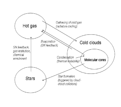
Figure 2: The different interactions among the three baryonic components of a galaxy with the multi-phase description of the ISM.

3 Testing the new recipe

3.1 GalDyn, The Padova NB-TSPH code

GalDyn is an evolutionary code for galactic systems, developed in Padova over the years. It is a fully lagrangian NB-TSPH code, based on the well known Tree-code by Barnes & Hut (1986) and SPH algorithm by Lucy (1977). For a detailed description of the basic version of the code see Carraro et al. (1998); Buonomo et al. (2000); Lia et al. (2002); Merlin & Chiosi (2006). For the purposes of this study, the code has been improved in several ways with respect to the previous versions.

(1) First of all, an adaptive multiple time-step integration scheme has been adopted. For each particle an individual time-step taken as the minimum between the acceleration time-scale, the velocity time-scale, and, for gas particles, the Courant time-step (see Merlin & Chiosi 2006, for details) is calculated using its current physical values. Within each time-step for the whole system, only those particles with a sufficiently small individual time step are considered to be ”active” and are moved on, using a Drift-Kick-Drift Leapfrog integrator. This is similar to the implementation used by Springel et al. (2001) in Gadget 1. However, it is worth noting that the Drift-Kick-Drift algorithm may suffer non negligible problems for what concerns the conservation of the motion integrals (see Springel 2005). Note that particles are not allowed to have a time-step lower than a minimum value (fixed equal to $10^{-5}$ of the Hubble time), and whenever required their smoothing length is changed to establish the right value.

(2) The adopted smoothing kernel for SPH particles, originally developed by Monaghan & Lattanzio (1985), has been revised following Thacker et al. (2000) and references therein. In order to avoid artificial clumping in high density regions, the first derivative of the kernel function is set constant and equal to $1/(\pi h^{3})$ for small radii.

(3) Radiative cooling is not allowed to be active on a particle when its temperature falls below the threshold value given by

$$T_{min}=C\left[\left(\frac{4m_{p}}{\rho_{g}}\right)^{2/3}-\left(\frac{\pi\epsilon_{g}^{3}}{3}\right)^{2/3}\right]\frac{\mu m_{H}G}{k}\rho_{g},$$ (8)

(see Bonnor 1956) where $m_{p}$ is the mass of a baryonic particle, $k$ is the Boltzmann constant, $\mu$ and $\epsilon$ are the mean molecular weight and the gas softening parameter, $m_{H}$ is the proton mass, and the C is a constant (in cgs units, C=0.89553). Below this temperature the particle would become Jeans unstable (obviously, adiabatic cooling is not limited by this condition). This somehow imposes an unavoidable limit to the mass resolution of the particles because, if the threshold value is too high, cooling and cloud formation cannot be correctly modelled. In Fig. 3 the threshold temperature in Kelvin degrees is plotted versus the logarithm of density (in g/cm³), for several values of the particle masses and softening lengths. The solid lines refers to the values adopted in the present simulations, see Sect. 3.2.

(4) In order to correctly evaluate the impact of the inverse Compton cooling at high redshifts, we roughly estimate the ionization fraction and thus the number density of free electrons as a function of temperature. The number density is

$$n_{e}=n_{HI}\mbox{ if }T\geq 10^{4}\mbox{ K,}$$

$$n_{e}=n_{HI}\times exp(-(10^{4}-T))\mbox{ otherwise,}$$ (9)

where the value of $10^{4}$ K roughly corresponds to the ionization temperature of Hydrogen in astrophysical environments.

(5) We describe the thermal conduction among SPH particles as originally developed by Monaghan & Lattanzio (1991). Thermal conduction is expected to be important in situations of shocks, and in particular after a SN event. McKee & Ostriker (1977) pointed out that thermal conduction could evaporate cold clouds and warm up the ISM inside a SNR (thus also changing the density inside the remnant). Although in our scheme clouds are evaporated ”automatically” due to SN events, we expect thermal conduction to be important in the subsequent phases of evolution, when a large number of hot particles are present in a high density region.

(6) To take into account UV flux and stellar winds from massive stars without too much computational effort, we make use of the results of Buonomo et al. (2000) who found that the contribution to the energy feedback by these two sources of energy is comparable to that of SN. Since stellar winds and UV flux come the same stars that eventually will explode as Type II SN, we crudely lump together the three contributions and simply increase by a factor of 3 the energy injection by SN explosions.

Figure 3: Lower threshold temperature for SPH particles of mass $m_{p}$ and softening length $\epsilon$, as a function of their density. Solid line: $m_{p}$ = $m_{0,p}$ = $6\times 10^{6}$ M_⊙, $\epsilon$ = $\epsilon_{0}$ = 1 kpc. Dotted lines: from top to bottom, $m_{p}$ = $m_{0,p}$ and $\epsilon$ = 0.1, 0.5, 2 times $\epsilon_{0}$. Dashed lines: from top to bottom, $\epsilon$ = $\epsilon_{0}$ and $m_{p}$ = 2, 0.5 and 0.1 times $m_{0,p}$.

3.2 Formation of a galaxy in cosmological context

We have tested the new prescription for star formation implemented in GalDyn by simulating the formation of a galaxy from quasi-cosmological initial conditions.

The cosmological scenario we adopt is consistent with the W-Map3 results (Spergel et al. 2006), namely $h_{0}=0.73$, $\Omega_{m}=0.238$, $k=0$, $\sigma_{8}=0.74$, $n=0.951$, and initial baryon fraction $\sim 17.6\%$.

The initial conditions are obtained using the Grafic2 package by Bertschinger (2001) to generate an initial perturbed cubic grid of 64³=262,144 particles. In this grid we search a region containing an overdensity peak and single out another much smaller cubic volume around it, so that the peak is located near its geometrical centre. This small cubic region is initially made of 6³=216 particles (corresponding to a cubic volume of $\sim 20^{3}$ physical kpc³) and is then re-simulated with a finer resolution, which is imposed to give at the end a number of particles compatible with our computing capability. Finally, in the re-simulated small cubic volume we isolate the sphere whose radius is half of the cube dimension and whose centre coincides with that of the cube (i.e., with the original position of the density peak in the large cubic grid). This final sphere contains $\sim$ 14,000 particles (approximately half of dark matter and half of baryons). The sphere is inserted into the conformal Hubble flow with void boundary conditions. These latter may not be fully adequate to describe the real situation because the isolated volume is in reality immersed in a background exerting some dynamical effects on the matter contained inside the sphere under consideration. To cope with this, we add a small initial solid-body rotation to the sphere, and follow its expansion, detaching from the Hubble expansion, turn-around, and collapse (see e.g. Merlin & Chiosi 2006, for details on the initial conditions). The sphere can be considered as a good approximation of an isolated initial proto-galaxy. Despite the small solid body rotation, the void boundary conditions may cause some problems, which anyway are not crucial for our purposes (see Merlin & Chiosi 2006, for more details).

As already said, the way the cubic volume single out from original grid has been re-simulated is chosen in such a way that the total number of particles in the so-called proto-galaxy is compatible with our limited computing facilities. We are well aware that the rather small total number of particles may constitute a major drawback of the results we are going to present. The main motivation for this choice is that we want to test the new scheme of star formation with an affordable computing cost and time. However, several studies (see e.g. Kawata 1999; Buonomo et al. 2000; Kawata 2001a, b; Kawata & Gibson 2003; Semelin & Combes 2002) have already shown that a total number of particles of the order of $10^{4}$ is enough to achieve a sufficiently accurate global description of the physical processes. Therefore, we are confident that the main body of the physical conclusions we are presenting are not too badly influenced by resolution limits. They have to be viewed as indications of the right trail to follow in the future.

We also consider the action of the re-ionizing background radiation (e.g. the UV field of the PopIII massive stars). To deal with effect in a very simple way, we crudely add a constant heating of $10^{-24}$ ergs/s/atom from redshift z=20 to z=6.

As the simulation starts well before re-ionization and the initial overdensity of the proto-galactic halo is small, Hydrogen can be considered as almost completely neutral at the initial stage. Anyway, the initial temperature of the gas is set equal to the maximum between a ”cosmological” value, obtained as explained in Merlin & Chiosi (2006), and the minimum temperature allowed by the Jeans limit discussed above. Indeed, the cosmological temperature of baryonic matter at $z\sim 60$ would be below 100 K, but the Jeans resolution in the present models imposes a threshold value of $\sim 2000$ K. As the Jeans threshold is well below the value at which ionization is expected to yield sizeable effects, we can safely use this value instead of the real cosmological limit. In any case, at the very initial stage we must consider the gaseous component as made only by ”hot” particles, because as already explained, cold clouds are allowed to form only when belonging to collapsing flows.

Ballesteros-Paredes et al. (2007) estimated the following densities and temperatures for the two main components of a cold cloud: $1<n<100$ cm^-3 and $100<T<5000$ for the atomic gas; $100<n<1000$ cm^-3 (up to $10^{6}$ in cores) and $10<T<100$ K for the molecular gas. Therefore, we adopt $T_{cold}=5000$ K and $\rho_{cold}=10^{-27}$ g/cm³ as threshold values. Such a low value for the density threshold is motivated by the fact that this is the global SPH density of a particle, while in order to create cold clouds we are only interested in the densest part of it. We then choose $\sigma_{cold}=1000$ K. Finally, to describe the properties of of our star particles (energy feedback and chemical enrichment) we adopt the Salpeter (1955) IMF.

Our model proto-galaxy has an initial radius of $19$ kpc, and a total (Dark and Baryonic) mass of $2.5\times 10^{11}M_{\odot}$, with an overdensity of $\simeq 0.09$ at the initial redshift $z=60$. The number of particles for Baryonic and Dark Matter is $\simeq 7000$, the same for each component. For baryons the mass of a particle is $\simeq 6\times 10^{6}M_{\odot}$, and the softening length is 1 kpc; the corresponding values for the Dark Matter component are $\simeq 3\times 10^{7}M_{\odot}$ and 2 kpc, because of the much higher total mass. All the relevant quantities in use are summarized in Table 1.

Table 1: Initial parameters for the model proto-galaxy

Initial redshift	60
Initial mean overdensity	0.09
Initial radius [kpc]	19
Total mass [$M_{\odot}$]	$2.5\times 10^{11}$
Number of baryonic particles	7000
Mass of a baryonic particle [$M_{\odot}$]	$6\times 10^{6}$
Softening length for a baryonic particle [kpc]	1
Number of Dark particles	7000
Mass of a Dark particle [$M_{\odot}$]	$3\times 10^{7}$
Softening length for a Dark particle [kpc]	2

Figure 4: From top to bottom, from left to right: position (physical Mpc) of Dark Matter particles projected on the XY plane at redshift $z=5.9,3.4,1.7,1.0$.

Figure 5: Same as above, but for hot gas particles.

Figure 6: Same as above, but for cold gas particles.

Figure 7: Same as above, but for star particles.

Figure 8: Fractional mass in the three baryonic components versus time. Dashed: hot gas; dotted: cold clouds; solid: stars.

3.3 Formation and evolution of a galaxy: results and comments

First of all, we note that owing to the present procedure to isolate the proto-galaxy from the cosmological context, the void boundary approximation may influence the evolutionary time scales and the detailed results in turn. In particular, it may (slightly) change the relationship between rest-frame evolutionary time and redshift (see Merlin & Chiosi 2006). Despite this cautionary remark, we are rather confident that the basic features and properties of the model should not depend very much from this drawback of the present formulation.

Figure 9: Star formation rate in solar masses per year.

Galaxy formation. In Figs. 4 through 7 we show the spatial evolution of the system, in its four components: Dark Matter, hot gas, cold clouds and stars. All boxes are 100 kpc per side. The number of cold clouds (whose dimensions have been magnified for clarity) is always quite small, as they soon evolve into stars or are evaporated back to the hot phase; this is clearly visible in Fig. 8 showing the fractionary mass of the baryonic components as a function of the cosmic time. This situation, which differs from the one in a disk galaxy like the Milky Way, where most of the gaseous mass is stored in the cold phase, can be explained as follows. First, there is a technical reason: as already noted, at the beginning of the simulation, in order to apply the SPH formalism and get the right values for densities and temperatures, we consider the gaseous component to be made only by hot particles, even if their temperature is below the threshold value for cloud formation. This effect should become less relevant as the galaxy ages. Second, the mass resolution is small, so that statically the number of cold clouds going into stars per time step is also small (and fluctuating). The third reason is more physical: in our model galaxy (simulating what happens in an elliptical) a large fraction of gas is turned into stars so that little gas is left after a few Gyr of star formation activity (see below). Most of the cold gas sinks very early toward the centre of the proto-galaxy, whereby undergoing frequent collisions is turned into stars at a high rate. Dying stars soon provide SN feedback to the surrounding medium, thus inhibiting the formation of a great number of new cold clouds. Conversely, in situations with low star formation rates (such as in evolved disk galaxies) the cold gas is expected to distribute almost uniformly across the disk and likely to co-rotate with the rest of the galaxy; the number of cloud-cloud collisions is of course lower and lots of cold gas survive to star formation. See below for some additional comments on this issue.

The clumps of collapsed matter merge at very early times, and at $z\simeq 3.5$ the main body of the final object is in place, accreting new material from the outskirts. In the context of current terminology in literature, we prefer to classify this situation as ”monolithic” rather than ”hierarchical”. In any case it would be a ”very early hierarchical” assembly of a galaxy. At the end of the simulation ($z\simeq 0$), the galaxy has a nearly spherical shape with axial ratios $b/a=1.02$ and $c/a=1.12$. The total stellar mass is $\simeq 3\times 10^{10}M_{\odot}$ ($75\%$ of the initial baryonic mass), with an half mass radius $R_{1/2}=4.6$ kpc. Almost no gas is left inside the virial radius of the object.

In Fig. 9 the rate of star formation (in solar masses per year) is shown. The first stars begin to form around $z\simeq 12$. The bulk of stars (80% of the total) is in place at $z\simeq 1.6$. The galaxy has already acquired its final features, and from now on it evolves almost passively. The last, minor burst of star formation takes place at $z\simeq 0.7$. These result is in good agreement with the observations for objects with similar total stellar mass (see e.g. Thomas et al. 2005; Clemens et al. 2006; Cimatti et al. 2006). In the nowadays well-established downsizing scenario, smaller objects assemble their stellar content over longer time scales than massive galaxies - at least in high density environments. Among others, Jimenez et al. (2005) studied a large sample of $\simeq 10^{5}$ galaxies from the SDSS, and found a tight relation between the total stellar mass of an object and epoch of its assembly (see e.g. their Fig. 4). A system with $10^{10}<M_{*}/M_{\odot}<10^{11}$ is expected to form most of its stellar content about $\simeq 5-6$ Gyr ago, whilst more massive objects are expected to exhaust their activity much earlier (the situation being more intrigued for low mass objects, which have different histories depending on their initial overdensity). Our results are in very good agreement with this picture, and no particular fine tuning of parameters was required to obtain them. Indeed, all the parameters are conservative and taken from previous studies of both observational and theoretical nature. Perhaps, a more prolonged period of activity could have been expected for our object, given its mass and its rather low initial overdensity, but of course we cannot too strictly compare the results for a single model galaxy with the statistically averaged trends that are found observationally.

In order to achieve some insights on this point, as well as on the improvements due to the new prescription for star formation, we compared the present results with those obtained with the classical SPH treatment of the ISM (see Merlin & Chiosi 2006, for details). The two star formation histories are shown in Fig. 10, where the solid lines are polynomial best fits of the numerical results, sketched in order to give an idea of the trends of the star formation histories in the two models apart from the very fluctuating profiles, which are due partly to numerical artifacts and partly to the statistical method we have adopted to deal with star formation and energy injection by dying stars. The SPH simulation was stopped after 7 Gyr of evolution due to limited computational resources. With the new prescription, the formation of the stellar mass is more gradual and lasts longer; the peak of activity is lowered from $\simeq 17$ to $\simeq 12$ solar masses per year, and shifted from $z\simeq 4.3$ to $z\simeq 2.9$. The total stellar mass assembled in the two models is, however, almost equal. The different behaviour obtained with the two star formation prescriptions can be understood first of all by looking at the different time scales involved in the formation of new stars. In the classical SPH treatment, all gas particles can in principle be turned into stars, and therefore a large reservoir of fuel is ready to be used right from the beginning, giving rise to a strong and sudden burst of activity. In contrast, with the new scheme, the gas has first to generate cold clouds, than these must develop a molecular core, and finally the core must reach a high density before a star particle can be born (only the molecular part of the cold particle is considered in the statistical algorithm adopted to form stars). Another difference between the two models is the amount of energy injected into the gaseous component. While in the classical SPH treatment only the SN feedback was taken into account, in the new recipe we also considered other sources such as UV flux from young stars, stellar winds from massive stars, and the kinetic kick to cold clouds by SN explosions. As widely discussed below, this has certainly sizeable effects on the star formation histories of the two models. All this end up in a longer and shallower period of activity. Of course, being the law of star formation at work always the same but for the amount of material to its disposal, the change in the global time variation is not dramatic, though sizeable.

Figure 10: Star formation histories. Dotted: the new multi-phase description of the ISM; dashed: the standard SPH model. The solid lines are best fitting polynomial functions, see text for details.

Figure 11: Surface density profile of star particles. The solid line is a fitting Sersic profile ($m$ = 3).

Figure 12: Mean chemical composition versus time. Solid: stars; dashed: hot gas; dotted: stars with the old description of the ISM.

Tails of star formation. The model shows a very long tail of stellar activity in the very central regions which might be taken as a flaw to be eliminated. However, some recent studies (see e.g. Bressan et al. 2006; Clemens et al. 2006) argue for the presence of a small tail of ongoing star formation up to low redshifts, at least in clusters, for a conspicuous fraction of early type galaxies. With the present model, whether the tail corresponds to that suggested by the observations cannot be said because of the the mass resolution. Indeed, if the number of gas particle turned into stars during the tail activity is very small (of the order of one to two particles per time step) the mass of newly created stars is always significant because of the mass resolution. We expect that increasing the mass resolution (initial total number of particles) should clarify the issue and lead to quantitative estimates of the star formation efficiency in the tail activity (if any). On the other hand, a mechanism able to completely stop star formation in most massive early type galaxies is still missing. Many hints suggest that the presence of an AGN could be the solution. Work is in progress to address the problem.

Finally, we would like to note that the mass in stars of our model is almost equal to the limit of $3\times 10^{10}M_{\odot}$ found by Kauffmann et al. (2003) and Jimenez et al. (2005), between ”red and massive” and ”blue and small” objects in the SDSS. In this sense, we could expect to obtain an object with intermediate features between the two galactic populations: the star formation history of our model goes in the right direction.

Figure 13: Metallicity gradient for star particles.

Surface mass density profile. In Fig. 11 we show the surface density profile of the final stellar component together with a Sersic (1968) profile with $m=3$. The profile fits quite well the Sersic relation, especially if we consider that our profile is actually a projected mass profile, which should be photometrically translated into a luminosity profile in order to obtain a better comparison with the observational profiles.

Chemical enrichment. Fig.12 presents the metallicities of stars and hot gas. The final value for the star metallicity, at $z\simeq 0$, is solar within a few percent, in striking agreement with the results by Gallazzi et al. (2005). By contrast, in the ”old” model the metallicity is already super-solar at $z\simeq 4$, and at $z\simeq 0.7$ is 1.3 Z_⊙, which is expected for objects ten times as massive (dotted line in Fig. 12). Likely, this is partly due to the same mechanism that decreased the star formation rate, and partly to the procedure adopted to spread metals into the interstellar medium. As already explained, metals are indeed distributed only among hot gas particles, leaving cold clouds with their own original metallicity until they are heated up back to the hot phase by SN feedback, thus delaying the chemical enrichment of the material out of which stars are formed.

Metallicity gradients. Fig. 13 shows the radial metallicity gradient of the stellar component. It has been long known that elliptical galaxies are optically redder in their cores (de Vaucouleurs 1961); this has been interpreted in terms of higher metallicity due to prolonged star formation in the central regions. This is well achieved in our model.

Galactic winds. Finally, conspicuous galactic winds are found to occur. The upper panel of Fig. 14 shows the mean radial velocity of the gas particles at z $\sim 0$, as a function of their radial distance, compared to the escape velocity at the same distance. For the sake of comparison, the lower panel shows the same plot for an identical model where energy feedback had been drastically decreased (almost switched off, see below): the number of gas particles are fewer (one third of total gaseous mass), and almost all of them are confined within the galaxy potential well. To avoid possible misunderstanding of the physical meaning of Fig. 14 it is worth commenting on the particles that are found at very large distances from the mother galaxy. This is a result of the void boundary conditions and the computational scheme in use. Particles that acquire velocities larger than the escape velocity and are free to travel without feeling other effects can indeed reach very large distances (for instance a particle escaping at about 400 km/s and keeping this velocity constant for about 10 Gyr travels up to $\sim 4$ Mpc). Second the numerical code keeps track also of these particles even if they do not longer belong to the galaxy. Fig. 14 simply shows that large amounts of gas can be considered unbound to the galaxy, because of the energy feedback, and transferred to the external environment as a galactic wind. This has slightly super-solar mean chemical composition and will affect the chemical composition of the medium in which galaxies are immersed, the well known issue of the chemical composition of the intra-cluster medium (see Chiosi 2000; Moretti et al. 2003; Portinari et al. 2004,   for recent discussions of this subject). The results for the model with drastically decreased energy input also deserves some comments. In this models the energy input is not completely switched off because otherwise all gas particles around would have been turned into stars and no gas would have been left over. The energy decrease is modulated in such a way that the energy input brings gas particles to the temperature of about 50,000 K, i.e. half of the hydrogen first ionization potential (13.6 eV per atom) and well above the temperature at which the astrophysical low-density plasma starts ionizing and below which it begins to form cold clouds. Compared to the case with full energy input, in which the temperature of the gas particles can reach some $10^{7}-10^{8}$ K, there is a difference of at least a factor of 100. The kinetic energy acquired by the gas particles scales with the square root of the temperature and therefore the cloud velocities are now about a factor of 10 smaller than in the full energy input cases. Over a time interval of 10 Gyr these particles can travel about 1 Mpc and some of them can even acquire sufficient energy to exceed the escape velocity, consistently with the results shown in Fig. 14.

Figure 14: Upper panel: mean radial velocity of gas particles versus radial distance, compared to the escape velocity at the same distance (dotted line). Lower panel: same as above, for a model with SN feedback nearly switched off.

Star formation and energy feedback. The relationship between star formation rate and energy feed back deserves particular attention and some more detailed investigation. In general, one expects that the higher the energy given to the interstellar medium by SN-explosions, UV radiation, stellar winds, the lower is the efficiency of star formation. This holds in particular with our scheme in which only cold gas is allowed to form stars. Our reference model (the one we have presented) contains four sources of energy feedback: SN-explosions, UV radiation, stellar winds, and a contribution of radial kinetic energy imparted to gas clouds surrounding a dying star particle suffering SN-explosions (see Sec. 3.1, point 6). This simple scheme could be too a crude description of reality. In addition to that, our detailed history of star formation proceeds in a number of short bursts of activity, which could be ascribed partly to the scheme we have adopted to deal with energy feedback and partly to numerical resolution (this latter point will be examined below). In order to investigate the effect of energy feedback on the star formation rate, we run four simulations with the same initial conditions and total mass of the galaxy model we have being discussing in so far. These four models are, however, calculated with 3500 particles of baryonic mass and 3500 particles of dark matter, i.e. half of the number for each component contained in the original model. The reason of this choice will become clear when discussing the effect of the numerical resolution. The difference among the four models is only in the energy feedback: (1) Model A is the same as the original model but for the fewer number of particles. It contains all sources of energy feedback. (2) Model B contains only the SN-explosions, UV radiation and stellar winds (no contribution by radial kinetic energy to nearby gas particle). (3) Model C contains only the SN-explosion and contribution of kinetic energy to nearby gas particles (no UV and stellar winds inputs are considered). (4) Finally, model D has only the contribution from SN-explosions, while all the rest is quenched off. Fig. 15 compares the results for star formation (as in Fig. 10, in this case too polynomial best fits of the star formation rate are superposed to the fluctuating star formation rate of the numerical model to highlight the general trends). Fig. 16 compares the results for chemical enrichment in the four models. As expected, the effects are indeed remarkable. Including more and more sources of energy feedback tends to lower the mean star formation activity and to quench it much earlier as compared to the cases in which they are partially included. Consequently, chemical enrichment also stops and saturates much earlier.

The separated contribution by the different sources of energy feedback is best illustrated in Fig. 17 showing the cumulative building up of the stellar mass for the four models. Models A and B contain all thermal energy sources (SN, UV, Winds) and differ for the kinetic kick. The same applies to the pair C and D, which however contains only the SN input for the thermal part. Little or no difference is caused by the kinetic energy kick (compare A with B and C with D). The largest difference in the cumulative stellar mass is due to the differences in the thermal energy input: star formation efficiency and hence total stellar mass decrease at increasing feedback.

The star formation history always shows a high number of burst episodes, whose amplitude seems to increase at decreasing the number of energy feedback terms. However, this can be partly ascribed to the lower number of particles used in these simulations, as discussed next.

Figure 15: Star formation histories. Top left panel: model A; top right: model B; bottom left: model C; bottom right: model D. See text for details.

Figure 16: Chemical enrichment histories. Top left panel: model A; top right: model B; bottom left: model C; bottom right: model D. See text for details.

Figure 17: Cumulative star formation histories for models A (solid), B (short dashed), C (long dashed) and D (dotted - see text for details).

Figure 18: Comparison of the star formation histories (top panel) for the original model with 14,000 particles (about 7000 of Dark Matter and 7000 of Baryonic Matters) and full energy input indicated by the long dashed line and model A with the same energy input but 7000 particles in total (about 3500 of Dark Matter and 3500 of Baryonic Matter) indicated by the dotted line. The polynomial fits to star formation rate are shown for both cases to guide the eye in the gross evaluation of the star formation intensity and its temporal evolution. The bottom panel show the same but for the chemical enrichment history

Numerical resolution and physical results. What is the effect of the number of particles (mass resolution) used in our models on the physical consistency of the results? This is an important issue to address considering that multi-phase NB-TSPH simulations of galaxy formation and evolution with significantly higher numbers of particles can be found in literature: for instance Booth et al. (2007, from 20,000 to 250,000 particles), Scannapieco et al. (2006, from 18,000 to 80,000 particles), and Harfst et al. (2006, 35,000 particles). These studies present also higher number of cases, whereas we present only one case. Therefore, compared to those studies our resolution and number of models are somewhat limited. As far as the number of models is concerned we put it aside because a statistical analysis of the variety of possible results (model galaxies) is beyond the aims of the present study. The crucial question to address is whether our resolution is sufficient to yield physically consistent results. We have already mentioned that a number of studies have been made based on a rather small number of particles comparable to ours, e.g. Buonomo et al. (2000, 10000 of dark Matter and 10000 of Baryonic Matter), Buonomo (1999, who lowered the particles of Baryonic Matter down to a few thousands) and Semelin & Combes (2002, who used 50000 particles of Baryonic Matter and 10000 of Dark Matter). All these models adopted ”isolated initial conditions”. Other studies adopt cosmological initial conditions and numbers of particles comparable to ours (see e.g. Kawata 1999, 2001a, 2001b; Kawata & Gibson 2003).

Star Formation. It is worth comparing the star formation and chemical enrichment histories of our fiducial model with those of case A. The models have exactly the same initial conditions, total mass, and energy input, but they differ in the number of particles (14000 versus 7000 in total). This is shown in the top and bottom panels of Fig. 18. In the top panel of the star formation rate we also plot the polynomial best fits to guide the visual inspection of the results. The overall trend is the same, even if the star formation rate of model A is more fluctuating and slightly less intense than that of the original model. The difference at the activity peak is $\sim$ 23%, which is immediately mirrored by the chemical enrichment history (bottom panel) where the maximum metallicity is $\sim$ 15% less than in the original model. These effects are clearly caused by the number of particles. As far as the fluctuations in the star formation rate are concerned, there are at least three causes: (i) the stochastic treatment of star formation rate and energy input by SN explosions, stellar winds and UV radiation; (ii) the small number of particles (in particular those prone to star formation) and (iii) the age sampling of the numerical results, which are displayed averaging the numerical results over time intervals of 50 Myr. Certainly, by increasing the number of particles and in particular those of cold molecular gas (see below), they should smoothen out, if not disappear. Therefore we dot attribute them any particular physical meaning. What matters here if the global trend represented by the analytical fits. One may guess that increasing the number of particles to about 50000 would be the ideal situation. The parallel version of the same code is in the final testing phase (at CINECA Super-Computing Centre), so that simulations with much higher numbers of particles are next in our plans.

Number of molecular clouds. At each time step, the number of cold gas particles in the fiducial model is of order of one hundred, which leads to a strong Poisson noise for star formation rate, which is enhanced by cloud-cloud collisions. Does it reflect onto the structural properties, e.g. the Sersic-like mass density profile of our model galaxy? In Section 3.3 we have provided a plausible explanation why in the physical situation of our models aimed at simulating elliptical galaxies the number of cold clouds remains small as compared to that expected in a disc galaxy. It will not be repeated here. In any case, the number of cold gas particles is self-consistent with the physical input of the models. Increasing it further is not possible. Whether increasing the number of particles, we would end up with a disc galaxy instead of an elliptical one is the subject of the next paragraph.

Disc or elliptical galaxies? The models we have calculated (the fiducial one in particular) strictly resemble an elliptical galaxy (as far as we can tell looking at the structural parameters, surface mass density profile and axial ratios). Can a simulation, calculated with a larger number of particles but the same initial conditions and physical input, end up as disc galaxy? We do not think so. Very little angular momentum is initially given to the proto-galaxy, and there are no external torques which could induce sizeable rotational effects. Therefore, the formation of an almost spherical structure is a straight consequence. It has a reasonable density profile and a stable relaxed configuration which resembles real spherical/elliptical galaxies. Likely perturbations with little initial rotation and weak external torques will end up with a nearly spherical shape and Sersic profile of the mass distribution.

Finally, similar results have been presented by (see e.g. Kawata 1999, 2001a, 2001b; Kawata & Gibson 2003) using similar initial conditions, number of particles, and input physics, but for the multi-phase description of interstellar medium and star formation efficiency.

4 Discussion and conclusions

The new description of the ISM allows us to get a deeper insight on the time scales and processes of star formation, even at the relatively low resolution of the present model. Good agreement with important observational information is achieved, especially for what concerns the mass assembly time scales and chemical evolution of the system. The agreement can be further improved by finely tuning some of the model parameters.

More and more observational evidences hint the existence of a population of big, red, and isolated galaxies already in place up to z $\sim 6$ (see e.g. Mobasher et al. 2005; Cimatti et al. 1999, 2004). Moreover, recent large surveys like DEEP2, SDSS etc. clearly demonstrate that not only the stellar populations of massive galaxies are older than the ones belonging to smaller systems (downsizing, Bundy et al. 2005) but that massive galaxies assembled their mass at higher redshift than the less massive ones (top-down formation, Bundy et al. 2006; Cimatti et al. 2006). It is soon clear that both downsizing and top-down views of star formation and mass assembly are in conflict with the ”classical” predictions of the hierarchical theories of structure formation, whereas they can be easily framed into the monolithic (as explained above) view of galaxy formation. Despite the many attempts that are being made to reconcile the hierarchical scenario with the new compelling evidences of ”very early and nearly monolithic” assembly of early type galaxies - dry mergers (Bell et al. 2004) and hierarchical down-sizing (De Lucia et al. 2006) are the most popular ones - the observational data leave little room for viable solutions in the context of the hierarchical scheme. In particular, we note that dry mergers cannot have played a fundamental role in the formation of early-type galaxies, given the weak dependence of their formation time-scales on environmental conditions and weak cosmic evolution of the mass function of galaxies (Bundy et al. 2006). Finally, Clemens et al. (2006) show how a burst of monolithic star formation in high mass galaxies and a slower, less efficient, ongoing star formation activity in smaller objects are necessary conditions to achieve the observed trends of metallicity and $\alpha$-enhancement. Remarkably, down-sizing and top-down are natural products of the models presented by Chiosi & Carraro (2002) (see they star formation histories as a function of the total mass and initial density).

A monolithic-like star formation as the one we present here (as well as in previous studies, see e.g. Merlin & Chiosi 2006), with more or less prolonged durations of star formation activity (depending on the total mass and initial density of the proto-galaxy, and perhaps on the environment in which it is being formed) seems to be able to match most of the characteristics of old, massive spheroids, as well as of younger and bluer objects. We plan to perform an extended study on the dependence of the star formation history on the mass and density of the proto-galaxies, using the parallel version of GalDyn in which the new prescription is being implemented. The longer period of activity found in the new models agrees with the trends suggested by the observational data. Fine tuning of the model parameters is the first step to undertake to reproduce the pattern of observational constrains. The goal is to account for key diagnostic planes such as the classical Fundamental Plane for local ellipticals (Djorgovski & Davis 1987), the mass quenching relation found by Bundy et al. (2006), and the chemical trends found by Gallazzi et al. (2005).

Given this picture, it is no longer necessary to consider mergers between proto-galaxies (or disks) as the main way in which massive ellipticals are formed. It is most likely, indeed, that this scenario has to be definitely discarded. If so, a general scenario reconciling our understanding of matter aggregation in the Universe on large scales with the compelling evidences about the formation of galaxies is missing. Likely, Nature follows the hierarchical mode when aggregating matter on the scale of groups and clusters, and the monolithic-like mode when aggregating (baryonic) matter on the scale of individual galaxies. On the other hand galaxy mergers cannot be completely ruled out, simply because we have direct observational evidence of this phenomenon. They are beautiful, spectacular events, but not the dominant mechanism by which galaxies (the early-type in particular) are assembled and their main features imprinted. In the forest of galaxy formation theories, ex pluribus unum.