Bubble-Wrap for Bullets: The Stability Imparted By A Thin Magnetic Layer

Abstract

There has been significant recent work by several authors which examines a situation where a thin magnetic layer is ‘draped’ over a core merging into a larger cluster; the same process also appears to be at work at a bubble rising from the cluster centre. Such a thin magnetic layer could thermally isolate the core from the cluster medium, but only if the same shear process which generates the layer does not later disrupt it. On the other hand, if the magnetized layer can stabilize against the shear instabilities, then the magnetic layer can have the additional dynamical effect of reducing the shear-driven mixing of the core’s material during the merger process. These arguments could apply equally well to underdense cluster bubbles, which would be even more prone to disruption. While it is well known that magnetic fields can suppress instabilities, it is less clear that a thin layer can suppress instabilities on scales significantly larger than its thickness.

We consider the here stability imparted by a thin magnetized layer. We investigate this question in the most favourable case, that of two dimensions, where the magnetic field can most strongly affect the stability. We find that in this case such a layer can have a significant stabilizing effect even on modes with wavelengths $\lambda$ much larger than the thickness of the layer $l$ – to stabilize modes with $\lambda\approx 10l$ requires only that the Alfvén speed in the magnetized layer is comparable to or greater than the relevant destabilizing velocity – the shear velocity in the case of pure Kelvin-Helmholtz like instability, or a typical buoyancy velocity in the case of pure Rayleigh-Taylor like instability. We confirm our calculations with two-dimensional numerical experiments using the Athena code.

1 INTRODUCTION

It has been known for some decades in the space science community that an object moving super-Alfvénically in a magnetized medium can very rapidly sweep up a significant magnetic layer which is then ‘draped’ over the projectile (e.g., Bernikov and Semenov, 1980). After recent observations of very sharp ‘cold fronts’ in galaxy clusters (see for instance Markevitch and Vikhlinin (2007)), there has been significant interest in applying this idea of magnetic draping in galaxy clusters (e.g., Vikhlinin et al., 2001; Lyutikov, 2006; Asai et al., 2004, 2005, 2006) as such a magnetic field could inhibit thermal conduction across the front (e.g., Ettori and Fabian, 2000) allowing it to remain sharp over dynamically long times.

The effect of a strong draped magnetic layer could be even greater for underdense objects, such as for bubbles moving through the intercluster medium, as seen in many cool-core clusters (e.g., McNamara et al., 2005; Bîrzan et al., 2004). In this case, the bubble would be quickly disrupted on rising absent some sort of support (e.g., Robinson et al., 2004). However, the draping of a pre-existing magnetic field may strongly alter the dynamics, as seen recently in simulations (Ruszkowski et al., 2007b, a).

However, the same shear motion which gives rise to the magnetic draping can also drive instabilities which could then disrupt the layer. It is clear that magnetic fields can stabilize against shear instabilities (Chandrasekhar, 1981), and this was considered in this context in Vikhlinin et al. (2001). However, in that work, the instability was considered between two semi-infinite slabs with differing magnetic fields – that is, the geometric thinness of the magnetic field was not taken into account. This is an appropriate regime for considering perturbations much smaller than the thickness of the layer, but less so for modes which could disrupt the layer and contribute to the stripping of the core. For these modes, clearly that the layer is in fact thin must have some effect, and naively one might expect that the thin layer would only be effective in stabilizing modes with size comparable to the breadth of the layer.

Here we consider the linear growth of Kelvin-Helmholtz and Rayleigh-Taylor instabilities in the presence of a thin magnetized layer. We consider the instability in two dimensions, with field lines lying in the plane and parallel to the interface, and with perturbations along the direction of the magnetic field. This is the case in which the layer could most strongly influence the stability; if such a thin layer could not stabilize the flow in such a restricted geometry, it would surely be torn up by instabilities in the more realistic three-dimensional case. In three dimensions, interchange modes with wavenumbers perpendicular to the field lines are essentially unaffected by the presence of the magnetic field, and thus the field cannot stabilize these modes. However, even in this case, overall mixing can be reduced by the presence of a quite weak field (e.g., Gardiner and Stone, 2007), much weaker than expected in this case, and the introduction of such a stark asymmetry (modes in one plane attenuated but in a perpendicular plane unaffected) could have interesting observable consequences.

In §2 we pose the problem, in §3 and §4 we derive the growth rates and stability boundaries for the Rayleigh-Taylor and Kelvin-Helmholtz instabilities, respectively, and in §5 we confirm our analytic results with two-dimensional numerical experiments using the Athena code (Gardiner and Stone, 2005). We conclude in §6.

2 LINEAR THEORY

We follow the approach and notation of Chandrasekhar (1981), particularly § 105. We begin with the equations of two-dimensional, incompressible, inviscid, magnetohydrodynamics:

$$\frac{\partial U_{i}}{\partial t}+U_{j}\frac{\partial U_{i}}{\partial x_{j}}-\frac{B_{j}}{4\pi\rho}\left(\frac{\partial B_{i}}{\partial x_{j}}-\frac{\partial B_{j}}{\partial x_{i}}\right) = -\frac{1}{\rho}\frac{\partial p}{\partial x_{i}}+g_{i}\frac{\delta\rho}{\rho}$$ (1)

$$\frac{\partial B_{i}}{\partial t}+\frac{\partial}{\partial x_{j}}\left(U_{j}B_{i}-B_{j}U_{i}\right) = 0$$ (2)

$$\frac{\partial U_{i}}{\partial x_{i}} = 0$$ (3)

$$\frac{\partial B_{i}}{\partial x_{i}} = 0$$ (4)

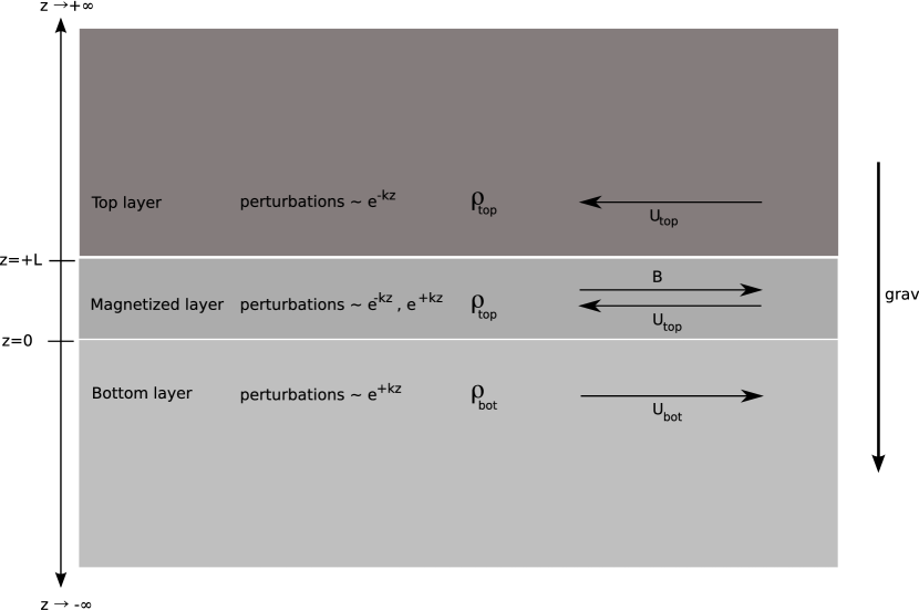
where $x_{i}$ is the $i$-coordinate and can take the values $(x,z)$, $U_{i}$ is the velocity in the $i$-coordinate direction, $\rho$ is density, $\delta\rho$ is any fluctuation in the density, $p$ is pressure, $B$ is the magnetic field, $g$ is the gravitational acceleration with gravity pointing ‘down’ (e.g., in the direction of $-{\bf{\hat{z}}}$). and summation over repeated indicies is implied. We consider velocity, magnetic fields, and pressure of the form

$${\bf{U}} = (u+U,w)\quad u,w\ll U,$$ (5)

$${\bf{B}} = (b_{x}+B,b_{z})\quad b_{x},b_{z}\ll B$$ (6)

where $B$, $W$, and $\rho$ are constant within each region. We will assume that all velocities are highly non-relativistic, so that displacement currents and relativistic effects may be neglected. We also assume that the flow velocities are much less than the sound speed, and thus may consider incompressible flow. A sketch of the situation under consideration is shown in Fig. 1.

Figure 1: A sketch of the problem under consideration. We consider a three-layer problem, with two semi-infinite, uniform, magnetic-field-free regions separated by a layer with a horizontal magnetic field. We consider only field (and disturbances) in the direction of the shear. We will generally consider the magnetized layer to have the same density and velocity as the top fluid. Disturbances are modeled as periodic in the horizontal direction, and vanishing at $\pm\infty$ in the vertical direction.

Following Chandrasekhar (1981) §105, we consider plane wave perturbations of the form $e^{i(kx+nt)}$ for $b_{x},b_{z},u,w,dp,\delta\rho$. Linearizing the equations above results in

$$i\rho\left(n+kU\right)u+\rho U^{\prime}w-\frac{b_{z}}{4\pi}B^{\prime} = -ikdp,$$ (7)

$$i\rho\left(n+kU\right)w-\frac{B}{4\pi}\left(ikb_{z}-b_{x}^{\prime}\right)+\frac{b_{x}}{4\pi\rho}\rho B^{\prime} = dp^{\prime}-g\delta\rho,$$ (8)

$$ib_{x}\left(n+kU\right) = ikBu-wB^{\prime}+b_{z}U^{\prime},$$ (9)

$$ib_{z}\left(n+kU\right) = ikBw,$$ (10)

$$i\delta\rho\left(n+kU\right) = -w\rho^{\prime},$$ (11)

$$iku+w^{\prime} = 0,$$ (12)

$$ikb_{x}+b_{z}^{\prime} = 0.$$ (13)

Because we allow the magnetic field strength to vary between layers, there are extra terms in Eqns. 7,8,9 proportional to $B^{\prime}$ which do not vanish. Within the layers themselves, these terms are identically zero; but their existence will lead to more complex boundary conditions at the interfaces.

2.1 Solution Within Uniform Layers

Equations 9,10,11, and 12 can be solved to express $b_{x},b_{z},b_{x}^{\prime},b_{z}^{\prime},\delta\rho$, and $u$ in terms of $w$ and its derivatives, the system parameters $B,B^{\prime},\rho,\rho^{\prime},U$, the growth rate $n$, and the wavelength of the disturbance $k$. This means that we can begin to write the dispersion relation $n(k)$ in terms of only the perturbed z-velocity $w$ and the known parameters. We can do this by using Eqns. 7 and 8 to eliminate $dp$, and then eliminate all other perturbed variables in favour of $w$, leaving

$$2k\frac{BB^{\prime}}{4\pi\rho}\left(-kwU^{\prime}+\left(n+kU\right)w^{\prime}\right)+$$

$$\left(n+kU\right)^{2}\left(\frac{\rho^{\prime}}{\rho}\left(\frac{gk^{2}w}{\left(n+kU\right)}+U^{\prime}kw-\left(n+kU\right)w^{\prime}\right)+\left(\left(n+kU\right)\left(k^{2}w-w^{\prime\prime}\right)+kwU^{\prime\prime}\right)\right)+$$

$$-\frac{k^{2}}{\left(n+kU\right)}\frac{B^{2}}{4\pi\rho}\left(kw\left(\left(n+kU\right)\left(nk+U^{\prime\prime}\right)+k^{3}U^{2}-2kU^{\prime 2}\right)-\left(n+kU\right)\left(-2kU^{\prime}w^{\prime}+\left(n+kU\right)w^{\prime\prime}\right)\right)=0.$$ (14)

Within the three layers, where $B^{\prime}=0$, $U^{\prime}=0$, and $\rho^{\prime}=0$, we have

$$\left(k^{2}\frac{B^{2}}{4\pi\rho}-\left(n+kU\right)^{2}\right)\left(k^{2}w-w^{\prime\prime}\right)=0$$ (15)

which, since we are only interested in negative $n^{2}$, leaves us with only the solutions

$$w(z)\sim e^{+kz},\quad w(z)\sim e^{-kz}$$ (16)

as in the case of uniform field, and as anticipated in Fig. 1.

2.2 Boundary Conditions Between Layers

The normal displacement of the interface is $-iw/(n+kU)$; this can be seen by expressing the perturbed interface position $\delta z$ in the same form of the other perturbed variables, and the linear-order evolution equation for $\delta z$ becomes, $i(n+kU)\delta z=w$.

Because the displacement of the interface must be unique, $w/(n+kU)$ must be continuous across the interfaces. This and a related quantity, the shifted time derivative $(n+kU)$ occurs frequently enough that it is useful to express Eq. 14 in terms of these quantities. Doing so results in

$$-2\left(n+kU\right)^{\prime}\left(\frac{w}{n+kU}\right)^{\prime}\left(n+kU\right)\rho+\left(\frac{w}{n+kU}\right)^{\prime\prime}\left(k^{2}\frac{B^{2}}{4\pi}-\left(n+kU\right)^{2}\rho\right)$$

$$-k^{4}\frac{B^{2}}{4\pi}\left(\frac{w}{n+kU}\right)+k^{2}\left(n+kU\right)^{2}\rho\left(\frac{w}{n+kU}\right)+2k^{2}\left(\frac{w}{n+kU}\right)^{\prime}\frac{BB^{\prime}}{4\pi}-$$

$$\left(\frac{w}{n+kU}\right)^{\prime}\left(n+kU\right)^{2}\rho^{\prime}+gk^{2}\left(\frac{w}{n+kU}\right)\rho^{\prime}=0$$ (17)

Integrating this equation over an infinitesimal region across either of the interfaces gives us the boundary conditions across this interface. In doing so, terms that contain no derivatives vanish in the limit, and we are left with

$$gk^{2}\left[\rho\right]\left.\left(\frac{w}{n+kU}\right)\right|_{i}-\left[\rho\left(n+kU\right)^{2}\left(\frac{w^{\prime}}{n+kU}\right)\right]+k^{2}\left[\frac{B^{2}}{4\pi}\left(\frac{w^{\prime}}{n+kU}\right)\right]=0$$ (18)

where $[f]$ indicates the jump in a quantity $f$ across the interface, and a subscript $i$ refers to a value at the interface. Note that when $B$ is constant, this reduces exactly to the homogeneous field case found in Chandrasekhar (1981) §106.

2.3 Matching the Solutions

In the top and bottom layer, one of the two solution branches ($w\sim\exp{(+kz)}$ and $w\sim\exp{(-kz)}$, respectively) are clearly unphysical. In the middle layer, however, both can coexist, and so we have as forms for the solutions

$$w=\left\{\begin{array}[]{ll}w_{3}e^{-kz}&\mathrm{top\,layer}\\ w_{2+}e^{+kz}+w_{2-}e^{-kz}&\mathrm{middle\,layer}\\ w_{1}e^{+kz}&\mathrm{bottom\,layer}\end{array}\right.$$ (19)

Because $w/(n+kU)$ must be continuous across the interface, we have

$$\frac{w_{1}}{\left(n+kU\right)} = \frac{w_{2+}+w_{2-}}{\left(n-kU\right)},$$ (20)

$$\frac{w_{3}e^{-kl}}{\left(n-kU\right)} = \frac{w_{2+}e^{+kl}+w_{2-}e^{-kl}}{\left(n-kU\right)}.$$ (21)

These can be solved for the components of the intermediate velocity in terms of the outer layer velocities, giving

$$w_{2+} = \frac{w_{1}\left(n-kU\right)-w_{3}\left(n+kU\right)}{(e^{2kl}-1)(n+kU)},$$ (22)

$$w_{2-} = \frac{w_{1}e^{2kl}(n-kU)-w_{3}(n+kU)}{(e^{2kl}-1)(n+kU)}.$$ (23)

$$\left(\frac{w}{n+kU}\right)^{\prime}_{2,z=l} = w_{1}k\frac{e^{kl}}{e^{2kl}-1}\frac{-n+kU}{n-kU}+w_{3}k\frac{e^{-kl}\left(e^{2kl}+1\right)}{e^{2kl}-1}$$ (24)

$$\left(\frac{w}{n+kU}\right)^{\prime}_{2,z=0} = 2w_{1}k\frac{e^{2kl}+1}{e^{2kl}-1}\frac{-n+kU}{n+kU}+2w_{3}k\frac{1}{e^{2kl}-1}$$ (25)

We now have two boundary conditions to satisfy — Eq. 18 at the two interfaces between the layers.

The top interface condition gives us

$$\rho_{\mathrm{top}}\left(w_{3}k+\left(n-kU\right)\left(\frac{w}{n+kU}\right)^{\prime}_{2,z=l}\right)-k^{2}\frac{B^{2}}{4\pi}\left(\frac{w}{n+kU}\right)^{\prime}_{2,z=l}=0$$ (26)

and the bottom interface gives us

$$gk^{2}\left(\rho_{\mathrm{top}}-\rho_{\mathrm{bot}}\right)\frac{w_{1}}{\left(n+kU\right)}-\left(\rho_{\mathrm{top}}\left(n-kU\right)\left(\frac{w}{n+kU}\right)^{\prime}_{2,z=0}-\rho_{\mathrm{bot}}w_{1}k\right)+k^{2}\frac{B^{2}}{4\pi}\left(\frac{w}{n+kU}\right)^{\prime}_{2,z=0}=0$$ (27)

This gives us two equations in terms of $w_{1}$ and $w_{3}$. Using our expressions for $w_{2\pm}$ and then solving the first equation for $w_{3}$ in terms of $w_{1}$ and substituting the result into the second gives us our final dispersion relation of

$$\left[n^{2}+k^{2}U^{2}+\mathrm{At}k\left(g-2nU\right)\right] +$$

$$\left(e^{2kl}-1\right)\frac{\left(\left(n-kU\right)^{2}-\frac{1}{2}k^{2}v_{A}^{2}\right)\left(n^{2}+k^{2}U^{2}+\mathrm{At}k\left(g-2nU\right)-\frac{1+\mathrm{At}}{2}k^{2}v_{A}^{2}\right)}{\left(n-kU\right)^{2}-k^{2}v_{A}^{2}} = 0$$ (28)

where the Atwood number, $\mathrm{At}$, is defined to be the non-dimensional density difference

$$\mathrm{At}=\frac{\rho_{\mathrm{top}}-\rho_{\mathrm{bot}}}{\rho_{\mathrm{top}}+\rho_{\mathrm{bot}}}.$$ (29)

It is worth noting that in the no magnetization limit $v_{A}\rightarrow 0$, the only term containing $l$ can be divided out, so that the solution does not depend on $l$; this is as it must be, as without a magnetic field nothing distinguishes the $l$-thick middle layer from the top layer. Also, in the infinitely thin layer limit $\exp{2kl}\rightarrow 1$ and the solution reduces to the non-magnetized case.

3 EFFECT ON THE RAYLEIGH-TAYLOR INSTABILITY

If we consider the ‘pure’ Rayleigh-Taylor instability, with no horizontal shear, then $U\rightarrow 0$ and we are left with

$$n^{2}+\mathrm{At}gk+\left(e^{2kl}-1\right)\frac{\left(n^{2}-\frac{1}{2}k^{2}v_{A}^{2}\right)\left(n^{2}+\mathrm{At}gk-\frac{1+\mathrm{At}}{2}k^{2}v_{A}^{2}\right)}{n^{2}-k^{2}v_{A}^{2}}=0.$$ (30)

This equation relates the growth rate $n$ to two other inverse timescales on the scale of $k^{-1}$ – an Alfvén frequency $\omega_{A}^{2}=k^{2}v_{A}^{2}$, and a gravitational timescale $\tau_{g}^{-2}=\mathrm{At}gk$. Expressing the growth rate and Alfvén frequency in units of the inverse gravitational timescale, and ignoring the trivial Alfvén wave solution $n=\omega_{A}$, the result is a quadratic in $n^{2}$:

$$e^{2kl}\tilde{n}^{4}+\left(\left(1-\omega_{A}^{2}\right)+\left(e^{2kl}-1\right)\left(1-\frac{2+\mathrm{At}}{2}\omega_{A}^{2}\right)\right)\tilde{n}^{2}-\omega_{A}^{2}\left(1+\frac{1}{2}\left(e^{2kl}-1\right)\left(1-\frac{1+\mathrm{At}}{2}\omega_{A}^{2}\right)\right)=0.$$ (31)

To consider the degree to which the magnetized layer stabilizes against the Rayleigh-Taylor instability, we consider (for simplicity) the maximally unstable case where $\mathrm{At}\rightarrow 1$. For stability, it is necessary and sufficient that the roots of the quadratic in $n^{2}$ be positive and real; a quadratic of the form $ax^{2}+bx+c=0$ has positive and real roots for $c/a>0$, $b/a<0$, and $b^{2}-4ac>0$. The first two of these conditions reduce to

$$\omega_{A}^{2} > \frac{e^{2kl}+1}{e^{2kl}-1}$$ (32)

$$\omega_{A}^{2} > \frac{2e^{2kl}}{3e^{2kl}-1},$$ (33)

and the third is satisfied for all real $\omega_{A}^{2}$. Of these conditions, the first controls, as the second simply posts a lower limit for $\omega_{A}^{2}$ of between $2/3$ and $1$, while the lower limit for the first is always greater than $1$. Thus the condition for stability in the case of a Rayleigh-Taylor instability with $\mathrm{At}=1$, which would otherwise always be unstable, is

$$v_{A}^{2}>\left(\frac{e^{2kl}+1}{e^{2kl}-1}\right)gk^{-1}$$ (34)

with no strength of magnetic field able to stabilize in the case of an infinitely thin layer. This stability criterion is shown in Fig 2.

Figure 2: Plotted is the Rayleigh-Taylor stability boundary for the most-unstable ($\mathrm{At}=1$) case, as given in Eq. 34. The magnetic field strength in the magnetized layer (here expressed as the Alfvén speed squared in units of $g/k$) necessary to stabilize against a mode is plotted as a function of the thickness of the layer in units of the wavelength of the mode. Thus, to stabilize modes an order of magnitude greater longer than the layer is thick ($l/\lambda\approx 0.1$), a magnetic field such that $v_{A}^{2}\gtrsim 2g/k$ is necessary.

4 EFFECT ON THE KELVIN-HELMHOLTZ INSTABILITY

The shear terms in the case of the Kelvin-Helmholtz instability make the dispersion relation significantly more complicated,

$$n^{4}-2\left(1+\mathrm{At}\right)kUn^{3}+\frac{1}{2}e^{-2kl}\left(\mathrm{At}k^{2}v_{A}^{2}+e^{2kl}\left(4\left(1+2\mathrm{At}\right)k^{2}U^{2}-(2+\mathrm{At})k^{2}v_{A}^{2}\right)\right)n^{2}+$$

$$-e^{-2kl}kU\left(k^{2}v_{A}^{2}+e^{2kl}\left(2(1+\mathrm{At})k^{2}U^{2}-(1+2\mathrm{At})k^{2}V_{A}^{2}\right)\right)n+$$

$$\frac{1}{4}e^{-2kl}\left(2\mathrm{At}k^{2}U^{2}k^{2}v_{A}^{2}-\left(1+\mathrm{At}\right)k^{4}v_{A}^{4}+e^{2kl}\left(2k^{2}U^{2}-k^{2}v_{A}^{2}\right)\left(2k^{2}U^{2}-\left(1+\mathrm{At}\right)k^{2}v_{A}^{2}\right)\right) = 0.$$ (35)

For considering the stability boundary we will again consider the most unstable case, in this case $\mathrm{At}=0$. As in the previous case, the growth rate and the Alfvén frequency can be expressed in terms of the other timescale of the problem, the advection time across the wavelength of the perturbation, $\tau_{U}=1/(kU)$, leaving us with

$$\tilde{n}^{4}-2\tilde{n}^{3}-\left(\omega_{A}^{2}-2\right)\tilde{n}^{2}+\left(\omega_{A}^{2}\left(1-e^{-2kl}\right)-2\right)\tilde{n}$$

$$+\frac{1}{4}\left(\left(\omega_{A}^{2}-2\right)^{2}-\omega_{A}^{4}e^{-2kl}\right) = 0.$$ (36)

While this is a fairly unpleasant quartic in $n$, it is a fairly approachable quadratic in $\omega_{A}^{2}$:

$$\frac{1}{4}\left(e^{2kl}-1\right)\omega_{A}^{4}+\left(1+\tilde{n}\left(e^{-2kl}-1\right)+\tilde{n}^{2}\right)\omega_{A}^{2}-(\tilde{n}-1)^{2}(\tilde{n}^{2}+1)=0.$$ (37)

The two roots are

$$\omega_{A}^{2}=2\frac{\tilde{n}+e^{2kl}+(\tilde{n}-1)ne^{2kl}\pm\sqrt{\left(\tilde{n}^{2}+e^{2kl}\right)\left(1+\tilde{n}^{2}e^{2kl}\right)}}{e^{2kl}-1}.$$ (38)

For stability, we consider the neighborhood around $Im(\tilde{n})=0$. In this case, both these branches have minima for purely oscillatory modes around $\tilde{n}=1$; but in this neighborhood the second, negative, branch, has no real solutions for $\omega_{A}$ with $Im(\tilde{n})\neq 0$, so cannot be relevant to the question of stability. The positive branch has a minimum of

$$\omega_{A}^{2}=4\frac{e^{2kl}+1}{e^{2kl}-1}$$ (39)

so that stability is ensured when this condition is met, or

$$v_{A}^{2}\geq\left(\frac{e^{2kl}+1}{e^{2kl}-1}\right)(2U)^{2},$$ (40)

which is the same condition for stability of the Rayleigh-Taylor instability, but with $2U$ replacing $g/k$; recall, however, that the two conditions are for two different values of the Atwood number, such that the instability is maximized in each case. This stability criterion is plotted in Fig. 3.

Figure 3: Plotted is the Kelvin-Helmholtz stability boundary for the most-unstable ($\mathrm{At}=1$) case, as given in Eq. 40. The magnetic field strength in the magnetized layer (here expressed as the Alfvén speed squared in units of the half-shear velocity squared, $U^{2}$) necessary to stabilize against a mode is plotted as a function of the thickness of the layer in units of the wavelength of the mode. Thus, to stabilize modes an order of magnitude greater longer than the layer is thick ($l/\lambda\approx 0.1$), a magnetic field such that $v_{A}^{2}\gtrsim 2(2U)^{2}$ is necessary.

5 NUMERICAL RESULTS

To confirm the results of the previous sections, numerical experiments were performed in two dimensions using version 3.0 of the Athena code (Gardiner and Stone, 2005), a dimensionally unsplit, highly configurable MHD code. For the results in this work we used the ideal gas MHD solver with an adiabatic equation of state ($\gamma=1.4$), and the 3rd-order accurate solver using a Roe-type flux function. We considered a domain of size, in code units, of $[-1/6,1/6]\times[-1/6,1/6]$ with resolution $400\times 400$ for the Kelvin-Helmholtz instability simulations, and with a slightly vertically extended domain ($[-1/6,1/6]\times[-1/4,1/4]$, $400\times 600$) for the Rayleigh-Taylor instability experiments.

To ensure that the resolution used was adequate, a resolution study was performed on a fiducial run (a Rayleigh-Taylor simulation with $B_{x,0}=0.07,v_{A}=0.0495$; the magnetic field code units are such that the Alfvén speed, $v_{A}^{2}=B^{2}/2$) with resolution varying between a factor of two less than this resolution and a factor of two more; measured growth rates varied by only approximately $\pm 3$ percent.

The analytic results presented in previous sections were in the incompressible limit; in our numerical experiments here the fiducial density was $1$ in code units and the pressure was set so that the sound speed $c_{s}$ would be $1$ in code units, which is an order of magnitude larger than the velocities achieved in either set of simulations; thus the Mach number ${\cal{M}}<0.1$, and incompressibility remains a reasonable approximation. In both set of simulations, a magnetized layer of thickness $1/60$ was initialized starting at $y=0$, with strength of magnetic field varied from run to run. To keep the initial conditions in pressure equilibrium, the thermal pressure was reduced in this layer, but because of the large sound speed (and consequently large plasma $\beta$) this was a small reduction (never more than a few percent).

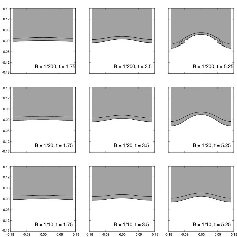
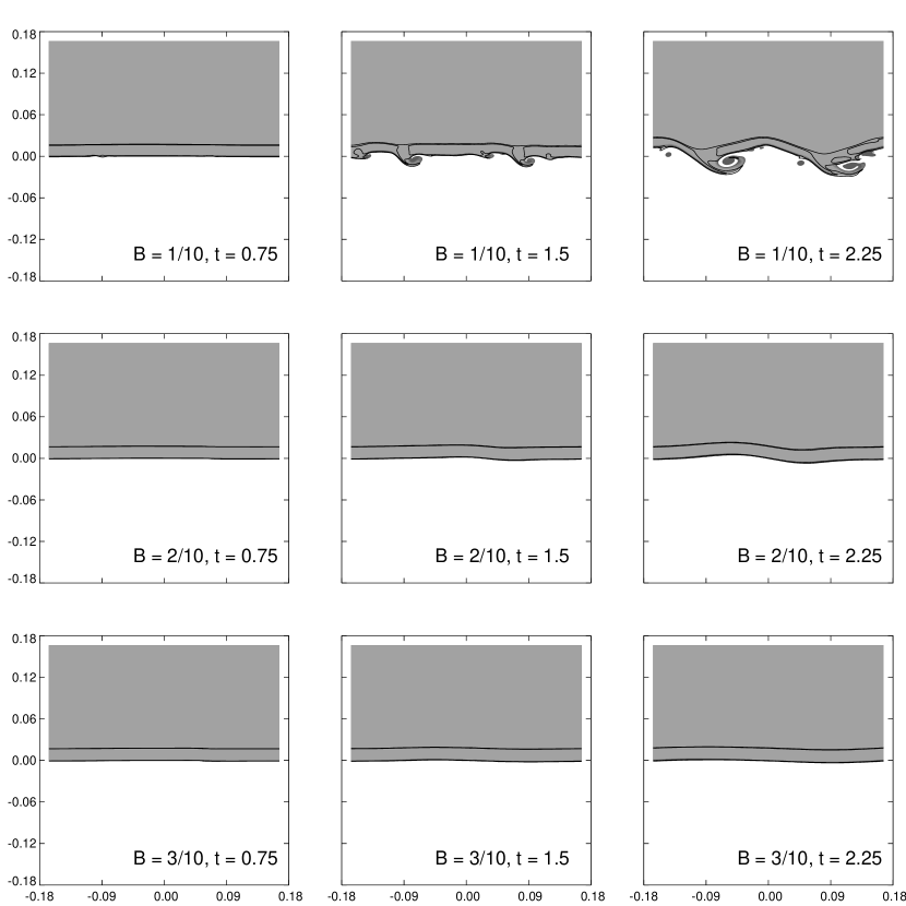
In both sets of simulations, the interface was given a sinusoidal velocity with a wavelength equal to the size of the box, and an amplitude of $v_{pert}\approx 0.0025$. In the Kelvin-Helmholtz case, a background shear velocity of $-0.1$ in the $x$ direction was applied to the top layer and the magnetized layer, and of $+0.1$ in the bottom layer. In the Rayleigh-Taylor case, a gravitational acceleration of $g=0.1$ was applied in the negative $y$ direction. Both set of simulations used an Atwood number $\mathrm{At}=1/3$, so that the top layer had density $\rho_{t}=2$. Snapshots of the evolution of the simulations are shown in Figs.4 and 5.

Figure 4: Snapshots from representative runs of the Rayleigh-Taylor instability with a magnetized layer, performed with the Athena code. Shading represents density, and contours indicate magnetic field strength. In code units, the density of the top fluid is $\rho_{t}=2$, and that of the bottom is $\rho_{t}=1$ ($\mathrm{At}=1/3$), and pressure is set such that in the bottom layer the adiabatic sound speed $c_{s}$ is 10, and the domain is in total pressure equilibrium. The wavelength of the initial perturbation is $1/3$, and the thickness of the magnetized layer is $1/60$; the acceleration due to gravity $g$ is $1/10$ and in the negative $y$ direction. Shown are runs with varying initial horizontal magnetic fields, with, from top to bottom, $B_{x,0}=1/200,1/20,1/10$. Snapshots are shown at times in code units of, left to right, approximately $(1.75,3.5,5.25)$. The contours are for magnetic field strength of $B_{x,0}/4$ and $3B_{x,0}/4$.

Figure 5: Snapshots from representative runs of the Kelvin-Helmholtz instability with a magnetized layer, performed with the Athena code. Shading represents density, and contours indicate magnetic field strength. In code units, the density of the top fluid is $\rho_{t}=2$, and that of the bottom is $\rho_{t}=1$ ($\mathrm{At}=1/3$), and pressure is set such that in the bottom layer the adiabatic sound speed $c_{s}$ is 1, and the domain is in total pressure equilibrium. The wavelength of the initial perturbation is $1/3$, and the thickness of the magnetized layer is $1/60$; the acceleration due to gravity $g$ is $1/10$ and in the negative $y$ direction. Shown are runs with varying initial horizontal magnetic fields, with, from top to bottom, $B_{x,0}=0.1,0.2,0.3$. Snapshots are shown at times in code units of, left to right, approximately $(0.75,1.5,2.25)$. The contours are for magnetic field strength of $B_{x,0}/4$ and $3B_{x,0}/4$.

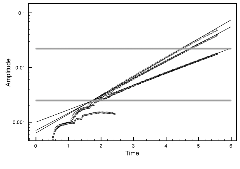
From the outputs of the simulations, growth rates for the instabilities were calculated by considering the growth of the amplitude (measured by finding the mean vertical position of the magnetized layer and fitting to a sinusoid of the wavelength of the perturbed mode) as a function of time. Exponentials were fit to this series of amplitudes, for those times where the amplitude was resolved by at least three zones and where the amplitude was less than $1/15$ of the wavelength (e.g., before nonlinear evolution begins to matter). For the simulations reported here, this means the fit was performed with amplitudes in the range $[1/400,1/45]$, covering approximately a decade in amplitude. Plotted in Fig. 6 are four examples of this procedure for the Rayleigh-Taylor simulations. For comparison, the results of a resolution study of a fiducial Rayleigh-Taylor case is shown in Fig. 7.

Figure 6: Evolution of amplitude of the Rayleigh-Taylor perturbation with time, for several runs (plotted are, top to bottom, $B_{0}=(0.005,0.05,0.1,0.2)$), shown as symbols; also plotted here are best-fit exponentials to measure the growth rate of the instability. Exponentials were fit to data from those times where the amplitude was resolved by at least three zones and where the amplitude was less than $1/15$ of the wavelength (e.g., before nonlinear evolution begins to matter); for the simulations reported here, this means the fit was performed with amplitudes in the range $[1/400,1/45]$, covering approximately a decade in amplitude. The range considered is indicated by thick shaded lines; below the bottom line the ‘jumpiness’ due to poor resolution on the grid is visible, and above deviations from exponential behaviour due to nonlinear effects becomes evident.

Figure 7: As in Figure 6, but with $B_{0}=0.07$, and varying the resolution. Shown are for several runs with $N$ varying by a factor of $4$, where $N$ is the horizontal resolution in the simulation, with vertical resolution kept proportionate; thus N is the number of points used to represent one wavelength, with the thickness of the layer being represented by $N/20$ points. $N=100$ is not quite enough resolution to accurately measure the growth rate, but the difference in fitted exponential growth rates between $200$, $400$, $600$, and $800$ is only a few percent.

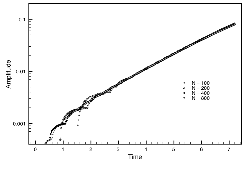
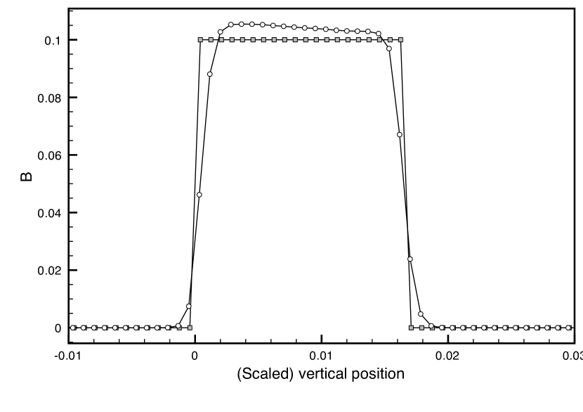
Because of the low speeds of these flows, many timesteps (typically on order 20000) must be take to evolve these instabilities. Over that period of time modest amounts of numerical diffusion slightly modify the structure of the magnetic layer, as does the still slightly compressible flow itself; the change is shown in Fig.8. The growth rate of the instabilities is very sensitive to the thickness of the layer, and this modification of the magnetic layers thickness must be taken into account when comparing with analytic results.

Figure 8: Magnetic field profile through $x=0$ for the $B_{x,0}=1/10$ Rayleigh-Taylor simulation at time 0 (filled squares) and 3.75 (open circles). The later-time profile is shifted leftwards by $\delta y=0.00675$ for comparison. During the course of the simulation, the thickness of the magnetic field layer at its peak is reduced to about 18 grid points from the original 20. Besides the inevitable effects of numerical diffusion slightly smearing out the profile over approximately 18000 timesteps, effects from the slight compressibility of the flow, and asymmetry from the direction of gravity (to the left in this plot) is shown by the slight increase in magnetic field density and the slope at late times.

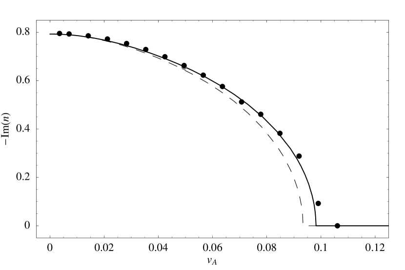
The comparison of measured growth rates to analytic results is shown in Figs. 9 and 10, with theoretical results taken from the numerical solution of Eqs. 30 and 35. Where the numerical experiments can give clean growth rate measurements, the analytic and numerical results agree to within a few percent, and there is also agreement at the few percent level on the boundary of stability.

Figure 9: Rayleigh-Taylor growth rates as a function of magnetic field strength (given here in terms of Alfvén speed, $v_{A}$) in the magnetized layer, measured from simulation (diamonds) and predicted from analytic theory (lines). The dashed line gives the prediction using the nominal width of the magnetized field layer, and the solid line gives the prediction for the actual width of the magnetized layer in the simulations after diffusion eats away at the profile as shown in Fig. 8. A gray point indicates a run done at twice the resolution to check to see if the default resolution was adequate. The theoretical curves are taken from numerical solution of the dispersion relation, Eq. 30.

Figure 10: Kelvin-Helmholtz growth rates as a function of magnetic field strength (given here in terms of Alfvén speed, $v_{A}$) in the magnetized layer, measured from simulation (diamonds) and predicted from analytic theory (lines). The dashed line gives the prediction using the nominal width of the magnetized field layer, and the solid line gives the prediction for the actual width of the magnetized layer in the simulations after diffusion eats away at the profile as shown in Fig. 8. Below $v_{A}\approx 0.1$, smaller-wavelength modes, seeded by numerical grid noise, grow very quickly and contaminate any attempt to measure a linear growth rate for the mode under consideration. The theoretical curves are taken from numerical solution of the dispersion relation, Eq. 35.

6 DISCUSSION

We have shown, through derivation of dispersion relations and two-dimensional numerical experiments, that it is possible for even thin magnetized layers to suppress instability growth on scales much larger than their own thickness as long as the magnetic field strength is high enough that the Alfvén velocity in the layer in the direction of the perturbation is of order the relevant destabilizing velocity scales. In the case of the Kelvin-Helmholtz instability, the most most relevant case for core mergers, a magnetized layer can stabilize modes an order of magnitude larger than the thickness of the layer if the Alfvén speed of the same magnitude as the full shear velocity $v_{A}\approx 2U$. But this is almost automatically true; as shown in Lyutikov (2006), near the stagnation line the magnetic pressure reaches equipartition with the ram pressure, meaning that this condition on the velocities is met. Thus we would expect, certainly near the stagnation line, that the magnetic draping ‘protects’ a merging core from instabilities, as would appear to be the case in simulations published in the literature (Asai et al., 2004, 2005, 2006, Dursi and Pfrommer, in preparation).

Clearly, this stabilization only applies to perturbations along the field; but in this plane, then, the draped field can then have the twin effects of protecting the merging core against thermal disruption, and reducing the shear effects which would tend to mix in the core material earlier. In the plane perpendicular to the magnetic field, shear-driven instability will occur unimpeded, leading to a distinct asymmetry in the resulting magnetic layer and, presumably, the moving core or bubble. Such asymmetries have been seen in 3d simulations in the literature, as cited above, and would potentially be observable. It is interesting to note however that even a quite weak field can effect global mixing in the presence of similar instabilities (e.g., Gardiner and Stone, 2007), and so even in the plane perpendicular to the field it is possible that a thin magnetized layer could keep an interface sharper than could exist absent the magnetic field.

The full three dimensional stability problem remains to be tackled, and less clear still is the effect of a more realistic magnetic field, not expected to be planar or uniform, and the effects of fully three-dimensional perturbations on such a layer. Consideration of this more complicated and realistic case is left to future work.

References

- Asai et al. [2004] N. Asai, N. Fukuda, and R. Matsumoto. MHD Simulations of a Moving Subclump with Heat Conduction. Journal of Korean Astronomical Society, 37:575–578, December 2004.
- Asai et al. [2005] N. Asai, N. Fukuda, and R. Matsumoto. Three-dimensional MHD simulations of X-ray emitting subcluster plasmas in cluster of galaxies. Advances in Space Research, 36:636–642, 2005. 10.1016/j.asr.2005.04.041.
- Asai et al. [2006] N. Asai, N. Fukuda, and R. Matsumoto. MHD simulations of plasma heating in clusters of galaxies. Astronomische Nachrichten, 327:605–+, June 2006. 10.1002/asna.200610601.
- Bernikov and Semenov [1980] L. V. Bernikov and V. S. Semenov. Problem of MHD flow around the magnetosphere. Geomagnetizm i Aeronomiia, 19:671–675, February 1980.
- Bîrzan et al. [2004] L. Bîrzan, D. A. Rafferty, B. R. McNamara, M. W. Wise, and P. E. J. Nulsen. A Systematic Study of Radio-induced X-Ray Cavities in Clusters, Groups, and Galaxies. ApJ, 607:800–809, June 2004. 10.1086/383519.
- Chandrasekhar [1981] S. Chandrasekhar. Hydrodynamic and Hydromagnetic Stability. Dover, New York, 1981.
- Ettori and Fabian [2000] S. Ettori and A. C. Fabian. Chandra constraints on the thermal conduction in the intracluster plasma of A2142. MNRAS, 317:L57–L59, September 2000.
- Gardiner and Stone [2005] T. A. Gardiner and J. M. Stone. An unsplit Godunov method for ideal MHD via constrained transport. Journal of Computational Physics, 205:509–539, May 2005. 10.1016/j.jcp.2004.11.016.
- Gardiner and Stone [2007] T. A. Gardiner and J. M. Stone. Nonlinear Evolution of the Magnetohydrodynamic Rayleigh-Taylor Instability. 1022, July 2007.
- Lyutikov [2006] M. Lyutikov. Magnetic draping of merging cores and radio bubbles in clusters of galaxies. MNRAS, 373:73–78, November 2006. 10.1111/j.1365-2966.2006.10835.x.
- Markevitch and Vikhlinin [2007] M. Markevitch and A. Vikhlinin. Shocks and cold fronts in galaxy clusters. Phys. Rep., 443:1–53, May 2007. 10.1016/j.physrep.2007.01.001.
- McNamara et al. [2005] B. R. McNamara, P. E. J. Nulsen, M. W. Wise, D. A. Rafferty, C. Carilli, C. L. Sarazin, and E. L. Blanton. The heating of gas in a galaxy cluster by X-ray cavities and large-scale shock fronts. Nature, 433:45–47, January 2005. 10.1038/nature03202.
- Robinson et al. [2004] K. Robinson, L. J. Dursi, P. M. Ricker, R. Rosner, A. C. Calder, M. Zingale, J. W. Truran, T. Linde, A. Caceres, B. Fryxell, K. Olson, K. Riley, A. Siegel, and N. Vladimirova. Morphology of Rising Hydrodynamic and Magnetohydrodynamic Bubbles from Numerical Simulations. ApJ, 601:621–643, February 2004. 10.1086/380817.
- Ruszkowski et al. [2007a] M. Ruszkowski, T. A. Ensslin, M. Bruggen, M. C. Begelman, and E. Churazov. Cosmic ray confinement in fossil cluster bubbles. ArXiv e-prints, 705, May 2007a.
- Ruszkowski et al. [2007b] M. Ruszkowski, T. A. Enßlin, M. Brüggen, S. Heinz, and C. Pfrommer. Impact of tangled magnetic fields on fossil radio bubbles. MNRAS, pages 400–+, May 2007b. 10.1111/j.1365-2966.2007.11801.x.
- Vikhlinin et al. [2001] A. Vikhlinin, M. Markevitch, and S. S. Murray. A Moving Cold Front in the Intergalactic Medium of A3667. ApJ, 551:160–171, April 2001. 10.1086/320078.