The Emerging Features of Bipolar Magnetic Regions during Solar Minima

Abstract

Solar magnetic synoptic charts obtained by NSO/Kitt Peak and SOHO/MDI are analyzed for studying the appearance of bipolar magnetic regions (BMRs) during solar minima. As a result, we find the emergence of long-lived BMRs has three typical features. (1) BMRs’ emerging rates of the new cycles increase about 3 times faster than those of the old cycles decrease. (2) Two consecutive solar cycles have an overlapping period of near 10 Carrington rotations. During this very short overlapping time interval, BMRs of two cycles tend to concentrate in the same longitudes. (3) About 53% BMRs distribute with a longitudinal distance of 1/8 solar rotation. Such phenomenon suggests a longitudinal mode of $m=8$ existing during solar minima.

1 Introduction

New magnetic flux of the sun always appears as a bipolar magnetic region (BMR) from below in form of two distinct types. One is the emerging flux region (EFR), the other is the ephemeral region (ER). EFR is an important ingredient in active region fields which sometimes can be seen as large-scale patterns, e.g. active longitudes defined as a sequence of active regions appearing in the preferred longitudinal bands (Gaizauskas et al. 1983). ER is relatively small and short-lived (about 1 day), thus it distributes more randomly. In this paper, using solar magnetic synoptic charts we investigate patterns in emergence of the long-lived (at least 1 rotation) BMRs during solar activity minima. The emergence of BMRs during solar minima is a very classical topic, addressed by many people, e.g. Howard & LaBonte 1981, Howard 1989, Wang & Sheeley 1989, Harvey & Zwaan 1993, and many others. Differing from former works, here more attention is paid to the variability of BMRs’ emerging rate and the typical longitudinal distance among them. It is believed that such information can provide hints for understanding the origin of solar magnetic fields.

2 Data Processing

As the main source of data, we have used NSO/Kitt Peak solar magnetic synoptic charts and SOHO/MDI synoptic charts. For our purpose we choose three time intervals of solar minima: Carrington rotation (CR) 1754-1793, CR1891-1930 and CR2035-2049. During the former two time intervals we use Kitt Peak synoptic charts and during the last time interval, we use SOHO/MDI charts since Kitt Peak charts are not available after CR2007. When dealing with the high resolution SOHO/MDI charts, we resized the grid from $3600\times 1080$ to the Kitt Peak’s grid $360\times 180$.

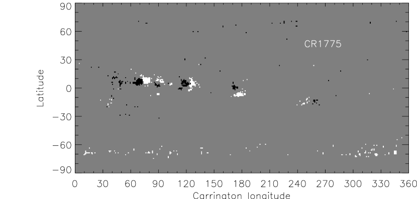
Figure 1: The NSO/Kitt Peak solar magnetic synoptic chart of CR1775. Its original sine latitude is re-mapped into an equal latitude by using a linear interpolation method, and the pixels with absolute value lower than 20 Gauss are set to zero.

To identify BMRs in each solar magnetic synoptic chart, we set three criteria. (1) A BMR should possess strong magnetic fields. Here all pixels with absolute value lower than 20 Gauss are set to zero (see an example in Figure 1) because they are thought to be related to the quiet sun and network magnetic fields (Rabin et al., 1991). (2) BMR’s two polarities should distribute closely and weight balanced; (3) It should do not exist in the former CR and leave an obvious track in the following CR. Therefore the BMRs chosen for every CR should be new and long-lived. Also for this reason, the statistic of BMRs’ distribution won’t be affected by the evolution of the relatively random ERs. After finding a BMR, we outline its region and calculate its absolute flux gravity center. In order to cut down the latitudinal measurement errors, we have used a linear interpolation method to re-map synoptic charts’ sine latitude into equal latitude. As shown in Figure 2, all BMRs found during CR1906-1925 are signed together by circles. The center of circle marks the BMR’s flux gravity center (or BMR’s position).

3 Results and Discussion

Figure 3 depicts the latitudinal distribution of solar emerging BMRs during the three chosen time intervals (CR1754-1793, CR1891-1930 and CR2035-2049). According to the Spörer law we can easily draw the separatrix between the old and new solar cycles. Here we can see clearly that there is a very special BMR (see the arrow in Figure 3). Following the discussion of de Toma et al. (2000), we also think this BMR belongs to cycle 23 and just emerged much earlier.

3.1 BMRs’ Emerging Rate

BMRs’ emerging rates (the number of new BMRs per CR) during each solar cycles are computed. The result is shown in the left panel of Figure 4 where the solid lines indicate BMRs of the old solar cycles and the dashed lines indicate BMRs of the new solar cycles. Using a least-square linear fit, we find the BMRs’ emerging rates during the end of cycles 21, 22 descend at an average rate of $0.052\pm 0.016$ $CR^{-2}$ and $0.089\pm 0.020$ $CR^{-2}$, while the emerging rates ascend at a rate of $0.168\pm 0.059$ $CR^{-2}$ and $0.225\pm 0.077$ $CR^{-2}$ during the beginning of cycles 22, 23 (regardless of the special BMR mentioned in the above paragraph). Therefore BMRs’ emerging rates of new cycles increase about 3 times faster than those of old cycles decrease. The right panel of Figure 4 shows the sunspot number during the same time intervals. We find the sunspot curves in the right panel are very similar to the BMR curves in the left panel. Some local differences mainly come from the fact we only compute the new BMRs during each CR.

Figure 3 and Figures 4a, 4b show that two consecutive solar cycles overlap about 10 CRs. During such overlapping period the BMRs’ emerging rate gets the least. Table 1 lists the longitudes of BMRs occurring during the overlapping time interval of cycles 21, 22 and cycles 22, 23. From this we can find that most BMRs of the old and new cycles tend to concentrate in the same longitudes. Bumba et al. (2000) also found this phenomenon and suggested this would be due to the magnetic flux of the new cycle induced by the action of the old cycle magnetic flux.

3.2 Longitudinal Distance among BMRs

We mainly study the longitudinal distance ($d=|l_{A}-l_{B}|$, $l$ means the BMR’s Carrington longitude) between every two BMRs of the same cycle, emerging in the same CR or $\pm 1$ CR ($|\vartriangle{t}|\leq 1$ $CR$, $t$ means the BMR’s emerging time), and with a latitudinal distance of no more than $8^{\circ}$ ($|\vartriangle{\theta}|\leq 8^{\circ}$, $\theta$ means the BMR’s latitude). Only two BMRs satisfying such three conditions can be called one BMR pair. Here we totally find 155 qualified BMR pairs. Due to the spherical solar surface, each BMR pairs’ longitudinal distance $d$ should be also regarded as $360^{\circ}-d$ (the unit of $d$ is $1^{\circ}$). Therefore, we add the number of BMR pairs with a distance $d$ and $360^{\circ}-d$. The final result is shown by the dashed line in Figure 5 (for the bilateral symmetry, we just draw the former half $d\in[0^{\circ},180^{\circ}]$). With a measurement of its smoothing effect (see the solid line in Figure 5), we find 82 (or 53%) BMR pairs to distribute near (peak width at half-height, $\sigma^{\pm}\in[4^{\circ},11^{\circ}]$, see Figure 5) four typical longitudinal distances: $d=49^{\circ}$, $d=95^{\circ}$, $d=136^{\circ}$, and $d=178^{\circ}$. There is another distinct peak located at around $d=20^{\circ}$. Such $d$ is so small that we think it might originate from BMRs’ mutual action (e.g. while a BMR emerging within another existing BMR, they may compete for place with each other) or the differential rotation. In order to further check up our result, we have carried out similar study for the new/old solar cycle and the northern/southern hemisphere separately, only to find that the peak positions are the same.

Very regular four peak positions, $d=49^{\circ}$, $d=95^{\circ}$, $d=136^{\circ}$, and $d=178^{\circ}$, are separated up to multiples of $45^{\circ}$. This phenomenon indicates that most BMRs tend to distribute with a longitudinal distance of 1/8 solar rotation. We think such rule should be related to the quantified distribution of solar magnetic field. Gilman and Dikpati (2000) ever showed the quantified property of active regions by simulating the pattern of low-order longitudinal modes. Here a mode of $m=8$ would be more applicable during solar minima. Song and Wang (2005) found that about 55% solar strong magnetic fields can be represented by two longitudinal modes of $m=5,6$. The different modes during solar minima suggest that all modes are indeed varying with solar cycle.

4 Conclusions

In this paper we have studied the features of the emergence of long-lived BMRs during solar minima and can draw the following conclusions. (1) BMRs’ emerging rates of the new cycles increase about 3 times faster than those of the old cycles decrease. (2) Two consecutive solar cycles have an overlapping period of about 10 CRs. During this very short overlapping time interval, BMRs of two cycles tend to concentrate in the same longitudes. (3) About 53% BMRs distribute with a longitudinal distance of 1/8 solar rotation. This suggests a longitudinal mode of $m=8$ existing during solar minima.

Figure 2: The surface distribution of solar BMRs which emerged during CR1906-1925. The center of circles mark BMRs’ flux gravity center. The unfilled and filled circles indicate BMRs belonging to the old and the new solar cycle, respectively.

Figure 3: The latitudinal distribution of all 168 BMRs found during CR1754-1793, CR1891-1930 and CR2035-2049. The plus signs mark BMRs of old solar cycles and the asterisks mark BMRs of new solar cycles. The arrow indicates the special BMR of cycle 23 emerging much earlier.

Figure 4: Left panel: the number of BMRs per CR. The solid line represents BMRs emerged during the end of an old solar cycle and the dashed line represents BMRs emerged during the beginning of a new solar cycle. Right panel: the sunspot number during the same time intervals, which is published by NOAA/National Geophysical Data Center.

Figure 5: The dashed line represents the number of BMR pairs that emerge almost simultaneously ($|\vartriangle{t}|\leq 1$ $CR$) and have a similar latitude ($|\vartriangle{\theta}|\leq 8^{\circ}$) versus their longitudinal distances ($d$, bin width: $1^{\circ}$). The solid line is the dashed line smoothed with a window of $8^{\circ}$.

Table 1: The longitudes ($l$) of BMRs during the overlapping period of two consecutive solar cycles. All BMRs with a similar longitude ($\vartriangle{l}\leq 25^{\circ}$) are listed in the same column. From this Table we can see that most BMRs of the old and new cycles tend to concentrate in the same longitudes.

Old cycle - end of cycle 21:	73	130		240	270
New cycle - beginning of cycle 22:		134	171,180	218,221,228	269,279,280
Old cycle - end of cycle 22:	69	116,121	154	188	347,354,4
New cycle - beginning of cycle 23:	67,71	100	141,144	175	351,12

References

- (1) Bumba, V., Garcia, A., & Klvana, M. 2000, Sol. Phys., 196, 403
- (2) de Toma, G., White, O.R., & Harvey, K.L. 2000, ApJ, 529, 1101
- (3) Gaizauskas, V., Harvey, K.L., Harvey, J.W., & Zwann, C. 1983, ApJ, 265, 1056
- (4) Gilman, P.A., & Dikpati, M. 2000, ApJ, 528, 552.
- (5) Harvey, K.L., & Zwaan, C. 1993, Sol. Phys., 148, 85
- (6) Howard, R. 1989, Sol. Phys., 123, 271
- (7) Howard, R., & Labonte, B. 1981, Sol. Phys., 74, 131
- (8) Rabin, D.M., DeVore, C.R., Sheeley, N.R., et al. 1991, Solar interior and atmosphere. Tucson: Univ. Arizona Press, 781
- (9) Song, W., & Wang, J. 2005, ApJ, 624, L137
- (10) Wang, Y.-M., & Sheeley, N.R. 1989, Sol. Phys., 124, 81