Verhulst’s Logistic Curve

1. Introduction

Students tend to regard the elongated “S-shaped” [3, 6, 8] logistic curve of population dynamics (fig. 1) as somewhat exotic. It is typically derived by applying the method of partial fractions to a separable differential equation [1, 2, 3, 5, 6, 7, 8, 9, 10, 11]. My purpose here is to show how the logistic curve may be derived more directly as a simple consequence of the more familiar differential equation model for exponential decay, and that the curve itself is nothing more than a familiar friend in disguise. The disguise is removed by abandoning our fixation on the reference point $(0,P_{0})$, representing the initial population at time zero, in favour of a much more natural choice. This illustrates an important principle, namely that one should always adapt the coordinates to the problem at hand. In this case, a great deal is simplified by relocating the origin more appropriately.

2. Background

Textbooks (see eg. [1, 2, 3, 5, 7, 8, 9, 10, 11]) typically begin the discussion of population growth with the exponential model

$$\frac{1}{P}\frac{dP}{dt}=k\qquad\Longrightarrow\qquad P(t)=P_{0}e^{kt},\qquad t\geq 0,$$ (2.1)

in which the relative growth rate $k$ is a positive constant, representing say the average birth rate. Since unbounded growth is unrealistic, more sophisticated models take into account limited resources for reproduction. The logistic model, proposed by the Belgian mathematical biologist Pierre F. Verhulst in 1838 [1], replaces the constant relative growth rate in (2.1) with a relative growth rate that decreases linearly as a function of $P$:

$$\frac{1}{P}\frac{dP}{dt}=k\left(1-\frac{P}{M}\right),\qquad k>0,\qquad 0<P_{0}<M.$$ (2.2)

The constant $M$ represents the maximum sustainable population beyond which $P$ cannot increase. The dimensionless factor $1-P/M$ in (2.2) serves to diminish the relative growth rate from $k$ down to zero as the population increases from its initial level $P_{0}$ to $M$.

Although one can solve (2.2) as a Bernoulli differential equation by making the substitution $P=1/y$ [4], for the most part texts treat (2.2) as a separable differential equation to be solved by the method of partial fractions [1, 2, 3, 5, 6, 7, 8, 9, 10, 11]. Either way, one obtains, after some algebraic simplifications, the solution

$$P(t)=\frac{M}{1+R_{0}e^{-kt}},\qquad\mbox{where}\qquad R_{0}=\frac{M-P_{0}}{P_{0}}.$$ (2.3)

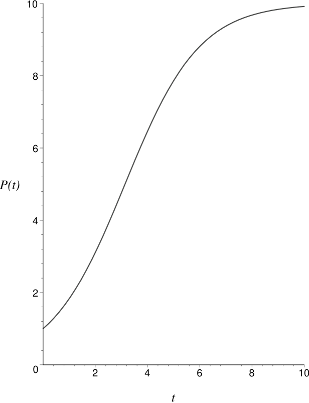
Figure 1. Logistic Curve with $M=10$, $P_{0}=1$, $k=0.7$

3. Approach Via Exponential Decay

Suppose instead of counting individuals, we count niches, viewing $M$ as the maximum number of niches the ecosystem can support, and $P$ as the number of niches currently occupied. Dimensional analysis suggests that instead of studying $P$, we consider

$$R=\frac{M-P}{P},$$ (3.1)

the dimensionless ratio of available or vacant niches to niches currently occupied. From (2.2), it readily follows that

$$\frac{1}{R}\frac{dR}{dt}=-k\qquad\Longrightarrow\qquad R(t)=R_{0}e^{-kt},$$ (3.2)

where $R_{0}$ is as in (2.3). Expressing (3.2) in terms of $P$, one arrives again at the solution (2.3).

For the instructor who would like to discuss logistic growth but would prefer to bypass separable differential equations and partial fractions, it may be desirable to “cut to the chase” by introducing the logistic model via (3.1) and (3.2) rather than via (2.2). In other words, although the fact that $R$ satisfies the differential equation (3.2) follows from its definition (3.1) and the logistic differential equation (2.2), one could equally well dispense with (2.2) and make (3.2) an assumption of the model, thereby proceeding more quickly to the solution. Of course, there are pedagogical advantages to either approach. One aspect the approach via (3.1) and (3.2) we are proposing has in its favour is that logistic growth can be introduced in the standard section on exponential growth and decay, with no loss in continuity and without any additional background.

That $R$ decreases at a rate proportional to itself, i.e. satisfies the differential equation (3.2), is intuitively plausible. Initially we think of $P$ being much smaller than $M$, so that $R$ is much larger than $1$ and many niches are available relative to the number currently occupied (a high niche vacancy rate). We should expect any species to take advantage of such a hospitable climate for reproduction, and hence initially, $R$ should decrease rapidly as $P$ increases. However, as the number of vacancies decreases, ($P$ gets close to $M$, $R$ gets close to zero) there are relatively few available niches remaining. In such an inhospitable climate, we should expect reproduction and hence further growth to be difficult, and accordingly, $R$ should decrease much more slowly. These considerations should be sufficient to motivate the introduction of logistic growth via (3.1) and (3.2) to any calculus or differential equations class.

4. Removing the Disguise

From the viewpoint of an individual of the species attempting to reproduce, one should expect a qualitative change in the hospitality of the ecosystem near $R=1$, given the considerations of the previous paragraph. Motivated by these considerations, we refer to an ecosystem as being hospitable or inhospitable according to whether $R$ is greater or less than 1. From (3.2), the transition from hospitable to inhospitable occurs when

$$t=\tau_{0}:=\frac{1}{k}\log R_{0}=\frac{1}{k}\log\left(\frac{M-P_{0}}{P_{0}}\right),\qquad R=1,\qquad P=\tfrac{1}{2}M.$$ (4.1)

It is well-known that this is precisely the time at which $P$ is increasing most rapidly, as can be seen by completing the square in (2.2):

$$\frac{dP}{dt}=\frac{Mk}{4}-\frac{k}{M}\left(P-\frac{M}{2}\right)^{2}.$$

Because of the distinguished nature of the point $(\tau_{0},M/2)$ it seems more sensible to measure time from $\tau_{0}$ than from zero. Certainly $t=0$ is completely arbitrary from the viewpoint of the species, having more to do with whatever external forces (desire, opportunity, availability of funding etc.) conspired to allow the biologist or census taker to obtain an initial field count than any essential features of the system. Therefore, we consider

$$Q(\tau):=P(\tau_{0}+\tau)-\tfrac{1}{2}M,$$

where $\tau$ measures time from $\tau_{0}$ and hence may be positive or negative. From (2.3), we have

$$Q(\tau)=\frac{M}{1+R_{0}e^{-k(\tau_{0}+\tau)}}-\frac{M}{2}.$$

Since $R_{0}e^{-k\tau_{0}}=1$, this simplifies to

$$Q(\tau)=\frac{M}{1+e^{-k\tau}}-\frac{M}{2}=\frac{M}{2}\left(\frac{1-e^{-k\tau}}{1+e^{-k\tau}}\right)=\tfrac{1}{2}{M}\tanh\left(\tfrac{1}{2}{k\tau}\right),$$ (4.2)

or in other words,

$$P(t)=\tfrac{1}{2}{M}\left(1+\tanh\left(\tfrac{1}{2}k(t-\tau_{0})\right)\right),$$ (4.3)

where $\tau_{0}$ is given by (4.1). Thus, the mysterious “S-shaped” [3, 6, 8] logistic curve is nothing more than a translate of our old and familiar friend, the hyperbolic tangent.

5. Addendum

If $0\leq P_{0}\leq M$, then $\infty\geq R_{0}\geq 0$. The boundary cases $P_{0}=0$ and $P_{0}=M$ correspond to $R_{0}=\infty,P(t)\equiv 0$ and $R_{0}=0,P(t)\equiv M$, respectively. To complete the analysis of logistic growth, it is necessary to consider what happens when $P_{0}$ lies outside the closed interval $[0,M]$, i.e. $R_{0}<0$. The solution (2.3) is valid for such $R_{0}$, but (4.3) was predicated on the assumption $R_{0}>0$ in the definition of $\tau_{0}$. Putting $S_{0}=-R_{0}$, we have from (2.3) that

$$P(t)=\frac{M}{1-S_{0}e^{-kt}},\qquad S_{0}>0.$$

In this case, we define

$$\tau_{0}:=\frac{1}{k}\log S_{0}\qquad\mbox{so that}\qquad e^{k\tau_{0}}=S_{0}=\frac{P_{0}-M}{P_{0}}.$$ (5.1)

A calculation analogous to (4.2) reveals that

$$H(\tau):=P(\tau_{0}+\tau)-\tfrac{1}{2}M=\tfrac{1}{2}M\coth\left(\tfrac{1}{2}k\tau\right),$$

or

$$P(t)=\tfrac{1}{2}M\left(1+\coth\left(\tfrac{1}{2}k(t-\tau_{0})\right)\right),$$ (5.2)

where now $\tau_{0}$ is given by (5.1).

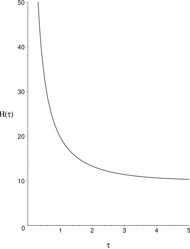
Figure 2. Logistic Curve with $M=10$, $P_{0}=30$, $k=0.7$

If $P_{0}>M$, then $-1\leq R_{0}<0$, $0<S_{0}=-R_{0}\leq 1$, and $-\infty<\tau_{0}\leq 0$. Therefore, for $t\geq 0$ we are on the upper arch of the hyperbolic cotangent, with population decreasing exponentially to $M$ as $t\to\infty$ (fig. 2). In the less biologically meaningful case $P_{0}<0$, we have $-1\geq R_{0}>-\infty$, $1\leq S_{0}=-R_{0}<\infty$ and $0\leq\tau_{0}<\infty$. As $t$ increases from zero to $\tau_{0}$, the rightmost portion of the lower arch of the hyperbolic cotangent is traversed, sending the population to minus infinity. The asymptote is then crossed and we skip over to the upper arch, the population reverting to its behaviour in the previous case.

References

- [1] W. Boyce and R. DiPrima, Elementary Differential Equations (5th ed.), John Wiley & Sons, New York, 1992, p. 54.
- [2] J. Callahan et al. Calculus in Context, W. H. Freeman and Company, New York, 1995, p. 161.
- [3] D. Hughes-Hallett et al. Calculus, John Wiley & Sons, New York, 1994, p. 532.
- [4] D. Powers, Elementary Differential Equations with Boundary Value Problems, Prindle, Weber & Schmidt, Boston, 1985, p. 21.
- [5] E. Rainville and P. Bedient, Elementary Differential Equations (7th ed.), Macmillan Publishing Company, New York, 1989, p. 55.
- [6] M. Spiegel, Applied Differential Equations (3rd ed.), Prentice-Hall, Inc., Englewood Cliffs, New Jersey, 1981, p. 155.
- [7] J. Stewart, Calculus Concepts and Contexts, Brooks/Cole, Boston, 1998, p. 505.
- [8] G. Strang, Calculus, Wellesley-Cambridge Press, Wellesley MA, 1991, p. 262.
- [9] K. Stroyan, Calculus: the Language of Change (2nd ed.), Academic Press, San Diego, 1998, p. 425.
- [10] R. Williamson, Introduction to Differential Equations and Dynamical Systems, McGraw-Hill, New York, 1997, p. 91.
- [11] D. Zill with W. Wright, Differential Equations with Computer Lab Experiments, PWS Publishing Company, Boston, 1995, p. 60.