Interfaces and the edge percolation map of random directed networks

Abstract

The traditional node percolation map of directed networks is reanalyzed in terms of edges. In the percolated phase, edges can mainly organize into five distinct giant connected components, interfaces bridging the communication of nodes in the strongly connected component and those in the in- and out-components. Formal equations for the relative sizes in number of edges of these giant structures are derived for arbitrary joint degree distributions in the presence of local and two-point correlations. The uncorrelated null model is fully solved analytically and compared against simulations, finding an excellent agreement between the theoretical predictions and the edge percolation map of synthetically generated networks with exponential or scale-free in-degree distribution and exponential out-degree distribution. Interfaces, and their internal organization giving place from “hairy ball” percolation landscapes to bottleneck straits, could bring new light to the discussion of how structure is interwoven with functionality, in particular in flow networks.

I Introduction

The theory of percolation applied to random networks Dorogovtsev et al. (2007) has proven to be one of the most notorious advances in complex networks science Albert and Barabási (2002); Dorogovtsev and Mendes (2003); Newman (2003a). Its importance goes beyond the production in the short term of theoretical results, which are general and relevant to systems in many different fields. The implication are far-reaching. On one hand, a number of different problems have a direct interpretation in terms of percolation or can be mapped to it, such as the study of resilience or vulnerability in front of random failures Cohen et al. (2000) or SIR epidemic spreading models Grassberger (1983); Sander et al. (2002, 2003); Newman (2002a); Kenah and Robins (2007); Miller (2007). On the other hand, the emergent percolation landscape can strongly affect properties such as fluency or navigability in self-organized systems. Hence, the conformation of connectivity structures in the percolated phase should ensure efficient communication at the global level so that different parts of the system–individuals, modules, or substructures- are able to interact for the whole to organize and develop functionality.

In the case of undirected networks, where elements are linked by channels operating in both directions, the basic percolation discussion was centered around the appearance of a macroscopic portion of connected nodes that are linked through undirected paths and so can communicate among them. The critical point for the appearance of this giant component and its relative size in number of nodes and edges was determined Molloy and Reed (1995, 1998); Cohen et al. (2000); Newman et al. (2001); Callaway et al. (2000), also in the presence of specific structural attributes Newman (2002b, 2003b); Vázquez and Moreno (2003); Dorogovtsev et al. (2001a); Krapivsky and Derrida (2004); Schwartz et al. (2002). In its turn, the standard picture in directed graphs Newman et al. (2001); Callaway et al. (2000); Dorogovtsev et al. (2001a, b); Boguñá and Ángeles Serrano (2005); Serrano and Boguñá (2006a, b) establishes that this giant connected component may become much more complex and internally organized in three main giant structures, the in-component, the out-component, and the strongly connected component, as well as other secondary aggregates such as tubes or tendrils. This conformation, sometimes represented as a bow-tie diagram Broder et al. (2000), denotes a potential global flow -of matter, energy, information…- organized around a core which usually processes input into output.

In this work, we will see that the percolation landscape, the aggregate of macroscopic connectivity structures in the percolated phase above the critical point, is further shaped when edges, the 0-level primary building blocks of networks along with nodes, are taken as starring elements. Five distinct components are found to be relevant in the edge percolation map of directed networks, the traditional strongly connected and the in and out node components, and two newly identified interfaces bridging the communication between them. In Sec. II, we define the relevant components and present analytical computations based on the generating function formalism and the usual locally treelike assumption for their relative size in number of edges in purely directed random networks that can present local and two-point correlations. In Sec. III, the formal equations for the most general situation will be reformulated for the prototypical null model of uncorrelated networks. The corresponding analytical results will be compared to simulations for networks with exponential in and out degree distributions and to numerical solutions associated to networks with scale-free in-degree and exponential out-degree distributions. A discussion of the implications coming out of this description will be provided in Sec. IV, where the concept of interface will be further examined along indications of the potential relevance of its internal structure, that could organize to produce from “hairy ball” percolation landscapes to bottleneck straits. We end by summarizing and giving some final remarks in Sec. V.

II Edge components in directed networks

In the traditional node percolation map of directed networks the core structure is the giant strongly connected component (GSCC), where all vertices within can reach each other by a directed path. When present, it serves as a connector of the giant in-component (GIN), composed by all vertices that can reach the GSCC but cannot be reached from it following directed paths, to the giant out-component (GOUT), made of all vertices that are reachable from the GSCC but cannot reach it following directed paths.

From the point of view of edges, the GIN and the GOUT unfold into two structures each, the edge in-component (ICE) and the in interface (ITF), and the edge out-component (OCE) and the out interface (OTF) respectively, so that five giant components should indeed be distinguished. This increase in the number of relevant structures is a consequence of the fact that nodes are point objects and they belong to just one of the three node components, whereas edges can be considered as extended objects in the sense that they could belong simultaneously to two different node components, having for instance one end in the GIN or GOUT and the other in the GSCC. This fact points to the necessity of defining new classes for edges. We will not take into account aggregates such as tendrils or tubes, so that edges will be classified into five different categories depending on the affiliation of the nodes they are joining. Let us recall that, in the node percolation map, the out- and in-components of individual vertices are defined as the number of vertices (plus itself), $s_{i}$, that are reachable from a given vertex and the number of vertices (plus itself), $s_{o}$, that can reach that vertex, respectively. The GSCC can be thus thought of as the set of vertices with infinite in- and out-components simultaneously, and the GOUT and GIN as the set of vertices with infinite in-component and infinite out-component respectively, excluding the GSCC. Taking this into consideration, we give the following definitions for the different principal components of the edge percolation map of random directed networks:

• The edge in-component, ICE, is the set of edges joining source and destination nodes with finite in-component and infinite out-component. These edges are connecting nodes within the GIN.

• The in-interface, ITF, is the set of edges joining source nodes with finite in-component and infinite out-component and destination nodes with infinite in- and out-components. These edges are bridging the ICE and the SCE (see below) by connecting nodes in the GIN to nodes in the SCC.

• The edge strongly connected component, SCE, is the set of edges joining source and destination nodes with infinite in- and out-components. These edges are connecting nodes within the SCC.

• The out-interface, OTF, is the set of edges joining source nodes with infinite in- and out-components and destination nodes with infinite in-component and finite out-component. These edges are bridging the SCE and the OCE by connecting nodes in the SCC to nodes in the GOUT.

• The edge out-component, OCE, is the set of edges joining source and destination nodes with infinite in-component and finite out-component. These edges are connecting nodes within the GOUT.

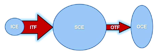
Figure 1: (color online). Schematic representation of the main giant components in the edge percolation map. As illustrated in the sketch, the different components can be heterogeneous in their sizes.

The critical point for the simultaneous appearance of the three giant node components -as well as other secondary structures such as tubes or tendrils- trivially marks also the emergence of the five giant edge components. In the most general case, the condition $\lambda_{m}>1$ characterizes the percolated phase, where $\lambda_{m}$ stands for the maximum eigenvalue of a characteristic matrix. In the case of purely directed random networks, where the main attribute of each node is its degree ${\bf k}\equiv(k_{i},k_{o})$ determined by its incoming and outgoing number of connections $k_{i}$ and $k_{o}$, the characteristic matrix in the presence of two-point correlations was found to be $C_{{\bf k}{\bf k^{\prime}}}^{o}$ (or $C_{{\bf k}{\bf k^{\prime}}}^{i}$ with the same results) Boguñá and Ángeles Serrano (2005),

$$\begin{array}[]{rrr}C_{{\bf k}{\bf k^{\prime}}}^{o}&=&k^{\prime}_{o}P_{o}({\bf k^{\prime}}|{\bf k})\\[8.5359pt] C_{{\bf k}{\bf k^{\prime}}}^{i}&=&k^{\prime}_{i}P_{i}({\bf k^{\prime}}|{\bf k}),\end{array}$$ (1)

where the transition probabilities $P_{i}({\bf k^{\prime}}|{\bf k})$ and $P_{o}({\bf k^{\prime}}|{\bf k})$ measure the likelihood to reach a vertex of degree ${\bf k^{\prime}}$ leaving from a vertex of degree ${\bf k}$ using an incoming and an outgoing edge, respectively. If the degrees of connected vertices are statistically uncorrelated, this condition reduces to the first-born Newman et al. (2001)

$$\sum_{k_{i},k_{o}}k_{o}(k_{i}-1)P(k_{i},k_{o})>0,$$ (2)

where $P(k_{i},k_{o})\equiv P({\bf k})$ is the joint degree distribution of in- and out-degrees, that could encode local correlations.

II.1 Analytical computation of edge components size in purely directed networks

In order to compute the sizes of the different giant components in number of edges, the already traditional approach used in previous developments is also appropriate with necessary adjustments. The mathematical methodology is based on the generating function formalism while the physical methodology explores the network with branching processes which expand under the locally treelike assumption Newman et al. (2001); Dorogovtsev et al. (2001b); Boguñá and Ángeles Serrano (2005). Maximally random purely directed networks with local and two-point correlations will be considered. This implies that the relevant information about the topology of the network is encoded in the joint degree distribution $P({\bf k},{\bf k^{\prime}})$, where ${\bf k}$ is the degree of the source node and k’ the degree of the destination node, or, equivalently, in the degree distribution $P({\bf k})$ along with the transition probabilities $P_{i}({\bf k^{\prime}}|{\bf k})$ and $P_{o}({\bf k^{\prime}}|{\bf k})$. These are related through the following degree detailed balance condition Boguñá and Pastor-Satorras (2002); Boguñá and Ángeles Serrano (2005)

$$k_{o}P({\bf k})P_{o}({\bf k^{\prime}}|{\bf k})=k^{\prime}_{i}P({\bf k^{\prime}})P_{i}({\bf k}|{\bf k^{\prime}}),$$ (3)

which is fulfilled whenever any edge leaving a vertex points to another or, in other words, whenever the network is closed and does not present dangling edge ends. Although the condition is satisfied for the whole graph, the three node components -GIN, GSCC, and GOUT- do not fulfill the detailed balance condition separately. If one restricts to consider the nodes within the boundaries of each component along all their connections, dangling ends can be found. The interfaces are just the sets of edges that prevent the node components from fulfilling the detailed balance condition separately.

Apart from the distributions above, the calculations also rely on the edge joint distribution $G(s_{i},s_{o};s^{\prime}_{i},s^{\prime}_{o})$ associated to directed edges joining source and destination vertices. It measures the simultaneous occurrence of finite sizes for the different single node components associated to the connected vertices. More specifically, it measures the number of vertices (plus itself), $s_{o}$, that are reachable from the source vertex and the number of vertices (plus itself), $s_{i}$, that can reach the source vertex, simultaneously to the number of vertices (plus itself), $s^{\prime}_{o}$, that are reachable from the destination vertex and the number of vertices (plus itself), $s^{\prime}_{i}$, that can reach the destination vertex. Notice that if computations are done for node components, the relevant distribution is $G(s_{i},s_{o})$ and refers to just one node. According to the definitions above, and as a function of the edge joint distribution, the relative sizes of the different giant edge components can be formally written as

$$g_{ice} = \sum_{s_{i}}\sum_{s^{\prime}_{i}}G(s_{i},s_{o}=\infty;s^{\prime}_{i},s^{\prime}_{o}=\infty)$$

$$g_{oce} = \sum_{s_{o}}\sum_{s^{\prime}_{o}}G(s_{i}=\infty,s_{o};s^{\prime}_{i}=\infty,s^{\prime}_{o})$$

$$g_{itf} = \sum_{s_{i}}G(s_{i},s_{o}=\infty;s^{\prime}_{i}=\infty,s^{\prime}_{o}=\infty)$$

$$g_{otf} = \sum_{s^{\prime}_{o}}G(s_{i}=\infty,s_{o}=\infty;s^{\prime}_{i}=\infty,s^{\prime}_{o})$$

$$g_{sce} = G(s_{i}=\infty,s_{o}=\infty;s^{\prime}_{i}=\infty,s^{\prime}_{o}=\infty),$$ (4)

where we have made use of the fact that if the destination node has an infinite out-component so it has the source node and, analogously, if the in-component of the source node is infinite so will be the in-component of the destination node. These functions can be computed from the marginal distributions associated to $G(s_{i},s_{o};s^{\prime}_{i},s^{\prime}_{o})$, which preserve just some of the four variables. Their dependence on a given variable $s_{i/o}$ indicates that the corresponding in or out-component of the source or destination vertex (destination vertex with prima) is finite with size $s_{i/o}$ regardless of the size of the rest of the involved single node components. For instance, the function $G(s_{i},;s^{\prime}_{i},)$ measures the probability of an edge connecting a source node with finite in-component of size $s_{i}$ to a destination node with finite in-component of size $s^{\prime}_{i}$, regardless of the sizes of the out-components of connected nodes, that could be finite or infinite (notice that for ease of notation we just left blank the spaces corresponding to the marginalized variables). In terms of these marginal probabilities, the relative sizes of the main components are:

$$g_{ice} = \sum_{s_{i},s^{\prime}_{i}}G(s_{i},;s^{\prime}_{i},)-\sum_{s_{i},s^{\prime}_{i},s^{\prime}_{o}}G(s_{i},;s^{\prime}_{i},s^{\prime}_{o})$$

$$g_{oce} = \sum_{s_{o},s^{\prime}_{o}}G(,s_{o};,s^{\prime}_{o})-\sum_{s_{i},s_{o},s^{\prime}_{o}}G(s_{i},s_{o};,s^{\prime}_{o})$$

$$g_{itf} = \sum_{s_{i}}G(s_{i},;,)-\sum_{s_{i},s^{\prime}_{i}}G(s_{i},;s^{\prime}_{i},)-$$

$$\sum_{s_{i},s^{\prime}_{o}}G(s_{i},;,s^{\prime}_{o})+\sum_{s_{i},s^{\prime}_{i},s^{\prime}_{o}}G(s_{i},;s^{\prime}_{i},s^{\prime}_{o})$$

$$g_{otf} = \sum_{s^{\prime}_{o}}G(,;,s^{\prime}_{o})-\sum_{s_{o},s^{\prime}_{o}}G(,s_{o};,s^{\prime}_{o})-$$

$$\sum_{s_{i},s^{\prime}_{out}}G(s_{i},;,s^{\prime}_{o})+\sum_{s_{i},s_{o},s^{\prime}_{o}}G(s_{i},s_{o};,s^{\prime}_{o})$$

$$g_{sce} = 1-\sum_{s_{i}}G(s_{i},;,)-\sum_{s^{\prime}_{o}}G(,;,s^{\prime}_{o})+$$ (5)

$$\sum_{s_{i},s^{\prime}_{o}}G(s_{i},;,s^{\prime}_{o}).$$

These marginal probabilities depend on the degrees of the nodes at the ends of the edge under consideration. Edges connecting nodes in the same degree classes will be considered statistically equivalent, so that these functions should be rewritten over joint degree classes. For instance,

$$G(s_{i},;s_{i},s^{\prime}_{o})=\sum_{{\bf k},{\bf k^{\prime}}}P({\bf k},{\bf k^{\prime}})G(s_{i},;s_{i},s^{\prime}_{o}|{\bf k},{\bf k^{\prime}}),$$ (6)

and analogously for the rest. To calculate these conditional probabilities we have to introduce at this point the probability functions $g_{o}(s|{\bf k})$ and $g_{i}(s|{\bf k})$, which represent the distributions of the number of reachable vertices from a vertex, given that we have arrived to it from another source vertex of degree ${\bf k}$ following one of its outgoing or incoming edges, respectively. These functions are exactly the same as those already introduced in previous works for the computation of the sizes of the GIN, GOUT and GSCC. The marginal conditional probabilities can then be expressed as functions of these single-node probabilities, that in its turn obey closed equations obtained from an iterative procedure which applies the techniques of random branching processes under the locally treelike assumption. This hypothesis is correct if the length of cycles present in the network is of the order of its diameter, so that the sizes of single node components can be exposed by subsequent jumps from neighbors to neighbors of neighbors without returning to already visited ones (the presence of lower order loops would induce overcounting). In this way, the problem can be formally solved in the general correlated case.

As a way of example, it will suffice here to provide the expression of one of the marginal conditional distributions as a function of $g_{o}(s|{\bf k})$ and $g_{i}(s|{\bf k})$ to illustrate the derivation. Assuming the locally treelike condition, one of the two relevant marginal conditional probabilities in the computation of the ICE can be written as

$$G(s_{i},;s^{\prime}_{i},s^{\prime}_{o}|{\bf k},{\bf k^{\prime}}) = \sum_{s_{1}^{i}\cdots s_{k_{i}}^{i}}g_{i}(s_{1}^{i}|{\bf k})\cdots g_{i}(s_{k_{i}}^{i}|{\bf k})\delta_{s_{1}^{i}+\cdots+s_{k_{i}}^{i}+1,s_{i}}$$ (7)

$$\times \sum_{s_{1}^{{}^{\prime}i}\cdots s_{k^{\prime}_{i}-1}^{{}^{\prime}i}}g_{i}(s_{1}^{{}^{\prime}i}|{\bf k^{\prime}})\cdots g_{i}(s_{k^{\prime}_{i}-1}^{{}^{\prime}i}|{\bf k^{\prime}})\delta_{s_{i}+s_{1}^{{}^{\prime}i}+\cdots+s_{k_{i}-1}^{{}^{\prime}i}+1,s^{\prime}_{i}}$$

$$\times \sum_{s_{1}^{{}^{\prime}o}\cdots s_{k^{\prime}_{o}}^{{}^{\prime}o}}g_{o}(s_{1}^{{}^{\prime}o}|{\bf k^{\prime}})\cdots g_{o}(s_{k^{\prime}_{o}}^{{}^{\prime}o}|{\bf k^{\prime}})\delta_{s_{1}^{{}^{\prime}o}+\cdots+s_{k_{o}}^{{}^{\prime}o}+1,s^{\prime}_{o}}.$$

This expression for the joint multi-component conditional size distribution $G(s_{i};s^{\prime}_{i},s^{\prime}_{o}|{\bf k},{\bf k^{\prime}})$ needs three simultaneous computations: the number of vertices that can reach the source node, the number of vertices that can reach the destination node, and the number of nodes that the destination node can reach itself. The procedure starts from an edge linking nodes of degrees ${\bf k}$ and ${\bf k^{\prime}}$ and splits the sets $s_{i}$, $s^{\prime}_{i}$ and $s^{\prime}_{o}$ into the different contributions associated to the corresponding neighbors. For instance, the number of edges that bring to the degree-${\bf k}$ source node, $s_{i}$, can be computed as the sum of the different contributions that can reach each of its $k_{i}$ incoming neighbors, $s^{i}_{1}+\cdots+s^{i}_{k_{i}}$. This corresponds to the first set of summations of the three that appear in Eq. (7). Independent equations for the functions $g_{i}$ and $g_{o}$ can be found by expanding iteratively this procedure:

$$g_{i}(s|{\bf k}) = \sum_{\bf k^{\prime}}P_{i}({\bf k^{\prime}}|{\bf k})g_{i}(s_{1}|{\bf k^{\prime}})\cdots g_{i}(s_{k^{\prime}_{i}}|{\bf k^{\prime}})\delta_{S_{k^{\prime}_{i}},s}$$

$$g_{o}(s|{\bf k}) = \sum_{\bf k^{\prime}}P_{o}({\bf k^{\prime}}|{\bf k})g_{o}(s_{1}|{\bf k^{\prime}})\cdots g_{o}(s_{k^{\prime}_{o}}|{\bf k^{\prime}})\delta_{S_{k^{\prime}_{o}},s},$$ (8)

where $S_{k^{\prime}_{i}}=s_{1}+\cdots+s_{k^{\prime}_{i}}+1$ and $S_{k^{\prime}_{o}}=s_{1}+\cdots+s_{k^{\prime}_{o}}+1$. These equations become tractable using the generating function formalism. In mathematical terms, generating functions are obtained by applying the transformation $\hat{f}(z)\equiv\sum_{s}f(s)z^{s}$, so that functions are brought to the discrete Laplace space. Once transformed for the variables $s$, Eqs. (8) become closed for $\hat{g}_{i}$ and $\hat{g}_{o}$,

$$\hat{g}_{i}(z|{\bf k}) = z\sum_{\bf k^{\prime}}P_{i}({\bf k^{\prime}}|{\bf k})\hat{g}_{i}(z|{\bf k^{\prime}})^{k^{\prime}_{i}}$$

$$\hat{g}_{o}(z|{\bf k}) = z\sum_{\bf k^{\prime}}P_{o}({\bf k^{\prime}}|{\bf k})\hat{g}_{o}(z|{\bf k^{\prime}})^{k^{\prime}_{o}}.$$ (9)

All summations over finite sizes of the joint conditional size distributions correspond to their generating functions evaluated at $z=1$. Eventually, those depend on $\hat{g}_{i}(1|{\bf k})$ and $\hat{g}_{i}(1|{\bf k})$:

$$\hat{G}(1,;1,1) = \sum_{{\bf k},{\bf k^{\prime}}}P({\bf k},{\bf k^{\prime}})\hat{g}_{i}(1|{\bf k})^{k_{i}}\hat{g}_{i}(1|{\bf k^{\prime}})^{k^{\prime}_{i}-1}\hat{g}_{o}(1|{\bf k^{\prime}})^{k^{\prime}_{o}}$$

$$\hat{G}(1,1;,1) = \sum_{{\bf k},{\bf k^{\prime}}}P({\bf k},{\bf k^{\prime}})\hat{g}_{i}(1|{\bf k})^{k_{i}}\hat{g}_{o}(1|{\bf k})^{k_{o}-1}\hat{g}_{o}(1|{\bf k^{\prime}})^{k^{\prime}_{o}}$$

$$\hat{G}(,1;,1) = \sum_{{\bf k},{\bf k^{\prime}}}P({\bf k},{\bf k^{\prime}})\hat{g}_{o}(1|{\bf k})^{k_{o}-1}\hat{g}_{o}(1|{\bf k^{\prime}})^{k^{\prime}_{o}}$$

$$\hat{G}(1,;1,) = \sum_{{\bf k},{\bf k^{\prime}}}P({\bf k},{\bf k^{\prime}})\hat{g}_{i}(1|{\bf k})^{k_{i}}\hat{g}_{i}(1|{\bf k^{\prime}})^{k^{\prime}_{i}-1}$$

$$\hat{G}(1,;,1) = \sum_{{\bf k},{\bf k^{\prime}}}P({\bf k},{\bf k^{\prime}})\hat{g}_{i}(1|{\bf k})^{k_{i}}\hat{g}_{o}(1|{\bf k^{\prime}})^{k^{\prime}_{o}}$$

$$\hat{G}(,;,1) = \sum_{{\bf k},{\bf k^{\prime}}}P({\bf k},{\bf k^{\prime}})\hat{g}_{o}(1|{\bf k^{\prime}})^{k^{\prime}_{o}}$$

$$\hat{G}(1,;,) = \sum_{{\bf k},{\bf k^{\prime}}}P({\bf k},{\bf k^{\prime}})\hat{g}_{i}(1|{\bf k})^{k_{i}}.$$ (10)

These expressions will allow us to compute easily the relative sizes of the different components:

$$g_{ice} = \hat{G}(1,;1,)-\hat{G}(1,;1,1)$$

$$g_{oce} = \hat{G}(,1;,1)-\hat{G}(1,1;,1)$$

$$g_{itf} = \hat{G}(1,;,)-\hat{G}(1,;1,)-\hat{G}(1,;,1)+\hat{G}(1,;1,1)$$

$$g_{otf} = \hat{G}(,;,1)-\hat{G}(,1;,1)-\hat{G}(1,;,1)+\hat{G}(1,1;,1)$$

$$g_{sce} = 1-\hat{G}(1,;,)-\hat{G}(,;,1)+\hat{G}(1,;,1).$$ (11)

Notice that the sizes of the interfaces can also be written as

$$g_{itf} = \hat{G}(1,;,)-\hat{G}(1,;,1)-g_{ice}$$

$$g_{otf} = \hat{G}(,;,1)-\hat{G}(1,;,1)-g_{oce}.$$

The set of Eqs. (9)-(10)-(11) determines completely the relative sizes in number of edges of the main giant components of the edge percolation map of two-point correlated purely directed networks.

III Uncorrelated purely directed networks

The formal solution given in the previous section becomes simpler for the classical null model of uncorrelated networks. This will allow us to perform further analytical computations that will be checked against simulation results in order to contrast the accuracy of the theory.

The absence of two-point correlations make possible to factorize the joint degree distribution, and the conditional degree distributions also simplify:

$$P({\bf k},{\bf k^{\prime}})=\frac{k^{\prime}_{i}k_{o}P({\bf k})P({\bf k^{\prime}})}{\langle k_{i}\rangle^{2}}$$ (13)

and

$$P_{o}({\bf k^{\prime}}|{\bf k})=\frac{k^{\prime}_{i}P({\bf k^{\prime}})}{\langle k_{i}\rangle}\mbox{ , }P_{i}({\bf k^{\prime}}|{\bf k})=\frac{k^{\prime}_{o}P({\bf k^{\prime}})}{\langle k_{i}\rangle}.$$ (14)

In this situation, Eqs. (9) evaluated in $z=1$ reduce to

$$\hat{g}_{i}(1|{\bf k}) \equiv \hat{g}_{i}(1)=\sum_{\bf k}\frac{k_{o}P({\bf k})}{\langle k_{i}\rangle}\hat{g}_{i}(1)^{k_{i}}$$

$$\hat{g}_{o}(1|{\bf k}) \equiv \hat{g}_{o}(1)=\sum_{\bf k}\frac{k_{i}P({\bf k})}{\langle k_{i}\rangle}\hat{g}_{o}(1)^{k_{o}},$$ (15)

so that the relative sizes in number of edges of the different components in the uncorrelated case just depend on the joint degree distribution $P({\bf k})$ and the single-node in and out generating functions $\hat{g}_{i}(1)$ and $\hat{g}_{o}(1)$, and can be written as

$$g_{ice} = \sum_{\bf k}\frac{k_{i}P({\bf k})}{\langle k_{i}\rangle}\hat{g}_{i}(1)^{k_{i}}(1-\hat{g}_{o}(1)^{k_{o}})$$

$$g_{oce} = \sum_{\bf k}\frac{k_{o}P({\bf k})}{\langle k_{i}\rangle}\hat{g}_{o}(1)^{k_{o}}(1-\hat{g}_{i}(1)^{k_{i}})$$

$$g_{itf} = \hat{g}_{i}(1)(1-\hat{g}_{o}(1))-g_{ice}$$

$$g_{otf} = \hat{g}_{o}(1)(1-\hat{g}_{i}(1))-g_{oce}$$

$$g_{sce} = (1-\hat{g}_{i}(1))(1-\hat{g}_{o}(1)).$$ (16)

If local correlations are also absent, the expressions above become even simpler

$$g_{ice} = (1-\hat{g}_{o}(1))\sum_{k_{i}}\frac{k_{i}\hat{g}_{i}(1)^{k_{i}}P(k_{i})}{\langle k_{i}\rangle}$$

$$g_{oce} = (1-\hat{g}_{i}(1))\sum_{k_{o}}\frac{k_{o}\hat{g}_{o}(1)^{k_{o}}P(k_{o})}{\langle k_{i}\rangle}$$

$$g_{itf} = (1-\hat{g}_{o}(1))\hat{g}_{i}(1)-g_{ice}$$

$$g_{otf} = (1-\hat{g}_{i}(1))\hat{g}_{o}(1)-g_{oce}$$

$$g_{sce} = (1-\hat{g}_{i}(1))(1-\hat{g}_{o}(1))$$ (17)

with

$$\hat{g}_{i}(1)=\sum_{k_{i}}P(k_{i})\hat{g}_{i}(1)^{k_{i}}$$

$$\hat{g}_{o}(1)=\sum_{k_{o}}P(k_{o})\hat{g}_{o}(1)^{k_{o}}.$$ (18)

III.1 Comparing against simulations

In order to ascertain the accuracy of the theory, we contrast the analytical results with those obtained from simulating uncorrelated purely directed networks with given joint degree distribution of the form $P({\bf k})=P(k_{i})P(k_{o})$. Uncorrelated networks are generated according to a slightly modified version of the Molloy-Reed prescription Molloy and Reed (1995, 1998) -which is based on the configuration model Bender and Canfield (1978); Bollobás (1980) and constructs maximally random networks with a given degree sequence- to produce directed connections controlling that $\sum_{i}k_{i}=\sum_{o}k_{o}$ and also taking care of avoiding multiple or self-connections.

III.1.1 Exponential in- and out-degree distributions

For the first case study, we chose $P(k_{i})$ and $P(k_{o})$ of the form

$$P(k)=\left\{\begin{array}[]{lr}P_{0}&k=0\\[14.22636pt] \displaystyle{\frac{(1-P_{0})^{2}}{\langle k\rangle}}\left[1-\frac{(1-P_{0})}{\langle k\rangle}\right]^{k-1}&k\geq 1\end{array}\right.,$$ (19)

so that a full analytical solution is available. The sizes of the giant components in the edge percolation map for this particular joint degree distribution just depend on the parameters $P_{0}^{i}$ and $P_{0}^{o}$ and the average degree $\langle k_{i}\rangle=\langle k_{o}\rangle$. Substituting Eqs. (19) into Eqs. (18), the solutions are found to be

$$\hat{g}_{i}(1)=\frac{P_{0}^{i}}{q^{i}}\mbox{ , }\hat{g}_{o}(1)=\frac{P_{0}^{o}}{q^{o}}\mbox{ , }q=1-\frac{1-P_{0}}{\langle k_{i}\rangle},$$ (20)

and the relative sizes

$$g_{ice} = \frac{\hat{g}_{i}(1)(1-\hat{g}_{o}(1))}{\langle k_{i}\rangle^{2}}$$

$$g_{oce} = \frac{\hat{g}_{o}(1)(1-\hat{g}_{i}(1))}{\langle k_{i}\rangle^{2}}$$

$$g_{itf} = \frac{\hat{g}_{i}(1)(1-\hat{g}_{o}(1))}{\langle k_{i}\rangle^{2}}(\langle k_{i}\rangle^{2}-1)$$

$$g_{otf} = \frac{\hat{g}_{o}(1)(1-\hat{g}_{i}(1))}{\langle k_{i}\rangle^{2}}(\langle k_{i}\rangle^{2}-1)$$

$$g_{sce} = (1-\hat{g}_{i}(1))(1-\hat{g}_{o}(1)).$$ (21)

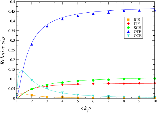
Figure 2: (color online). Relative sizes of the main giant components in the edge percolation map of networks with exponential in- and out-degree distributions as a function of the average degree. Simulation results (dots) correspond to 1-realization measures on synthetic networks with $N=10^{5}$ vertices, $P_{0}^{i}=0.4$, and $P_{0}^{o}=0.8$. Solid lines are the analytical solutions Eqs. (20)-(21).

We compared these results with direct measures of the edge components on a synthetic set of purely directed random networks with $N=10^{5}$. We fix the values $P_{0}^{i}=0.4$, $P_{0}^{o}=0.8$, and vary the average degree from $\langle k_{i}\rangle=1$ to $\langle k_{i}\rangle=10$. As Fig. 2 shows, the conformity of our formulas to the simulation results is excellent. Notice also that for this particular choice of the parameters $P_{0}^{i}$ and $P_{0}^{o}$, the out-interface, OCE, is by far the biggest edge component in the percolated phase for all values of the average degree above approximately $1.5$ , followed with a noticeable difference by the edge strongly connected component, SCE, and the in interface, ICE. In this example, the interfaces are much stronger than the edge in- and out-components, practically absent for high degrees. This edge percolation map is seen to be quite stable for most of the average degree range (see Sec. IV for further discussion).

III.1.2 Scale-free in-degree and exponential out-degree distributions

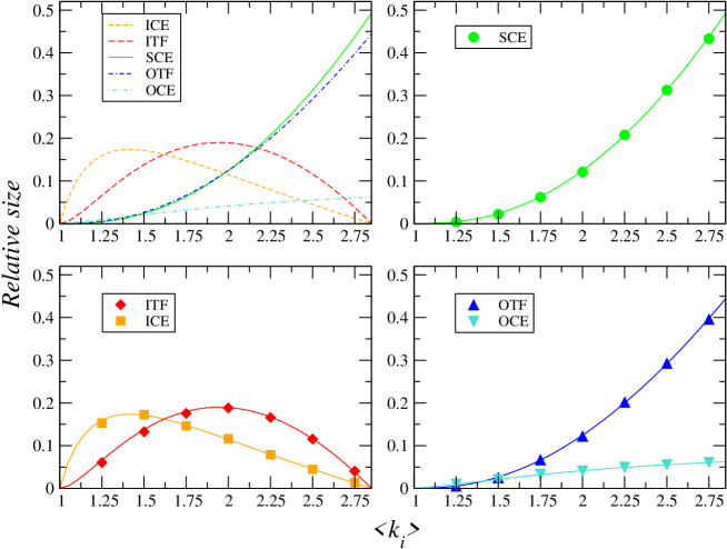
Figure 3: (color online). Relative sizes of the giant components in the edge percolation map of uncorrelated networks with scale-free in-degree distribution, $\gamma=2.2$, and exponential out-degree distribution, $P_{0}^{out}=0.4$, as a function of the average degree. Simulation results (dots) correspond to synthetic networks of size $N=5\cdot 10^{5}$ vertices, 3 realizations for the first two point and one realization for the rest. Solid lines correspond to the numerical solutions of Eqs. (17)-(18).

In some real networks, such as the WWW Serrano et al. (2007) for instance, the in-degree distribution exhibits a heavy-tailed form well approximated by a power-law behavior $P(k_{i})\sim k_{i}^{-\gamma}$, at the same time that a different functional dependence is faced in the case of the out-degree distribution $P(k_{o})$, which can present clear exponential cut-offs. In biology, transcriptional regulatory networks are characterized by the reflexive situation, in which an incoming degree distribution that decays faster than a power law can be observed along with a scale-free outgoing degree distribution Vázquez et al. (2004). It is then particularly interesting to see what happens for power law in- or out-degree distributions when combined to exponential out- or in-degree ones. In this example, the in-degree distribution is taken to follow a scale-free form of the type

$$P_{i}(k)=\left\{\begin{array}[]{lr}P_{0}&k=0\\[14.22636pt] \displaystyle{\frac{(1-P_{0})}{\zeta(\gamma)k^{\gamma}}}&k\geq 1\end{array}\right.,$$ (22)

where $\zeta(\gamma)$ is the Zeta Riemann function. The out-degree distribution is given again by Eq. (19). The set of Eqs. (18) is solved numerically and plugged into Eqs. (17) to get the relative sizes of the edge components and the results are compared to direct measures of the edge percolation map on a set of synthetically generated networks with $N=5\cdot 10^{5}$ nodes. We take $\gamma=2.2$, $P_{0}^{o}=0.4$ and vary the average degree $\langle k_{i}\rangle=\langle k_{o}\rangle$ until the maximum possible value is reached by adjusting $P_{0}^{i}$. This upper boundary in the average degree is due to the fact that, since $P_{0}^{i}=1-\langle k_{i}\rangle\zeta(\gamma)/\zeta(\gamma-1)$, values above the threshold impose a negative $P_{0}^{i}$ and are not realizable. The theoretical value for this threshold is $\zeta(\gamma-1)/\zeta(\gamma)$.

Once again, our predictions compare extremely well with the measures on the simulated networks, see Fig. 3. Interestingly, and in contrast to what was obtained in the previous example, the edge percolation map changes dramatically depending on the average degree. For small values –but big enough to ensure that the system is in the percolated phase, $\langle k_{i}\rangle>1$–, the edge in-component, ICE, and the in-interface, ITF, are predominant. However, the rest of edge components grow steadily with the average degree while those reach a maximum and then decay to eventually disappear at the average degree threshold, so that for high values of the average degree the edge strongly connected component, SCE, and the out-interface, OTF, dominate.

IV Interfaces

Interfaces arise as distinctive elements of the edge percolation map. From the analytical computations one sees that the interfaces are also giant components. Furthermore, their size could be much larger than that of the ICE and OCE, for instance as shown in Figs. 2 and 3. In the particular case of the completely uncorrelated networks with exponential in- and out-degree distributions given by Eq.(19), the relative sizes of the interfaces as compared to that of the pure components can be calculated analytically and found to be

$$\frac{g_{itf}}{g_{ice}}=\frac{g_{otf}}{g_{oce}}={\langle k_{i}\rangle}^{2}-1.$$ (23)

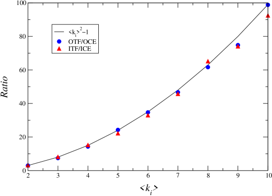
Figure 4: (color online). Ratio of the relative sizes of the giant interfaces to the edge in- and out-components as as a function of the average degree. Simulation results (dots) correspond to 1-realization networks of size $N=10^{5}$ vertices with $P_{0}^{i}=0.4$ and $P_{0}^{o}=0.8$. Solid line correspond to the analytical ratio Eq. (23).

The same relation is numerically seen to happen for the ratio between the out-interface and the edge out-component of the second case study where the in-degree distribution was scale-free and the out-degree distribution exponential. So, for exponential distributions the ratio of the relative sizes of the giant interfaces to the corresponding in- or out-component grows quadratically with the average degree. This result is very interesting because it suggests that, at least in this case, the traditional GIN and GOUT components of the node percolation map show a shallow architecture mainly formed by leaf edges emanating from or pointing to the SCC. As a consequence, and to give a mental image, the bow-tie structure of those networks rather becomes a “hairy ball”.

All this points to a rich second order fine structure that could play a central role in the investigation of how topology is related to functionality. In particular, and apart from the information contained in both the node and edge percolation maps, the internal structure of the interfaces, and more specifically the distinction of leaf edges from connectors, is fundamental in order to assess the efficiency of the global flow or the risks of bottleneck effects. Further discussion about the internal structure of interfaces and possible implications will be provided in a forthcoming work.

IV.1 Internal average degrees

Interfaces have a hybrid nature from the point of view of node components. In order to calculate internal average degrees, it is not clear whether they should be assigned to one node component or another. If one considers for instance the subset of nodes in the SCC with all their connections, internal or not, it is found that

$$\frac{\sum_{SCC}k_{i}}{E}=g_{sce}+g_{itf}\mbox{ , }\frac{\sum_{SCC}k_{o}}{E}=g_{sce}+g_{otf},$$ (24)

where $E$ is the total number of edges in the network. As a consequence, the detailed balance condition Eq. (3) will not be accomplished in general, $\sum_{SCC}k_{i}\neq\sum_{SCC}k_{o}$, except when both interfaces are of equal sizes. The same happens for the subsets of nodes in the GIN and the GOUT, where from the point of view of detailed balance there is an excess out- and in-degree respectively. The interfaces are precisely the responsible for these imbalances.

We explore once more as a null model that can be fully calculated analytically the completely uncorrelated network, with no local or degree-degree correlations. In this situation, the sizes of the main components in the node percolation map can be expressed as (see Refs. Newman (2002b); Dorogovtsev et al. (2001a); Boguñá and Ángeles Serrano (2005))

$$g_{scc} = 1-\hat{g}_{o}(1)-\hat{g}_{i}(1)+\hat{g}_{o}(1)\hat{g}_{i}(1)$$

$$g_{in} = 1-\hat{g}_{o}(1)-g_{scc}$$

$$g_{out} = 1-\hat{g}_{i}(1)-g_{scc},$$ (25)

where $\hat{g}_{i}(1)$ and $\hat{g}_{o}(1)$ are the solutions of Eq. (18), like for the edge percolation map. Comparing Eq. (25) and Eq. (17), it is found that the relative sizes in number of nodes of the GIN, GOUT, and SCC are the same as the relative sizes in number of edges of the ICE+ITF, OCE+OTF, and SCE respectively. In other words, the average degree of the whole network is preserved in the different components if the in- and out-interfaces are assigned to the in- and out-components respectively. This is in particular valid for the previous examples of uncorrelated networks with exponential or scale-free in-degree distribution and exponential out-degree distribution.

V Conclusions

We focus on edges instead of nodes to investigate analytically how they organize in the percolated phase of purely directed random networks. Interfaces of edges are found to bridge the main components of the node percolation map. The general case of local and degree-degree correlations is formally solved and the relative sizes of the five main giant edge components are characterized quantitatively. The results for uncorrelated networks are found to be in very good agreement with direct measures on synthetic networks, that could present very different edge percolation maps depending on the in- and out-degree distributions and the average degree.

The node percolation map is in this way complemented by the edge percolation map, forming a percolation landscape that gives a more detailed topological description of the structure of globally connected systems. The work should not stop here, since results in this paper seem to point out to the importance of the internal organization of the interfaces with latent implications at the level of functional properties. So, the analysis presented in this work uncovers a new aspect potentially relevant not only for the structure of directed networks but most importantly for their functionality. Generally, the SCC processes input into output so that interfaces become unavoidable bridges that could determine the effectiveness or the robustness of functional performance.

In this work, we have restricted to purely directed networks, a good approximation in many cases where flow or transport, when present in both directions, is asymmetric. Nevertheless, the same ideas can be extended to semi-directed networks, the most general and realistic ones. For those, analytical calculations could be a bit more intricate due to the non-trivial correlations associated to reciprocity.