WiFi Epidemiology: Can Your Neighbors’ Router Make Yours Sick?

¹Department of Physics, Indiana University, Bloomington, IN 47405, USA

²School of Informatics, Indiana University, Bloomington, IN 47406, USA

³Complex Networks Lagrange Laboratory, Institute for Scientific Interchange (ISI), Torino 10133, Italy

^∗e-mail: samyers@indiana.edu
In densely populated urban areas WiFi routers form a tightly interconnected proximity network that can be exploited as a substrate for the spreading of malware able to launch massive fraudulent attack and affect entire urban areas WiFi networks. In this paper we consider several scenarios for the deployment of malware that spreads solely over the wireless channel of major urban areas in the US. We develop an epidemiological model that takes into consideration prevalent security flaws on these routers. The spread of such a contagion is simulated on real-world data for geo-referenced wireless routers. We uncover a major weakness of WiFi networks in that most of the simulated scenarios show tens of thousands of routers infected in as little time as two weeks, with the majority of the infections occurring in the first 24 to 48 hours. We indicate possible containment and prevention measure to limit the eventual harm of such an attack.

Correspondence and requests for material should be addressed to S.M. (samyers@indiana.edu) or A.V. (alexv@indiana.edu).

The use of WiFi routers is becoming close to mainstream in the US and Europe, with 8.4% and 7.9% of all such respective households having deployed such routers by 2006 ¹, and a WiFi market expected to grow quickly in the next few years as more new digital home devices are being shipped with WiFi technology. In 2006 alone 200 million WiFi chipsets were shipped worldwide, representing nearly half of the 500 million cumulative total ². As the WiFi deployment becomes more and more pervasive, the larger is the risk that massive attacks exploiting the WiFi security weaknesses could affect large numbers of users.

Recent years have witnessed a change in the designers behind a malware attack and in their motivations, corresponding to the ever increasing sophistication needed to bypass newly developed security technologies. Malware creators have shifted from programmer enthusiasts attempting to get peer credit from the “hacker” community, to organized crime engaging in fraud and money laundering through different forms of online crime. In this context WiFi routers represent valuable targets when compared to the PC’s that malware traditionally infect, as they have several differing properties representing strong incentives for the attacks. They are the perfect platform to launch a number of fraudulent attacks ^{3, 4, 5, 6} that previous security technologies have reasonably assumed were unlikely ⁷. Unlike PCs, they tend to be always on and connected to the Internet, and currently there is no software aimed at specifically detecting or preventing their infection. Further, as routers need to be within relatively close proximity to each other to communicate wirelessly, an attack can now take advantage of the increasing density of WiFi routers in urban areas that creates large geographical networks where the malware can propagate undisturbed. Indeed, many WiFi security threats have been downplayed based on the belief that the physical proximity needed for the potential attack to occur would represent an obstacle for attackers. The presence nowadays of large ad-hoc networks of routers make these vulnerabilities considerably more risky than previously believed.

Here we assess for the first time the vulnerability of WiFi networks of different US cities by simulating the wireless propagation of malware, a malicious worm spreading directly from wireless router to wireless router. We construct an epidemiological model that takes into account several widely known and prevalent weaknesses in commonly deployed WiFi routers’ security ^{3, 8}, (e.g., default and poor password selection and cracks in the WEP cryptographic protocol ⁹). The WiFi proximity networks over which the attack is simulated are obtained from real-world geographic location data for wireless routers. The infection scenarios obtained for a variety of US urban areas are troublesome in that the infection of a small number of routers in most of these cities can lead to the infection of tens of thousands of routers in a week, with most of the infection occurring in the first 24 hours. We address quantitatively the behavior of the spreading process and we provide specific suggestions to minimize the WiFi network weakness and mitigate an eventual attack.

Results and Discussion

WiFi networks. WiFi routers, even if generally deployed without a global organizing principle, define a self-organized proximity communication network. Indeed, any two routers which are in the range of each other’s WiFi signal can exchange information and may define an ad-hoc communication network. These networks belong to the class of spatial or geometric networks in that nodes are embedded in a metric space and the interaction between two nodes strongly depends on the range of their spatial interaction ^{10, 11, 12, 13}.

In this perspective, one might wonder if the actual deployment of WiFi routers is sufficient at the moment to generate large connected networks spanning sizeable geographic areas. This problem, equivalent to the percolation of giant connected component in graph theory^{14, 15}, is however constrained by the urban area’s topology and demographic distribution dictating the geographical locations of WiFi routers. Here we consider WiFi networks as obtained from the public worldwide database of the Wireless Geographic Logging Engine (WiGLE) website ¹⁶. The database collects data on the worldwide geographic location of wireless routers and counts more than $10$ million unique networks on just under 600 million observations ¹⁷, providing good coverage of the wireless networks in the United States and in North Central Europe. The data provide a wealth of information that include, among other things, the routers’ geographic locations (expressed in latitude $LAT$ and longitude $LON$) and their encryption statuses. In particular, we focused on the wireless data extracted from seven urban areas or regions within the United States –  Chicago, Boston, New York City, San Francisco Bay Area, Seattle, and Northern and Southern Indiana. Starting from the set of vertices corresponding to geo-referenced routers in a given region, we construct the proximity network ^{10, 11, 12, 13} by drawing an edge between any two routers $i$ and $j$ located at $\vec{p}_{i}=(LON_{i},LAT_{i})$ and $\vec{p}_{j}=(LON_{j},LAT_{j})$, respectively, whose geographical distance $d(\vec{p}_{i},\vec{p}_{j})$ is smaller than the maximum interaction radius $R_{int}$ (i.e., $d(\vec{p}_{i},\vec{p}_{j})\leq R_{int}$), as shown in Figure 1A. In the WiFi networks, the maximum interaction radius $R_{int}$ strongly depends on the local environment of any specific router. In practice, $R_{int}$ ranges from 15m for a closed office with poor transmission to approximately 100m outdoors ¹⁸. For simplicity, we assume that $R_{int}$ is constant, independent of the actual location of a given router, and we consider four different values of the maximum interaction radius —  $R_{int}\in\{\mbox{15m, 30m, 45m, 100m}\}$ — analyzing the resulting networks for each of the seven regions under study. A more detailed account of the network construction procedure and the filtering methods used to minimize potential biases introduced by the data collection mechanisms are described in the Materials and Method section.

In Figure 1B we report an illustration of the giant component of the network obtained in the Chicago area for different values of $R_{int}$. It is possible to observe that despite the clear geographical embedding and the city constraints, a large network of more than 48,000 routers spans the downtown area for $R_{int}$ set to 45 meters. The degree distributions of the giant components, reported in Figure 1C, are characterized by an exponential decrease ¹² with a cutoff clearly increasing with the interaction radius, since a larger range increases the number $k$ of nodes found within the signal area. Very similar properties are observed in all the networks analyzed. It is important to stress that the metric space embedding exerts a strong preventative force on the small-world behavior of the WiFi networks, since the limited WiFi interaction rules out the possibility of long range connections.

Infecting a Router. The infection of a susceptible router occurs when the malware of an already infected router is able to interface with the susceptible’s administrative interface over the wireless channel. Two main technologies aim at preventing such infection through i) the use of encrypted and authenticated wireless channel communication through the WEP and WPA cryptographic protocols, and ii) the use of a standard password for access control. The encryption should provide a higher level of security, as it needs to be bypassed before a potential attacker could attempt to enter the router’s password. Most users do not currently employ their routers encryption capabilities – indeed the encryption rates in the considered cities vary from 21% to 40% of the population. For the purposes of this work we assume that WPA is not vulnerable to attack, and therefore any router that uses it is considered immune to the worm. Because of cryptographic flaws in WEP, this protocol can always be broken given that the attacker has access to enough encrypted communication. This can be achieved by waiting for the router to be used by legitimate clients, or by deploying more advanced active attacks. Bypassing WEP encryption is therefore feasible and only requires a given amount of time.

Once the malware has bypassed any cryptographic protocol and established a communication channel, it may then attempt to bypass the password. A large percentage of users do not change their password from the default established by the router manufacturer, and these passwords are easily obtainable. For legal reasons it is difficult to measure exactly what this percentage is, so here we use as a proxy the percentage of users who do not change their routers default SSID. For all the other routers, we assume that $25\%$ of them can have the password guessed with 65,000 login attempts, based on the evidence provided by security studies ¹⁹ which showed that $\approx 25\%$ of all users passwords are contained in a dictionary of 65,000 words. We then pessimistically assume, based on previous worms, that another $11\%$ of passwords are contained in a larger library of approximately a million words ²⁰. No backoff mechanism exists on the routers that prevents systematic dictionary attacks. In case the password is not found in either dictionary, the attack cannot proceed. Alternatively, if the password has been overcome, the attacker can upload the worm’s code into the router’s firmware, a process that typically takes just a few minutes. In the Material and Methods section we report a list of the typical time scales related to each step of the attack strategy.

Construction of the epidemic model. The construction of the wireless router network defines the population and the related connectivity pattern over which the epidemic will spread. In order to describe the dynamical evolution of the epidemic (i.e., the number of infected routers in the population as a function of time) we use a framework analogous to epidemic modeling that assumes that each individual (i.e. each router) in the population is in a given class depending on the stage of the infection ²¹. Generally, the basic modeling approaches consider three classes of individuals: susceptible (those who can contract the infection), infectious (those who contracted the infection and are contagious), and recovered (those who recovered or are immune from the disease and cannot be infected). In our case the heterogeneity of the WiFi router population in terms of security attributes calls for an enlarged scheme that takes into account the differences in the users’ security settings. We consider three basic levels of security and identify the corresponding classes: routers with no encryption, which are obviously the most exposed to the attack, are mapped into a first type of susceptible class $S$; routers with WEP encryption, which provides a certain level of protection that can be eventually overcome with enough time, are mapped into a second type of susceptible class denoted $S_{\mathit{WEP}}$; routers with WPA encryption, which are assumed to resist any type of attacks, correspond to the removed class $R$. This classification however needs to be refined to take into account the password settings of the users that range from a default password to weak or strong passwords and finally to non-crackable passwords. For this reason, we can think of the non-encrypted class $S$ as being subdivided into four subclasses. First, we distinguish between the routers with default password $S_{\mathit{nopass}}$ and the ones with password $S_{pass1}$. The latter contains routers with all sorts of passwords that undergo the first stage of the attack which employs the smaller dictionary. If this strategy fails, the routers are then classified as $S_{pass2}$ and undergo the attack which employs the larger dictionary. Finally, if the password is unbreakable, the router is classified as $R_{hidden}$. The last class represents routers whose password cannot be bypassed. However, their immune condition is hidden in that it is known only to the attacker who failed in the attempt, while for all the others the router appears in the susceptible class as it was in its original state. This allows us to model the unsuccessful attack attempts of other routers in the dynamics. WEP encrypted routers have the same properties in terms of password, but the password relevance starts only when the WEP encryption has been broken on the router. At this stage of the attack it can be considered to be in the non-encrypted state, and therefore no subclasses of $S_{\mathit{WEP}}$ have to be defined. In addition to the above classes, the model includes the infected class ($I$) with those routers which have been infected by the malware and have the ability to spread it to other routers.

The model dynamics are specified by the transition rates among different classes for routers under attack. Transitions will occur only if a router is attacked and can be described as a reaction process. For instance the infection of a non-encrypted router with no password is represented by the process $S_{\mathit{nopass}}+I\to 2I$. The transition rates are all expressed as the inverse of the average time needed to complete the attack. In the above case the average time of the infection process is $\tau=5$ minutes and the corresponding rate $\beta$ for the transition $S_{\mathit{nopass}}+I\to 2I$ is $\beta=\tau^{-1}$. Similarly the time scale $\tau_{\mathit{WEP}}$ needed to break a WEP encryption will define the rate $\beta_{\mathit{WEP}}$ ruling the transition from the $S_{\mathit{WEP}}$ to the non-encrypted class. In the Materials and Methods section we report in detail all the transition processes and the associated rates defining the epidemic processes.

One of the most common approaches to the study of epidemic processes is to use deterministic differential equations based on the assumption that individuals mix homogeneously in the population, each of them potentially in contact with every other ²¹. In our case, the static non-mobile nature of wireless routers and their geographical embedding make this assumption completely inadequate, showing the need to study the epidemic dynamics by explicitly considering the underlying contact pattern ^{22, 23, 24, 25, 26}. For this reason, we rely on numerical simulations obtained by using an individual-based modeling strategy. At each time step the stochastic disease dynamics is applied to each router by considering the actual state of the router and those of its neighbors as defined by the actual connectivity pattern of the network. It is then possible to measure the evolution of the number of infected individuals and keep track of the epidemic progression at the level of single routers. In addition, given the stochastic nature of the model, different initial conditions can be used to obtain different evolution scenarios.

As multiple seed attacks are likely we report simulations with initial conditions set with $5$ infected routers randomly distributed within the population under study. Single seed attacks and different number of initial seeds have similar effects. The initial state of each router is directly given by the real WiFi data or is obtained from estimates based on real data, as detailed in the Material and Methods section. Finally, for each scenario we perform averages over 100 realizations.

Spreading of synthetic epidemics. According to the simulation procedure outlined above we study the behavior of synthetic epidemics in the seven urban areas we used to characterize the properties of WiFi router networks. The urban areas considered are quite diverse in that they range from a relatively small college town as West Lafayette (Indiana) to big metropolis such as New York city and Chicago. In each urban area we focus on the giant component of the network obtained with a given $R_{int}$ that may vary consistently in size.

Here we report the results for a typical epidemic spreading scenario in which the time scales of the processes are chosen according to their average estimates. The best and worst case scenarios could also be obtained by considering the combination of parameters that maximize and minimize the rate of success of each attack process, respectively. The networks used as substrate are obtained in the intermediate interaction range of 45m.

The four snapshots of Figure 2 provide an illustration of the evolution of a synthetic epidemic in the Chicago area; shown in red are the routers which are progressively infected by malware. The striking observation is that the malware rapidly propagates on the WiFi network in the first few hours, taking control of about 37% of the routers after two weeks from the infection of the first router. The quantitative evidence of the potential impact of the epidemic is reported in Figure 3A-B, where the average profile of the density of infected routers is reported for all the urban areas considered in the numerical experiment, together with the corresponding fluctuations. While it is possible to notice a considerable difference among the various urban areas, in all cases we observe a sharp rise of the epidemic within the first couple of days and then a slower increase, which after two weeks leaves about 10% to 55% of the routers in the giant component controlled by malware. The similar time scale in the rise of the epidemic in different urban areas is not surprising as it is mainly determined by the time scale of the specific attacks considered in the malware spreading model. In general the sharp rise of the epidemic in its early stages is due to the non-encrypted routers which are infected in a very short time. The slower progression at later stages is instead due to the progressive infection of WEP routers whose attack time scale is about one order of magnitude longer. Single realization results clearly show the effect of the interplay of different time scales involved in the spreading phenomenon.

A more complicated issue is understanding the different attack (infection) rates that the epidemic attains in different urban area networks. The pervasiveness of the epidemic can be seen as a percolation effect on the WiFi network ^{27, 28}. The WPA encrypted routers and those with unbreakable passwords represent obstacles to the percolation process and define an effective percolation probability that has to be compared with the intrinsic percolation threshold of the network^{28, 29, 30}. The larger the effective percolation probability with respect to the threshold, the larger the final density of infected routers. On the other hand, the epidemic thresholds of the networks are not easy to estimate because they are embedded in the particular geometries of the cities’ geographies. In random networks, large average degree and large degree fluctuations favor the spreading of epidemics and tend to reduce the network percolation threshold ^{26, 31}. Figure 3C-D shows an appreciable statistical correlation between the attack rate and these quantities. On the other hand, there are many other network features that affect the percolation properties of the networks. First, the cities have different fractions of encrypted routers. While these fraction are not extremely dissimilar, it is clear that given the non-linear effect close to the percolation threshold, small differences may lead to large difference in the final attack rate. For instance, San Francisco, with the largest fraction of encrypted routers corresponding to about 40% of the population, exhibits the smallest attack rate amongst all the urban areas considered. Second, the geometrical constraints imposed by the urban area geography may have a large impact on the percolation threshold, which can be rather sensitive to the local graph topology. For instance, network layouts with one dimensional bottlenecks or locally very sparse connectivity may consistently lower the attack rate by sealing part of the network, and thus protecting it from the epidemic. Indeed, a few WPA routers at key bottlenecks can make entire subnetworks of the giant component impenetrable to the malware.

The present results offer general quantitative conclusions on the impact and threat offered by the WiFi malware spreading in different areas, whereas the impact of specific geographical properties of each urban area on the epidemic pattern will be the object of further studies.

Conclusions

Based on this work, we note that there is a real concern about the wireless spread of WiFi based malware. This suggests that action needs to be taken to detect and prevent such outbreaks, as well as more thoughtful planning for the security of future wireless devices, so that such scenarios do not occur or worsen with future technology. For instance, given the increasing popularity of 802.11n, with its increased wireless communications range, the possibility for larger infections to occur is heightened, due to the larger connected components that will emerge. Further, many devices such as printers, and DVR systems now ship with 802.11 radios in them, and if they are programmable, as many are, they become vulnerable in manners similar to routers. Lastly, it is highly likely that we will only see the proliferation of more wireless standards as time goes by, and all of these standards should consider the possibility of such epidemics.

There are two preventive actions that can be easily considered to successfully reduce the rates of infection. First, force users to change default passwords, and secondly the adoption of WPA, the cryptographic protocol meant to replace WEP that does not share its cryptographic weaknesses. Unfortunately, the dangers of poorly chosen user passwords have been widely publicized for at least two decades now, and there has been little evidence of a change in the public’s behavior. In addition, there are many barriers to public adoption of WPA on wireless routers. The use of only one device in the home that does not support WPA, but that does support the more widely implemented WEP, is sufficient to encourage people to use WEP at home. However, unlike the more traditional realm of internet malware, the lack of a small world contagion graph implies that small increases in the deployment of WPA or strong passwords can significantly reduce the size of a contagion graph’s largest connected component, significantly limiting the impact of such malware. In future work we plan a detailed study of the percolation threshold of the giant component as a function of the proportion of WPA immune nodes in order to provide quantitative estimates for the systems’ immunization thresholds.

Materials and Methods

WiFi Data and Networks. WiFi data is downloaded from the WiGLE website ¹⁶ for seven urban areas in the US and is processed in order to eliminate potential biases introduced by data collection. Records that appear as probe in their type classification are removed from the dataset since they correspond to wireless signals originating from non-routers. Such records represent a very small percentage of the total number in every city considered. For example, in the Chicago urban area there were 4433 probe records, corresponding to 3.7% of the total.

A preliminary spatial analysis of the data for each urban area reveals the presence of sets of several WiFi routers sharing an identical geographic location. In order to avoid biases due to overrepresentation of records, we checked for unique BSSID (i.e., MAC address) and assume that each of these locations could contain at most $n$ overlapping routers, where $n$ was fixed to 20 to provide a realistic scenario, such as a building with several hotspots. For the Chicago urban area, this procedure led to the elimination of 3194 records, which represent 2.7% of the total number of WiFi routers.

More importantly, we adopt a randomized procedure to redefine the position of each router in a circle of radius $R_{ran}$ centered on the GPS coordinates provided by the original data. This procedure is applied to approximate the actual location of each router which would be otherwise localized along city streets, due to an artifact of the wardriving data collection method ^{16, 32}. The newly randomized positions for the set of routers completely determine the connectivity pattern of the spatial WiFi network and its giant component substrate for the epidemic simulation. Results presented here are obtained as 5 averages over several randomization procedures. Table 1 reports the main topological indicators of the giant components of each urban area extracted from the WiFi network built assuming $R_{int}=45$m.

Epidemic model. Figure 4 shows the flow diagram of the transmission model.

Initial conditions set the number of routers belonging to each of the following compartments: $S_{nopass}$ (routers with no encryption and default password), $S_{pass1}$ (routers with no encryption and user set password), $S_{\mathit{WEP}}$ (routers with WEP encryption), and $R$ (routers with WPA encryption, here considered immune). The classes $S_{pass2}$ and $R_{hidden}$ are void at the beginning of the simulations since they represent following stages of the infection dynamics. Encrypted routers are identified from original data, and the fraction of $R$ out of the total number of encrypted routers is assumed to be $30\%$, in agreement with estimates on real world WPA usage. Analogously, we assume that the non-encrypted routers are distributed according to the following proportions: 50% in class $S_{nopass}$ and 50% in class $S_{pass1}$.

The infection dynamics proceeds as follows. A router with no encryption enters the infectious class with unitary rate $\beta$ if attacked. The attack to a router in class $S_{pass1}$ is characterized by a transition rate $\beta_{1}$ and has two possible outcomes: with probability $(1-p_{1})$ the router is infected and enters $I$, whereas with probability $p_{1}$ it enters $S_{pass2}$ since the attacker is not able to overcome the password and the infection attempt requires additional time and resources. Once in class $S_{pass2}$, it can become infectious with probability $(1-p_{2})$ if the attack is successful, or otherwise the router enters $R_{hidden}$ with probability $p_{2}$ because the password has not been bypassed. This process occurs with a transition rate $\beta_{2}$. WEP encrypted routers follow the same dynamics once the encryption is broken and they enter $S_{pass1}$ with transition rate $\beta_{WEP}$.

The numerical simulations consider the discrete nature of the individuals and progress in discrete time steps. We assume that the attacker will target the router, among its neighbors, with the lowest security settings. In addition, we do not allow simultaneous attacks, so that each infected router will choose its next target only among those routers which are not already under attack. Once an attack has started, the attacker will keep trying to bypass the security setting of the same target until the attempt is finally successful or not. In both cases, the attacker will then move to another target. The simulation’s unitary time step is defined by the shortest time scale among all processes involved, i.e. the time $\tau$ needed to complete an attack to a non-encrypted router with no password. This automatically defines as unitary the transition rate $\beta$ associated to the reaction $S_{\mathit{nopass}}+I\to 2I$, given $\beta\tau=1$. Typical time scales for the other processes are: $\tau_{1}=$ 6 – 15 minutes to bypass a password in the smaller dictionary, $\tau_{2}=$ 400 – 1000 minutes to bypass a password in the larger dictionary, $\tau_{WEP}=$ 2880 – 5760 minutes to crack the WEP encryption. The corresponding transition rates can be analogously defined as probabilities expressed in terms of their ratio with $\beta$ that defines the unitary rate.

Simulations run for 4,032 time steps, corresponding to 20,160 minutes (i.e., 2 weeks). At each time step we measure the global attack rate defined as the number of infectious $I(t)$ at time $t$ over the total population of the network discounted by the number of recovered, $N-R$. In this way, we can take into account for the differences of the encryption percentages observed in different urban areas. Given the stochasticity of the process, the numerical simulations are repeated 100 times changing initial conditions and assuming different configurations of the randomized network. Average values and corresponding confidence intervals are also measured.

Acknowledgments

H.H. thanks the Institute for Scientific Interchange in Turin for its hospitality during the time this work was completed. A.V. is partially supported by the NSF award IIS-0513650.

Table and Figure captions

Table 1. Properties of the giant components of the WiFi networks for $R_{int}=$45m: size of the giant component $N$, percentage of encrypted routers $f_{encr}$, maximum degree $k_{max}$, average degree $\langle k\rangle$, degree fluctuations $\langle k\rangle^{2}/\langle k\rangle$. The results presented are obtained as averages over 5 different randomization procedures to redefine the location of each router.

Figure 1. (A): Construction of WiFi networks. Given two routers $i$ and $j$ located at $\vec{p}_{i}=(LON_{i},LAT_{i})$ and $\vec{p}_{j}=(LON_{j},LAT_{j})$, we place an edge between them if their distance $d(\vec{p}_{i},\vec{p}_{j})$ is smaller than the maximum interaction radius $R_{int}$. (B): Map representation of the giant components of the WiFi network in the Chicago area as obtained with different values of $R_{int}$. (C): The degree distribution for different values of the interaction radius $R_{int}$ show an exponential decay and a cutoff which depends on $R_{int}$. The result is obtained as averages over 5 different randomization procedures to redefine the location of each router.

Figure 2. Illustration of the spread of a wireless worm through Chicago in several time slices. In this series, the result is based on 1 randomization procedure for the location of each router and the maximum interaction radius $R_{int}$ is set to 45 meters.

Figure 3. (A): Attack rate versus time for the giant component of all the seven urban areas, keeping $R_{int}=45m$. (B): The average and 90% C. I. for three prototypical cases. (C): The correlation between the final attack rate and average degree. (D): The correlation between the final attack rate and degree fluctuations.

Figure 4. Compartmental Flows for the Epidemic Model.

Table 1:

City	$N$	$f_{encr}$	$k_{max}$	$\langle k\rangle$	$\frac{\langle k\rangle^{2}}{\langle k\rangle}$
NYC	36807	25.8%	109	23.9	31.3
Boston	15899	21.7%	116	21.3	35.7
Seattle	3013	26.0%	49	11.9	16.7
Chicago	50084	33.7%	154	20.3	33.6
N.IN	2629	24.3%	87	18.4	29.9
S.IN	998	11.0%	32	10.4	14.1
SF Bay	3106	40.1%	31	9.6	12.8

Table 1.

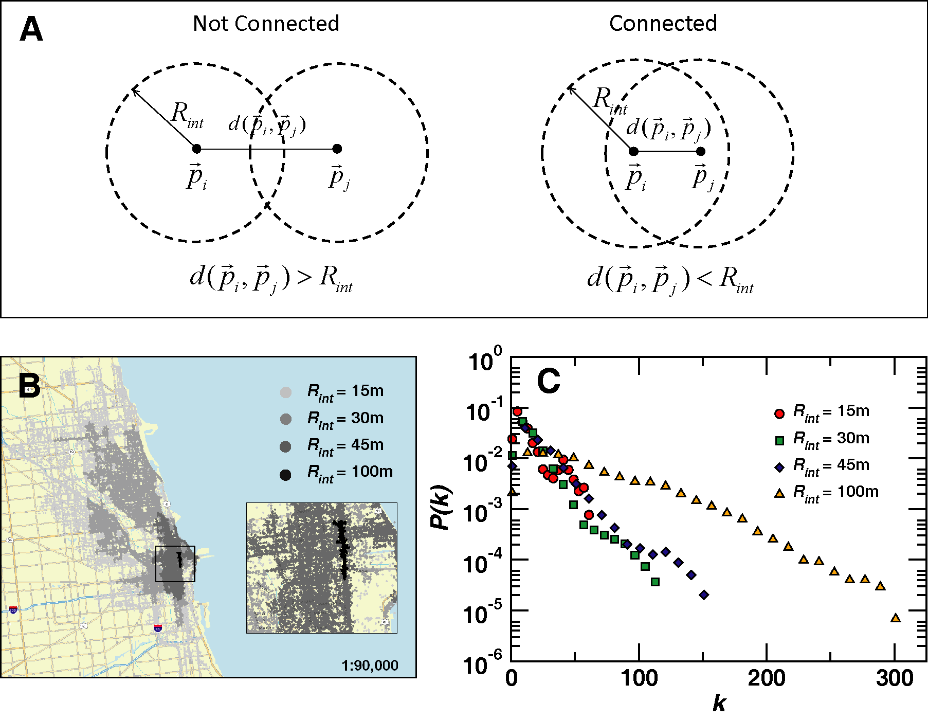
Figure 1.

Figure 1:

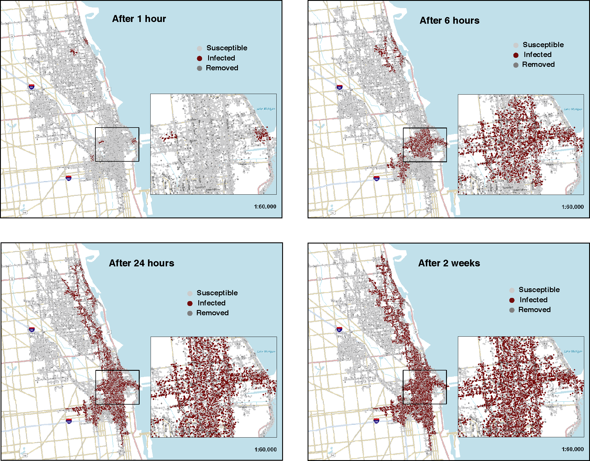
Figure 2:

Figure 2.

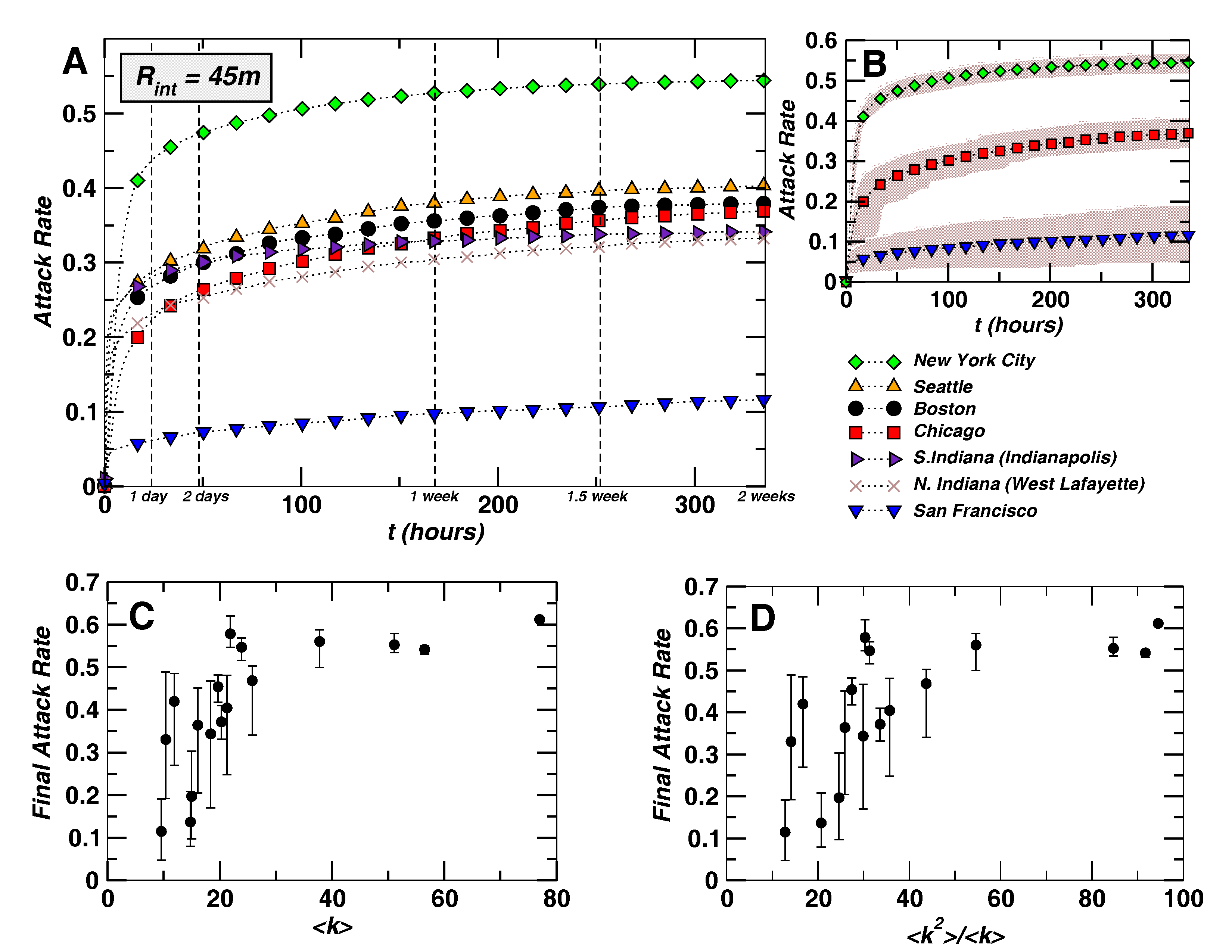
Figure 3:

Figure 3.

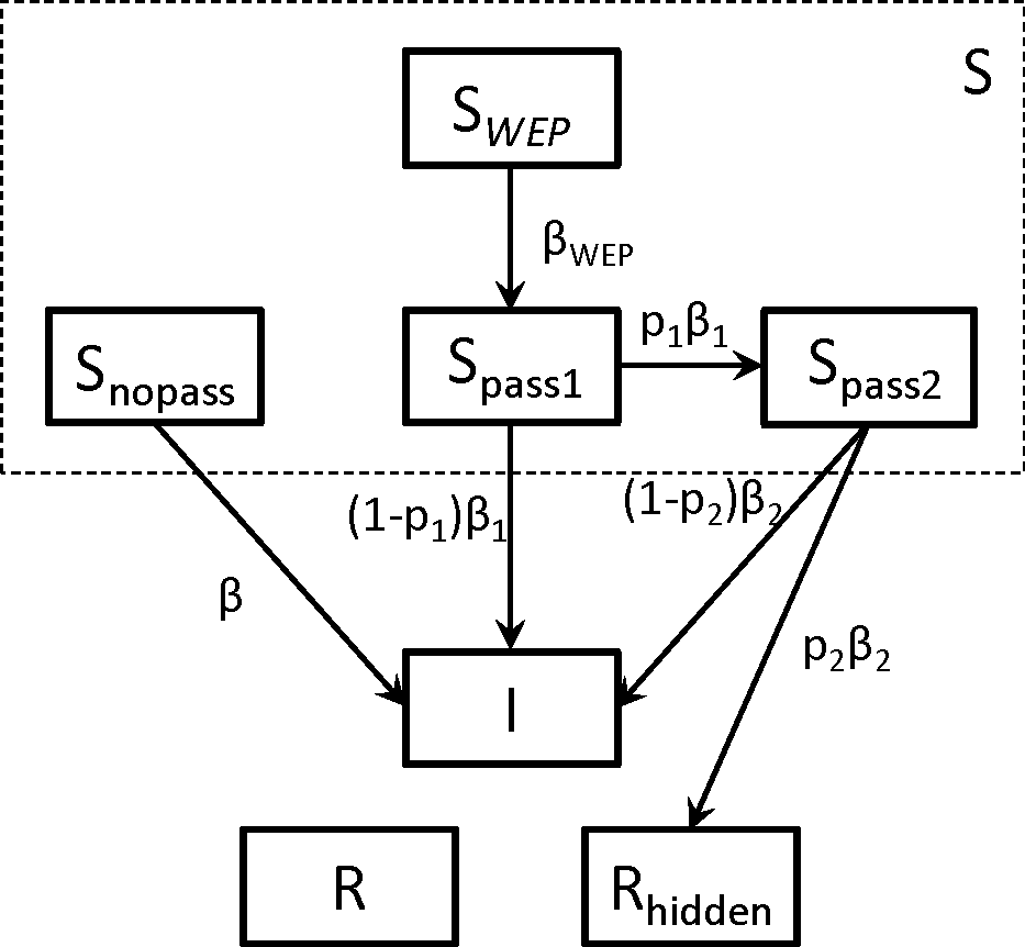
Figure 4:

Figure 4.

References

-
1
Mercer, D. (2006) Home Network Adoption: Wi-Fi Emerges As Mass
Market Phenomenon
(Market Report).
http://www.strategyanalytics.net/default.aspx?mod=ReportAbstract Viewer&%a0=2909. -
2
Telecoms Europe website. (2007)
Wi-fi chipset shipments reach 200m in 2006 – report.
http://www.telecomseurope.net/article.php?id_article=3549. - 3 Stamm, S., Ramzan, Z., and Jakobsson, M. (2006) Drive-by pharming (Technical Report 641, Indiana University).
- 4 Ollmann, G. (2006) The pharming guide (Technical report, Next Generation Security Software Ltd.).
- 5 Jakobsson, M. and Myers, S. editors. (2007) Phishing and Countermeasures: Undertanding the Increasing Problem of Electronic Identity Theft (Wiley).
-
6
Soghoian, C. (2007) A deceit-augmented man in the middle attack
against Bank of
America’s SiteKey service.
http://paranoia.dubfire.net/2007/04/deceit-augmented-man-in-middle-attack.html. - 7 Myers, S. and Stamm, S. (2007) Trawler phishing (Submitted to Computer and Communications Security Conference).
- 8 Tsow, A., Jakobsson, M., Yang, L. and Wetzel, S. (2006) Journal of Digital Forensic Practice, 1, Special Issue 3.
- 9 Bittau, A., Handley, M. and Lackey, J. (2006) SP ’06: Proceedings of the 2006 IEEE Symposium on Security and Privacy (S&P’06) (Washington, DC, USA. IEEE Computer Society), 386 – 400
- 10 Dall, J. and Christensen, M. (2002) Phys. Rev. E, 66, 016121.
- 11 Nemeth, G. and Vattay, G. (2003) Phys. Rev. E, 67, 036110.
- 12 Herrmann, C., Barthélemy, M. and Provero, P. (2003) Phys. Rev. E, 68, 026128.
- 13 Helmy, A. (2003) IEEE Comm. Lett., 7, 490 – 492.
- 14 Molloy, M. and Reed B. (1995) Random Struct Alg., 6, 161 – 179.
- 15 Bollobas, B. and Riordan, O. (2006) Percolation (Cambridge University Press).
- 16 WiGLE: Wireless Geographic Logging Engine. http://www.wigle.net/.
-
17
WiGLE General Stats, first accessed on Febrary, 2007.
http://www.wigle.net/gps/gps/main/stats/. - 18 Gast, M. (2005) 802.11 Wireless Networks: The Definitive Guide, Second Edition (O’Reilly).
- 19 Klein, D. V. (1990) Proceedings of the second USENIX Workshop on Security, 5 – 14.
-
20
Jeff, J., Alan, Y., Ross, B. and Alasdair, A. (2000) The
memorability and security of passwords – some empirical results
(Technical
Report No. 500, Computer Laboratory, University of Cambridge).
http://www.ftp.cl.cam.ac.uk/ftp/users/rja14/tr500.pdf - 21 Anderson, R. M. and May, R. M. (1992) Infectious Diseases of Humans: Dynamics and Control (Oxford Univ. Press, Oxford).
- 22 Watts, D. J. and Strogatz, S. H. (1998) Nature, 393, 440 – 442.
- 23 Barabási, A. L. and Albert, R. (1999) Science, 286, 509 – 512.
- 24 Keeling, M. J. (1999) Proc. R. Soc. Lond. B, 266, 859 – 867.
- 25 Moore, C. and Newman, M. E. J. (2000) Phys. Rev. E, 61, 5678 – 5682.
- 26 Pastor-Satorras, R. and Vespignani, A. (2001) Phys. Rev. Lett., 86, 3200 – 3203.
- 27 Grassberger, P. (1983) Math. Biosci., 63, 157 –172.
- 28 Ben-Avraham, B. and Havlin, S. (2000) Diffusion and Reactions in Fractals and Disordered Systems (Cambridge University Press).
- 29 Cohen, R., Erez, K., Ben-Avraham, D. and Havlin, S. (2000) Phys. Rev. Lett., 85, 4626 – 4628.
- 30 Callaway, D. S., Newman, M. E. J., Strogatz, S. H. and Watts, D. J. (2000) Phys. Rev. Lett., 85, 5468 – 5471.
- 31 Lloyd, A. L. and May, R. M. (2001) Science, 292,1316 – 1317.
- 32 Wardriving. http://www.wardriving.com/.