Series expansion for the density of states of the Ising and Potts models

1. Introduction

The Lentz-Ising model of ferromagnetism has been thoroughly studied since its conception in the 1920’s[Len20]. It was solved in the 1-dimensional case by Ising himself in 1925[Isi25] and in the 2-dimensional case without an external field by Onsager in 1944[Ons44]. For an introduction to the model, see Cipra [Cip87].

The partition function on a graph $G$ on $n$ vertices and $m$ edges is defined as

(1) $$Z(G;x,y)=\sum_{i,j}a_{ij}x^{i}y^{j}.$$

Here $a_{ij}$ counts the number of induced subgraphs of $G$ with $(n-j)/2$ vertices and $(m-i)/2$ edges in the boundary. We refer to the index $i$ as the energy and the index $j$ as the magnetization.

The traditional partition function studied in statistical physics is then obtained by evaluating it at a certain point

(2) $$Z\left(G;e^{K},e^{H}\right)$$

where $K=-J/k_{B}T$, $H=-h/k_{B}T$ and $J$ and $h$ are parameters describing the interaction through edges and with an external magnetic field respectively, $T$ is the temperature and $k_{B}$ the Boltzmann constant.

The main goal in the study of the Ising model on a graph $G$, or some family of graphs, is usually to study the model in the vicinity of a critical temperature, denoted $T_{c}$, where the model undergoes a phase transition and there determine the behaviour of various critical properties.

2. Definitions and notation

Let $G=(V,E)$ be a graph with vertex set $V$ with $|V|=n$ vertices and edge set $E$ with $|E|=m$ edges. Let a state $\sigma$ be a function from the vertices $V$ to the set $\{\pm 1\}$ and let $\Omega$ be the set of all states. We can then define the energy of the graph $G=(V,E)$ in state $\sigma$ to be

(3) $$\mathcal{E}(G,\sigma)=\sum_{uv\in E}\sigma(u)\sigma(v)$$

the magnetization to be

(4) $$\mathcal{M}(G,\sigma)=\sum_{v\in V}\sigma(v)$$

and formulate a generating function that counts them all as

(5) $$Z(G;x,y)=\sum_{\sigma\in\Omega}x^{\mathcal{E}(G,\sigma)}y^{\mathcal{M}(G,\sigma)}=\sum_{ij}a_{ij}x^{i}y^{j}$$

where the last equality defines the coefficients $a_{ij}=a_{ij}(G)$. We often drop $G$ when we can deduce the graph from the context.

We will also need these definitions later:

Definition 1 (T-join).

A T-join $(T,A)$ in a graph $G=(V,E)$ is a subset $T\subseteq V$ of vertices and a subset $A\subseteq E$ of edges such that each vertex in $T$ is incident with an odd number of edges in $A$ and each vertex in $V\setminus T$ is incident with an even number of edges from $A$.

Observe that the cardinality of $T$ has to be even since we can not have a subgraph with an odd number of vertices of odd degree.

Definition 2 (Cut).

A cut $[S,\bar{S}]$ in a graph $G=(V,E)$ is a subset of edges, induced by a partition $S\cup\bar{S}=V$, that have one endpoint in $S$ and the other in $\bar{S}$. Let $|[S,\bar{S}]|$ be the number of edges in the cut.

Definition 3 (Locally vertex transitive).

We say that a sequence of graphs $\{G_{i}\}_{i=1}^{\infty}$ are locally vertex transitive if for each $R$ there exists an $N$ such that all balls of radius $R$, in the graph metric, around each vertex in each graph in the subsequence $\{G_{i}\}_{i=N}^{\infty}$ are isomorphic.

3. Series expansion

We can try to make our problem simpler by setting $y=1$ and get

(6) $$Z(x,1)=Z(x)=\sum_{ij}a_{ij}x^{i}1^{j}=\sum_{i}a_{i}x^{i}$$

where once again the last equality is the definition of the $a_{i}$ coefficients. What do these coefficients count? Since the state $\sigma$ partitions the vertex set $V$ in two parts and the $\mathcal{E}(G,\sigma)$ counts edges with one vertex in one part and the other vertex in the other part as negative and the other edges as positive we get that $a_{i}$ is twice the number of cuts of size $\tfrac{m-i}{2}$ (we count each cut twice since we can interchange the partitions). This has a natural reformulation using even subgraphs, namely:

Theorem 4 (van der Waarden).

Let $a_{i}$ be the number of cuts of size $\tfrac{m-i}{2}$ and let $b_{i}$ be the number of even subgraphs with $i$ edges, then:

(7) $$\sum_{i}a_{i}e^{iK}=2\cosh^{m}K\sum_{i}b_{i}\tanh^{i}K$$

Proof.

The first sum in (7) is the moment generating function for the sequence $a_{i}$. The $k^{\rm th}$ moment of $a_{i}$ can be written as

(8) $$\mu_{k}=\sum_{i}a_{i}i^{k}=\sum_{\sigma\in\Omega}\left(\sum_{uv\in E}\sigma(u)\sigma(v)\right)^{k}$$

We now expand the multinomial $\left(\sum_{uv\in E}\sigma(u)\sigma(v)\right)^{k}$ where each term can be seen as an choice of $k$ out of $m$ edges (not necessarily distinct). Now observe that if we have chosen an even number of edges incident with a vertex, $v$ say, we will have an even number of $\sigma(v)$’s in the product so they contribute $+1$. If we have chosen an odd number of vertices we can find a smallest (in some arbitrarily order) such odd vertex $v$ and we see that if we change the state $\sigma$ to the state $\sigma^{\prime}$ with $\sigma(v)=-\sigma^{\prime}(v)$ and all other values equal, we will get a bijection between states witch contribute $+1$ and $-1$ and with at least one vertex of odd degree. Our conclusion is that we only count the choices where we have an even degree at each vertex. We will however count subgraphs where we have the opportunity to choose each edge a multiple number of times. If we reduce the multiple edges modulo 2 we get a simple subgraph of even degree. The “surviving” edges are the ones that where chosen an odd number of times so an even number of those “odd” edges have to be incident at each vertex.

If we now change our view and instead of adding up the $k$ moments, change the order of summation, and add up along the index of the number of “surviving” odd edges $i$ we get a simple connection between the simple subgraphs and subgraphs with multiple edges. We can construct an even multiedge subgraph by first select a simple subgraph with even degree at each vertex and then multiply each edge an odd number of times and then select a number of edges not in the even subgraph to multiply an even number of times. So if we first choose an even subgraph with $i$ edges and multiply each edge an odd number of times we get the generating function $b_{i}\sinh^{i}K$, and then choose a number of edges outside the even subgraph and multiply these an even number of times, we get the generating function $\cosh^{m-i}K$, and we end up with an multiedge subgraph with an even number of edges incident to each vertex. If we now sum over all $i$ we get

(9) $$\sum_{i}b_{i}\sinh^{j}K\cosh^{m-i}K=\cosh^{m}K\sum_{i}b_{i}\tanh^{i}K$$

and we see each of these graphs twice and therefor this gives (7). ∎

To formulate the full two variable connection we need T-joins instead of even degree subgraphs and also consider the size of the sets in the vertex partition induced by the state. Also note that in this theorem we have slightly changed the meaning of $a_{ij}$ and $b_{ij}$ to make the proof using standard graph theoretic notation. The following theorem can be found in e.g. [Big77]:

Theorem 5.

Let $G=G(V,E)$ be a graph, $a_{ij}$ the number of cuts $[S,\bar{S}]$ with $|[S,\bar{S}]|=i$ and $|S|=j$. Let $b_{ij}$ be the number of T-joins $(T,A)$ with $|A|=i$ and $|T|=j$. Then

$$\sum_{ij}b_{ij}x^{i}y^{j}=2^{-|V|}\sum_{ij}a_{ij}(1-x)^{i}(1+x)^{|E|-i}(1-y)^{j}(1+y)^{|V|-j}$$

Proof.

Fix a subset $T\subseteq V$ of vertices and a subset $A\subseteq E$ of edges from the graph $G=G(V,E)$. Let $S\subseteq V$ be another subset of vertices and $[S,\bar{S}]$ be the cut defined by the edges from $S$ to $\bar{S}=V\setminus S$. Let the weight of the vertices in $T\cap S$ be $-y$, the weight of the vertices in $T\cap\bar{S}$ be $y$, the weight of the edges from $A$ that lies in the cut $[S,\bar{S}]$ be $-x$ and the rest of the edges from $A$ have weight $x$. Let the total weight of $(T,A)$ with respect to the cut $[S,\bar{S}]$ be the product of the weights of the edges and vertices in $(T,A)$. We say that the weight is positive if the coefficient in front of $x^{|A|}y^{|T|}$ is positive and negative otherwise. By magnitude we denote the weight without the sign.

$(T,A)$ can fail to be a T-join in basically three ways. First the cardinality of $T$ can be odd, secondly there can exist a smallest vertex (in an arbitrary order of the vertices) $v$ that is incident with an odd number of edges from $A$ and does not belong to $T$, and finally there can exist a smallest vertex $v$ that is incident with an even number of edges from $A$ and belongs to $T$.

In the first case we have two cuts $[S,\bar{S}]$ and $[\bar{S},S]$ in which the magnitude of the weight will be the same but with opposite sign.

In the two latter cases we have a bijection between cuts with $v\in S$ and $v\notin S$ (we simply move the vertex $v$ between $S$ and $\bar{S}$) that once again give the same magnitude and different signs of the weight. If we sum over all cuts the total contribution of such a choice of $(T,A)$ will cancel.

If $(T,A)$ indeed is a T-join the weight will always be positive since we either have an even number of vertices in $T\cap S$ and an even number of edges crossing the cut or an odd number of vertices in $T\cap S$ and an odd number of vertices crossing the cut. All in all we end up with an even number of minus signs and thus a positive weight.

If we now sum over all choices $(T,A)$ and $S$ we will count each T-join $2^{|V|}$ times. If we rearrange our summation (i.e. we first choose a cut and then go through all choices of $T$ and $A$) we get the theorem. ∎

To get Theorem 4 we have to shift the indices and substitute $x$ for $e^{-2K}$ and $y$ for 0 and finally double all values since we count all cuts twice in (7).

(10) $$2e^{mK}\sum_{i,j}a_{ij}e^{-2iK}0^{j}=[\text{since $0^{0}=1$}]=\sum_{i}2a_{i}e^{(m-2i)K}=\\ 2e^{mK}2^{-m}\sum_{i,j}b_{ij}(1-e^{-2K})^{i}(1+e^{-2K})^{m-i}1^{n}=\\ 2\left(\frac{e^{K}+e^{-K}}{2}\right)^{m}\sum_{i}b_{i}\left(\frac{1-e^{-2K}}{1+e^{-2K}}\right)^{i}=\\ 2\cosh^{m}K\sum_{i}b_{i}\tanh^{i}K$$

where $b_{i}$ denotes the number of T-joins with $i$ edges. Now, since $a_{i}$ counts the number of cuts with $i$ edges in Theorem 5, $2a_{i}e^{(m-2i)K}$ corresponds to the $a_{i}e^{iK}$ in Theorem 4 via reindexing and the fact that each cut is counted twice in Theorem 4.

Since we have a symmetry between T-joins and cuts we have the following corollary:

Corollary 6.

With the same notation as in theorem 5 we have

$$\sum_{i,j}a_{ij}x^{i}y^{j}=2^{-|E|}\sum_{i,j}b_{ij}(1-x)^{i}(1+x)^{|V|-i}(1-y)^{j}(1+y)^{|E|-j}$$

Proof.

If we choose a T-join instead of a cut the weight of $(T,A)$ will always be positive if and only if $(T,A)$ is a cut. In other cases the contributions once again cancel out. ∎

3.1. The thermodynamic limit

In Physics we are interested in the so called thermodynamic limit of a sequence of graphs $\{G_{j}\}_{j=1}^{\infty}$. This is defined as

(11) $$f(x)=\lim_{j\rightarrow\infty}\tfrac{1}{|V(G_{j})|}\log Z(G_{j};x,1)$$

when it exists. An example of such a family is $\{C_{n}\times C_{n}\}_{n=3}^{\infty}$. If the graph family is locally vertex transitive its easy to see that the number of connected T-joins of fixed size will grow proportionally to $|V(G)|$. From that follows that the total number of T-joins of a fixed size will grow as a polynomial with degree equal to the maximal number of connected components in the T-joins of that size and thus will the thermodynamic limit exist.

If we change notation so that our index set instead is the number of vertices $n$ in our graph sequence and use $b_{j}(n)$ to denote the number of T-joins with $j$ edges we see that the thermodynamic limit is

(12) $$\lim_{n\rightarrow\infty}\tfrac{1}{n}\log 2\cosh^{m}x\sum_{j}b_{j}(n)\tanh^{j}x=\log 2+d\cosh x+\sum_{j}b_{j}\tanh^{j}x$$

which defines a new set of $b_{j}$:s that happens to be rational numbers and $d=m/n$, the average degree.

3.2. Taylor series

It can be of interest to plot these functions, or at least some approximation of them. Since we have a phase transition in all interesting cases its hard to find one function that works for the entire interval. In this section we will instead develop two Taylor approximations, one for the high-temperature case and one for the low-temperature case. The first one is simple, take

(13) $$u(K)=\sum_{i}a_{i}K^{i}=\log 2+d\log\cosh K+\lim_{n\rightarrow\infty}\tfrac{1}{n}\log\sum_{i}b_{i}(n)\tanh^{i}K$$

and Taylor expand around $K=0$. If you want the function $K(u)$ you can invert $u(K)$ as a Taylor series. Its often better to plot a Padé-approximation of $u(K)$. The second one needs a little more work:

(14) $$\frac{\mathrm{d}}{\mathrm{d}K}u(K)=\frac{\mathrm{d}}{\mathrm{d}K}\left[\log 2+d\log\cosh K+\lim_{n\rightarrow\infty}\tfrac{1}{n}\log\sum_{i}b_{i}(n)\tanh^{i}K\right]=\\ \left[\begin{array}[]{rl}x=&\tanh K\\ \tfrac{\mathrm{d}}{\mathrm{d}K}=&(1-x^{2})\tfrac{\mathrm{d}}{\mathrm{d}x}\end{array}\right]=dx+(1-x^{2})\frac{\mathrm{d}}{\mathrm{d}x}\lim_{n\rightarrow\infty}\tfrac{1}{n}\log\sum_{i}b_{i}(n)x^{i}=\\ dx+(1-x^{2})\frac{\mathrm{d}}{\mathrm{d}x}\lim_{n\rightarrow\infty}\tfrac{1}{n}\log\tfrac{1}{2^{n}}\sum_{i}a_{m-2i}(n)(1-x)^{i}(1+x)^{m-i}=\\ dx+(1-x^{2})\frac{\mathrm{d}}{\mathrm{d}x}\lim_{n\rightarrow\infty}\left[-\log 2+d\log(1+x)+\tfrac{1}{n}\log\exp\left(n\sum_{i}a_{i}\left(\frac{1-x}{1+x}\right)^{i}\right)\right]=\\ dx+\frac{d(1-x^{2})}{1+x}+(1-x^{2})\frac{\mathrm{d}}{\mathrm{d}x}\sum a_{i}\left(\frac{1-x}{1+x}\right)^{i}=d+(1-x^{2})\frac{\mathrm{d}}{\mathrm{d}x}\sum a_{i}\left(\frac{1-x}{1+x}\right)^{i}=\\ d+\frac{2(x-1)}{(x+1)}\sum a_{i}\left(\frac{1-x}{1+x}\right)^{i-1}=d-2\sum a_{i}\left(\frac{1-x}{1+x}\right)^{i}=\\ d-2\sum a_{i}\left(\frac{1-\tanh K}{1+\tanh K}\right)^{i}$$

By not doing the last substitution $x=\tanh K$ its easy to invert this function and plot it in the low temperature (high energy) portion of the scale.

4. Two other series expansions

From the basic thermodynamic limit one can construct two other sequences that are of a more combinatorial flavour. These are sequences with integer coefficients. This is because they, instead of weighting the counts, make an explicit order in which you have to choose things and thus avoid dividing with large factorials. The correspondence with the thermodynamic limit series are:

(15) $$\sum_{i\geq 0}b_{i}(n)x^{i}=\exp\left(n\sum_{i\geq 1}b_{i}x^{i}\right)=\prod_{i\geq 1}\left(\frac{1}{1-x^{i}}\right)^{n\beta_{i}}=\prod_{i\geq 1}\left(\frac{1}{1-\widehat{\beta}_{i}x^{i}}\right)^{n}$$

The coefficients are connected trough these simple triangular linear equations:

(16) $$ib_{i} =\sum_{t|i}t\beta_{t}$$

(17) $$ib_{i} =\sum_{rs=i}r\widehat{\beta}^{s}_{r}$$

(18) $$i\beta_{i} =\sum_{rst=i}\mu(r)t\widehat{\beta}^{s}_{t}$$

4.1. What they are counting

The new series can be seen as placing connected subgraphs at each vertex in some order. First we place all subgraphs (including the empty one) rooted at vertex one, then the subgraphs rooted at vertex two and so on in such a way that we never form a new connected component. In this way we avoid symmetries and we get a integer sequence. We can still calculate, in principle, the different $\beta_{i}$ and $\widehat{\beta}_{i}$ for locally vertex transitive graphs.

5. Plots

We shall now compare these Taylor expansions of the series with some sampled data to compare how well behaved the series are around the critical energy. As we shall see, the series are rather far from what can be expected to be the truth.

5.1. Simple cubic lattice

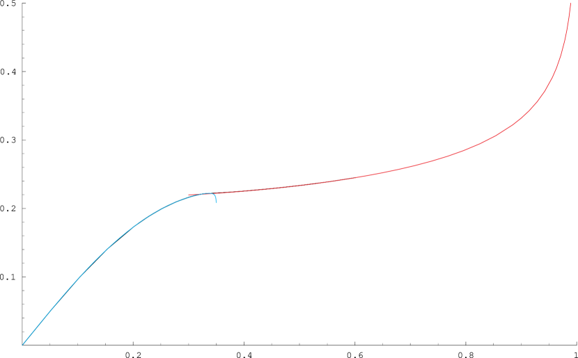
Figure 1. $K(u)$ for the three-dimensional simple cubic lattice together with sampled data for the cubes of linear order 32, 64 and 128.

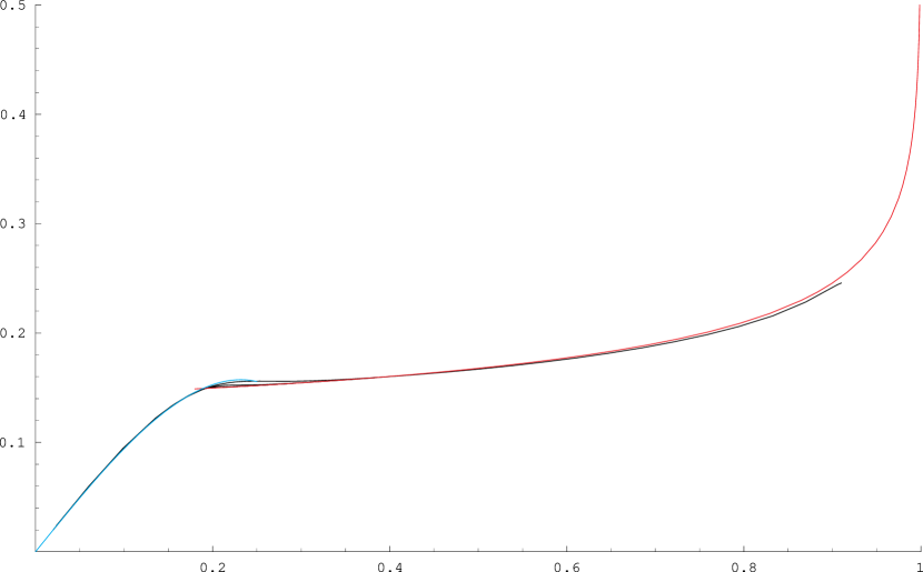
Figure 2. $K(u)$ for the four-dimensional simple cubic lattice together with sampled data for the cube of linear order 4, 6, 8, 12, 16, 32, 48 and 64.

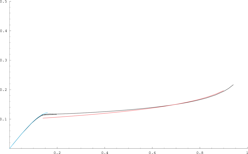
Figure 3. $K(u)$ for the five-dimensional simple cubic lattice together with sampled data for the cube of linear order 4, 6, 8, 12, 16 and 32.

We start of with the simple cubic lattice in three, four and five dimensions. As can be expected, the longest series expansion is for the three-dimensional simple cubic lattice. The four- and five-dimensional simple cubic lattices have much shorter high- and low-temperature expansions. Figure 1 to 3 shows $K(u)$ curves for the three lattices respectively. The pictures are of diagonal Padé-approximants of the Taylor expansions. The Padé-approximant for the function of the three-dimensional simple cubic lattice is fairly accurate to about $K\approx.22$. For the four- and five-dimensional lattices the accuracy is a lot lower as can be seen from the pictures.

6. Guessing the radius of convergence

The interesting part is of course to try to find the radius of convergence for the series of the function $u(K)$ since that would give the critical temperature $K_{c}$. A fairly good guess for $K_{c}$ for the simple cubic lattice is that it is approximately $0.2216546$ (see e.g. [HRL⁺]). A simple observation is that the radius of convergence must be smaller than any $1/\widehat{\beta_{i}}^{1/i}$ since otherwise the infinite product (15) will not converge. In Table 1 the row labelled $\min$ is the minimum over all known values of $\widehat{\beta_{i}}$ for the simple cubic lattice. In trying to extrapolate this value we have used a polynomial of degree 3 and a min square approximation to the data set $(1/i,1/\widehat{\beta_{i}}^{1/i})$ and looked at the constant term in the resulting polynomial. This gives the result in the row labelled $f(0)$. Since the coefficients is some form of combinatorial quantity it is not unthinkable that they grow exponentially. We have thus also tried to fit the data $(i,\widehat{\beta_{i}})$ to the functions $\alpha^{i}i^{\beta}\gamma$ and $\alpha^{i}\gamma$ and calculated $1/\alpha$ that gives us the guessed radius of convergence. This is the last two lines of Table 1. The second column is the same thing for the coefficients of $b_{i}$. When we come to the low temperature part we get into some trouble since the coefficients of the sequences $a_{i}$ and $\widehat{\alpha_{i}}$ have both positive and negative signs. If we try to use the same analysis as for the (all positive) $b_{i}$ and $\widehat{\beta_{i}}$, we get very erratic numbers, so instead we split the sequences in a positive and a negative part and do the analysis separately. As observed by others, the low temperature series seems to have a complex root that is closer to the origin than the physically important real root. Fortunately does the extrapolation with $\alpha^{i}i^{\beta}\gamma$ for the $b_{i}$ and $\widehat{\beta_{i}}$ series give a decent idea of what the critical temperature may be.

	$\widehat{\beta_{i}}$	$b_{i}$	$\widehat{\alpha_{i}}^{+}$	$\widehat{\alpha_{i}}^{-}$	$a_{i}^{+}$	$a_{i}^{-}$
$\min$	0.291989	0.291989	0.618531	0.616299	0.618531	0.616307
$f(0)$	0.227727	0.227839	0.54278	0.543852	0.542846	0.539196
$\alpha^{i}i^{\beta}\gamma$	0.221418	0.221451	0.523726	0.520324	0.523747	0.542904
$\alpha^{i}\gamma$	0.258385	0.258429	0.578131	0.565115	0.578137	0.56453

Table 1. Different ways to try to guess the radius of convergence for the simple cubic lattice.

Appendix A Tables

We have collected the various series we have found in this appendix. Some of these are old and thus not especially long and some are from newer calculations and longer.

$n$	$\alpha_{n}$	$\widehat{\alpha}_{n}$	$a_{n}$
6	1	1	1
10	3	3	3
12	-4	-4	-7/2
14	15	15	15
16	-33	-33	-33
18	104	104	313/3
20	-282	-285	-561/2
22	849	849	849
24	-2460	-2470	-9847/4
26	7485	7485	7485
28	-22542	-22647	-45069/2
30	69392	69384	346966/5
32	-213738	-214299	-427509/2
34	666750	666750	666750
36	-2086785	-2092121	-12520405/6
38	6583341	6583341	6583341
40	-20852223	-20892996	-83409453/4
42	66425750	66424630	464980286/7
44	-212410377	-212770353	-424819905/2
46	682202205	682202205	682202205
48	-2198562644	-2201602421	-17588511087/8
50	7110521070	7110521022	35552605353/5
52	-23065955826	-23093964696	-46131904167/2
54	75045653088	75045278168	675410878105/9
56	-244806881325	-245063348553	-979227570369/4
58	800606679471	800606679471	800606679471
60	-2624325216574	-2626724535242	-13121625909861/5
62	8621219166681	8621219166681	8621219166681
64	-28379404026078	-28402366460136	-113517616531821/4

Table 2. Simple cubic lattice

Table 3. Simple cubic lattice

Table 4. Simple cubic lattice in dimension 4 ($x^{4}_{n}$) and 5 ($x^{5}_{n}$)

Table 5. Simple cubic lattice, 3-states Potts model

References

- [Big77] Norman Biggs. Interaction models. Cambridge University Press, Cambridge, 1977. Course given at Royal Holloway College, University of London, October–December 1976, London Mathematical Society Lecture Note Series, No. 30.
- [Cip87] Barry A. Cipra. An introduction to the Ising model. Amer. Math. Monthly, 94(10):937–959, 1987.
- [HRL+] Roland Häggkvist, Andres Rosengren, Per Håkan Lundow, Klas Markström, Daniel Andrén, and Petras Kundrotas. On the Ising model for the simple cubic lattice. Manuscript.
- [Isi25] Ernst Ising. Beitrag zur Theorie des Ferromagnetismus. Z.Physik, 31:253–258, 1925.
- [Len20] Wilhelm Lenz. Beitrag zum Verständnis der magnetishen Erscheinungen in festen Körpern. Z. Physik, 21:613–615, 1920.
- [Ons44] Lars Onsager. Crystal statistics. I. A two-dimensional model with an order-disorder transition. Phys. Rev. (2), 65:117–149, 1944.