Entropy of Schwarzschild Black Holes on DGP Brane

Abstract

We study the entropy of Schwarzschild black holes on DGP brane. The radius of event horizon on DGP brane is obtained by a numerical method. It is smaller than that of Einstein gravity in the conventional branch, and is larger in the accelerated branch. However, the difference is very small. The entropy of the black hole is calculated by using the improved brick-wall method.

After Bekenstein has suggested that the entropy of a black hole is proportional to the surface area at the event horizon bekenstein , there have been several studies for the statistical origin of the entropyhawking ; zt ; fn . This can be understood by using a brick-wall methodthooft or an improved brick-wall methodhzk ; kpsy . In the improved brick-wall method, a thin layer at the horizon is used instead of an infinite spherical box. As for a black hole on the Dvali-Gabadadze-Porrati(DGP) modeldgp , an exact expression of metric has not been obtained. In this paper, we first get the radius of event horizon numerically, then, based on this data about horizon, calculate the entropy of the black hole by using an improved brick-wall method.

The action in the DGP model is given bydgp

$$S=M_{*}^{3}\int d^{5}x\sqrt{-g}R+M_{P}^{2}\int d^{4}x\sqrt{-\tilde{g}}\tilde{R}$$ (1)

where the tilde denotes the quantities on the four-dimensional world-volume of the brane. A cross-over scale is defined by $r_{c}=m_{c}^{-1}=M_{P}^{2}/(2M_{*}^{3})$. We consider a spherically symmetric and static black hole on the brane. Then, the five-dimensional line element can be written as

$$ds_{(5)}^{2}=-e^{-\lambda}dt^{2}+e^{\lambda}dr^{2}+r^{2}d\Omega^{2}+\gamma drdy+e^{\sigma}dy^{2},$$ (2)

where $\lambda$, $\gamma$, and $\sigma$ are functions only for $r$ and $y$ and the brane is located at $y=0$. The equations of motion from the action (1) with Israel’s junction conditions reduce to the equation for $\lambda$ on the brane as followsgi:prd :

$$U^{2}_{z}-4(1+U)U_{z}-8U(2+U)=0,$$ (3)

where $z=\ln(r/r_{0})$, $U=-2\exp(-2z)P_{r}/3m^{2}_{c}r^{2}_{0}$, $P_{r}=dP/dr$, and $P(r)=r(1-\exp(-\lambda))|_{y=0}$ ($r_{0}$ being an arbitrary constant). Two solutions of Eq. (3), regular (or conventional) and accelerated branches, are given bygi:prd

$$k_{1}r\!\! = \!\!R(U)=\left[-\frac{(1+3U+f)}{U^{2}(3+3U+\sqrt{3}f)^{2\sqrt{3}}(-5-3U+f)}\right]^{\frac{1}{8}},$$ (4)

$$k_{2}r\!\! = \!\!A(U)=\left[-\frac{(-5-3U+f)(-3-3U-\sqrt{3}f)^{2\sqrt{3}}}{(U+2)^{2}(1+3U+f)}\right]^{\frac{1}{8}},$$ (5)

where $k_{1}$ and $k_{2}$ are constants of integration and $f=\sqrt{1+6U+3U^{2}}$. By applying boundary conditions by $P(0)=r_{M}$ and $P(\infty)=0$ in the regular branch and $P(0)=r_{M}$ and $P(r)\approx m^{2}_{c}r^{3}$ for large $r$ in the accelerated branch, $k_{1}$ and $k_{2}$ are determined as $2(r_{*}k_{1})^{3}=c_{1}\approx 0.43$ and $2(r_{*}k_{2})^{3}=c_{2}\approx 4.41$, where $r_{*}=(r_{M}r^{2}_{c})^{1/3}$gi:plb . From $P(r)=-\frac{3}{2}m^{2}_{c}\int dr\ r^{2}U(r)$, we obtain

$$P(r)\!\! = \!\!r_{M}\left[1-\frac{1}{c_{1}}UR(U)^{3}-\frac{1}{c_{1}}\int_{U}^{\infty}\!dUR(U)^{3}\right],$$ (6)

$$P(r)\!\! = \!\!r_{M}\left[1-\frac{1}{c_{2}}UA(U)^{3}+\frac{1}{c_{2}}\int_{-\infty}^{U}\!dUA(U)^{3}\right],$$ (7)

which correspond to the regular and accelerated branches, respectively.

Since $P(r_{H})=r_{H}$ at the horizon, we can obtain $U_{H}\equiv U(r_{H})$ from Eqs. (4) – (7). Substituting the corresponding $U_{H}$’s into Eqs. (4) and (5), the horizons are calculated from $r_{H}/r_{M}=\left[2(r_{c}/r_{M})^{2}/c_{1}\right]^{1/3}R(U_{H})$ for the regular branch and $r_{H}/r_{M}=\left[2(r_{c}/r_{M})^{2}/c_{2}\right]^{1/3}A(U_{H})$ for the accelerated branch. The results for the regular and the accelerated branches are shown in Fig. 1. Note that the horizon can be written as $r_{H}=r_{M}+\xi$, where $\xi$ should be very small because $r_{c}/r_{M}$ is very large. This fact will be taken into account for calculating the entropy.

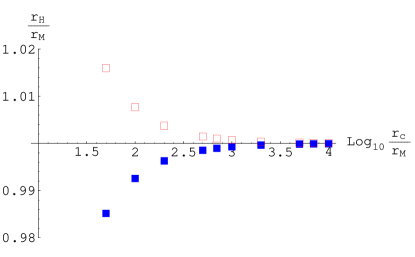
Figure 1: Filled boxes and unfilled boxes are the ratios of $r_{H}$ to $r_{M}$ in the regular and the accelerated branches, respectively, where $r_{H}$ is a horizon of a black hole on DGP brane and $r_{M}$ is a horizon of a Schwarzschild black hole in Einstein gravity. It shows that $r_{H}$ approaches $r_{M}$ when $r_{c}$ is much larger than $r_{M}$.

In order to find the entropy of a black hole, we would rewrite the line element (2) on the brane as $ds^{2}=-fdt^{2}+f^{-1}dr^{2}+r^{2}d\Omega^{2}$, where $d\Omega$ denotes a solid angle. The asymptotic behavior of the metric is obtained as

$$f(r) \approx 1-\frac{r_{M}}{r}+b\alpha m_{c}^{2}r^{2}\left(\frac{r_{\ast}}{r}\right)^{2(\sqrt{3}-1)},\ \textrm{for $r\ll r_{\ast}$}$$ (8)

$$f(r) \approx 1-\frac{\tilde{r}_{M}^{2}}{r^{2}}-bm_{c}^{2}r^{2},\qquad\qquad\qquad\ \textrm{for $r\gg r_{\ast}$}$$ (9)

where $\alpha\approx 0.84$ and $b=1$ and $b=-1$ correspond to the conventional branch and the accelerated branch, respectively, gi:prd ; gi:plb .

Since $a\equiv b\alpha m_{c}^{2}r_{*}^{2(\sqrt{3}-1)}$ is very small, there exists a solution $r_{H}$ such that $f(r_{H})=0$, where $r_{H}=r_{M}+\xi$ with $|\xi|\ll r_{M}$. The fact that $\xi$ is very small compared to $r_{M}$ appears in Fig. 1. From $f(r_{H})=f(r_{M}+\xi)=0$, we obtain $\xi\approx-ar_{M}^{5-2\sqrt{3}}$. Note that the radius of the event horizon is smaller than that of Einstein gravity in the conventional branch, and it is larger in the accelerated branch. Now, the Hawking temperature is given by $T=\beta^{-1}=\kappa/(2\pi)\approx\gamma/(4\pi r_{H})$, where $\kappa$ is a surface gravity of the black hole and $\gamma\equiv 1-\xi/r_{H}+(4-2\sqrt{3})ar_{H}^{4-2\sqrt{3}}\approx 1-(5-2\sqrt{3})\xi/r_{H}$.

In order to calculate the entropy of a given system in the brick-wall method, we consider a quantum gas of scalar particles confined within a box near the horizon of a black hole and introduce a cut-off parameterthooft . The free scalar field is assumed to satisfy the Klein-Gordon equation, $(\Box+m^{2})\Psi=0$, with boundary conditions $\Psi(r_{H}+h)=\Psi(L)=0$, where $r_{H}$ is the horizon, $m$ is the mass of a scalar field, $h$ is an infinitesimal cut-off parameter, and $r_{H}+h$ and $L$ represent the inner and the outer walls of a “spherical” box, respectively. Suppose that this system is in thermal equilibrium at a temperature $T$ with an external reservoir. Using $\Psi=\exp(-i\omega t)\psi(r,\theta,\varphi)$, the Klein-Gordon equation is reduced to

$$\frac{\partial^{2}\psi}{\partial r^{2}}+\left(\frac{2}{r}+\frac{1}{f}\frac{\partial f}{\partial r}\right)\frac{\partial\psi}{\partial r}+\frac{1}{f}\left[\frac{\omega^{2}}{f}-m^{2}+\frac{1}{r^{2}}\left(\frac{\partial^{2}}{\partial\theta^{2}}+\cot\theta\frac{\partial}{\partial\theta}+\csc^{2}\theta\frac{\partial^{2}}{\partial\varphi^{2}}\right)\right]\psi=0.$$ (10)

By the WKB approximation, using $\psi\sim\exp[iS(r,\theta,\varphi)]$, we obtain $p_{r}^{2}=f^{-1}[\omega^{2}/f-m^{2}-p_{\theta}^{2}/r^{2}-p_{\varphi}^{2}/(r^{2}\sin^{2}\theta)]$, where $p_{r}=\partial S/\partial r$, $p_{\theta}=\partial S/\partial\theta$, and $p_{\varphi}=\partial S/\partial\varphi$. Then, $p^{2}=g^{rr}p_{r}^{2}+g^{\theta\theta}p_{\theta}^{2}+g^{\varphi\varphi}p_{\varphi}^{2}=\omega^{2}/f-m^{2}$. The number of quantum states with energy not exceeding $\omega$ can be written as

$$n(\omega)=\frac{1}{(2\pi)^{3}}\int drd\theta d\varphi dp_{r}dp_{\theta}dp_{\varphi}=\frac{2}{3\pi}\int dr\,\frac{r^{2}}{\sqrt{f}}\left(\frac{\omega^{2}}{f}-m^{2}\right)^{\frac{3}{2}}.$$ (11)

The free energy is given by

$$F=-\int_{m\sqrt{f}}^{\infty}d\omega\,\frac{n(\omega)}{e^{\beta\omega}-1}=-\frac{2}{3\pi\beta^{4}}\int dr\frac{r^{2}}{f^{2}}\int_{x_{0}}^{\infty}dx\,\frac{(x^{2}-x_{0}^{2})^{3/2}}{e^{x}-1},$$ (12)

where $x=\beta\omega$ and $x_{0}=\beta m\sqrt{f}$.

The degrees of freedom are dominant near horizon. Thus, we consider a thin layer with $L=r_{H}+h+\delta$, where $\delta$ is small. Since $x_{0}$ goes to zero near horizon, we obtain

$$F=-\frac{2}{3\pi\beta^{4}}\int dr\,\frac{r^{2}}{f^{2}}\int_{0}^{\infty}dx\,\frac{x^{3}}{e^{x}-1}\approx-\frac{2\pi^{3}}{45\beta^{4}}\int_{r_{H}+h}^{r_{H}+h+\delta}dr\,\frac{r^{2}}{f^{2}}.$$ (13)

The metric near the horizon can be written as $f(r)\approx\gamma(1-r_{H}/r)$. Therefore, the free energy can be calculated as

$$F\approx-\frac{2\pi^{3}r_{H}^{4}}{45\beta^{4}\gamma^{2}}\frac{\delta}{h(h+\delta)},$$ (14)

and the entropy becomes

$$S=\beta^{2}\frac{\partial F}{\partial\beta}\approx\frac{8\pi^{2}r_{H}^{4}}{45\beta^{2}\gamma^{2}}\frac{\bar{\delta}^{2}}{\bar{h}^{2}(\bar{h}^{2}+\bar{\delta}^{2})},$$ (15)

where $\bar{h}\equiv\int_{r_{H}}^{r_{H}+h}\sqrt{g_{rr}}\,dr$, $\bar{\delta}\equiv\int_{r_{H}+h}^{r_{H}+h+\delta}\sqrt{g_{rr}}\,dr$. Note that $\bar{h}$ and $\bar{\delta}$ are the cut-off parameter and the thickness of the layer, respectively. Thus, we can write the entropy as

$$S\approx\frac{1}{4}{\cal A}\cdot\frac{1}{90\pi}\frac{\bar{\delta}^{2}}{\bar{h}^{2}(\bar{h}^{2}+\bar{\delta}^{2})},$$ (16)

where ${\cal A}=4\pi r_{H}^{2}$. When the cut-off parameter $\bar{h}$ is chosen as $\bar{\delta}^{2}/[\bar{h}^{2}(\bar{h}^{2}+\bar{\delta}^{2})]=90\pi/G$, Eq. (16) agrees with the Bekenstein-Hawking entropy $S_{\rm BH}={\cal A}/4G$bekenstein ; hawking .

One may consider the cut-off introduced in the brick-wall method a bit ad hoc. In Ref.dlm ; kksy , this point was criticized and the Pauli-Villars regularization scheme was used to replace the cut-off. In Refs.jp , the entropy was evaluated based on the notion of entanglement entropy. Below, we evaluate the entropy in the thin layer using the Pauli-Villars scheme and compare it with our result (16). Introducing the five regulator fields ($i=1,\dots,5$) besides the original field ($i=0$)dlm , the total free energy becomes

$$\bar{F}\approx-\frac{2r_{H}^{2}}{3\pi\gamma^{2}}\sum_{i=0}^{5}\Delta_{i}\int_{0}^{\infty}\frac{d\omega}{e^{\beta\omega}-1}\int_{h^{\prime}}^{L^{\prime}}ds\frac{(\omega^{2}-\gamma m_{i}^{2}s)^{3/2}}{s^{2}(1-s)^{4}},$$ (17)

where $\Delta_{0}=\Delta_{3}=\Delta_{4}=+1$ for the commuting fields and $\Delta_{1}=\Delta_{2}=\Delta_{5}=-1$ for the anticommuting fields and the integration is taken for values where the square root is real. Setting $h^{\prime}=0$ and focusing only on the divergent contributions at the horizon, we obtain the entropy

$$\bar{S}\approx\frac{\pi r_{H}^{3}}{3\beta}\left(B+\frac{32\pi^{2}}{15\beta^{2}\gamma^{2}}A\right)=\frac{\cal A}{4}\frac{B\gamma}{12\pi}+\frac{A\gamma}{90},$$ (18)

with the same $A$ and $B$ coefficients given in Ref.dlm . As it was discussed in Ref.dlm , the second term including $A$ corresponds to the 1-loop correction to the quadratic-curvatre terms of the gravitational acton, and is irrelevant to our case. The first term corresponds to the 1-loop renormalization of the Bekenstein-Hawking entropy $S={\cal A}/4G_{R}$, where the renormalized Newton’s constant $G_{R}$ is given by $1/G_{R}=1/G_{B}+B\gamma/12\pi$ with the bare Newton’s constant $G_{B}$. Note that our result slightly differs from the result of Ref.dlm by a factor $\gamma$.

References

• (1) J. D. Bekenstein, Lett. Nuovo. Cim. 4, 737 (1972); Phys. Rev. D 7, 2333 (1973); Phys. Rev. D 9, 3292 (1974).
• (2) S. W. Hawking, Commun. Math. Phys. 43, 199 (1975).
• (3) W. H. Zurek and K. S. Thorne, Phys. Rev. Lett. 54, 2171 (1985).
• (4) V. P. Frolov and I. Novikov, Phys. Rev. D 48, 4545 (1993); V. P. Frolov and D. V. Fursaev, Phys. Rev. D 61, 024007 (1999).
• (5) G. ’t Hooft, Nucl. Phys. B 256, 727 (1985).
• (6) F. He, Z. Zhao and S.-W. Kim, Phys. Rev. D 64, 044025 (2001); W.-B. Liu and Z. Zhao, Chin. Phys. Lett. 18, 310 (2001); Z. Zhou and W. Liu, Int. J. Mod. Phys. A 19, 3005 (2004).
• (7) W. Kim, Y-J. Park, E. J. Son, and M. S. Yoon, J. Kor. Phys. Soc. 49, 15 (2006).
• (8) G. Dvali, G. Gabadadze, and M. Porrati, Phys. Lett B 485, 208 (2000).
• (9) G. Gabadadze and A. Iglesias, Phys. Rev. D 72, 084024 (2005).
• (10) G. Gabadadze and A. Iglesias, Phys. Lett. B 632, 617 (2006).
• (11) J-G. Demers, R. Lafrance, and R. C. Myers, Phys. Rev. D 52, 2245 (1995).
• (12) S. P. Kim, S. K. Kim, K-S. Soh, and J. H. Yee, Phys. Rev. D 55, 2159 (1997).
• (13) T. Jacobson and R. Parentani, Phys. Rev. D 76, 024006 (2007).