Equilibrium ion distribution in the presence of clearing electrodes and its influence on electron dynamics

Abstract

Here we compute the ion distribution produced by an electron beam when ion-clearing electrodes are installed. This ion density is established as an equilibrium between gas ionization and ion clearing. The transverse ion distributions are shown to strongly peak in the beam’s center, producing very nonlinear forces on the electron beam. We will analyze perturbations to the beam properties by these nonlinear fields. To obtain reasonable simulation speeds, we develop fast algorithms that take advantage of adiabatic invariants and scaling properties of Maxwell’s equations and the Lorentz force.

Our results are very relevant for high current Energy Recovery Linacs, where ions are produced relatively quickly, and where clearing gaps in the electron beam cannot easily be used for ion elimination. The examples in this paper therefore use parameters of the Cornell Energy Recovery Linac project. For simplicity we only consider the case of a circular electron beam of changing diameter. However, we parameterize this model to approximate non-round beams well. We find suitable places for clearing electrodes and compute the equilibrium ion density and its effect on electron-emittance growth and halo development. We find that it is not sufficient to place clearing electrodes only at the minimum of the electron beam potential where ions are accumulated.

I Introduction

Several processes can contribute to the production of ions in the vicinity of accelerated electron beams Hoffstaetter05-01 . These positively charged ions are attracted to the negative beam. Anti-proton accumulation systems have suffered under the field from accumulated ions Poncet93 ; Zhou93-01 , and so have electron beams Clarke93 ; Zobov06 .

Ions can damage the beam in various ways. Firstly, they produce a focusing field that changes in a very nonlinear way with an electron’s distance from the beam’s center. The resulting nonlinear motion can increase the beam emittance, can lead to particle loss, and can produce a halo around the beam. Secondly, the ion distribution oscillates within the electron beam, while the electrons are attracted to the ion distribution. This system of coupled oscillators can become unstable Zhou93-02 ; Raubenheimer95 ; Byrd97 ; Kim05 and lead to large transverse beam oscillation amplitudes or to an increase of the apparent transverse beam size.

It is therefore important to reduce the density of ions in the vicinity of the beam to a tolerable amount. Different accelerators achieve this differently. Storage rings typically use ion-clearing gaps. These are short gaps in the filling pattern that lead to an absence of focusing forces for the ions every time this gap has traveled around the ring. When the gap length and frequency are chosen suitably, the ions get over-focused which lets the ions oscillate with increasing amplitude until they have moved outside the beam region. The length of the beam-filled region is typically a few microseconds long for a large accelerator, whereas the gap is typically shorter than one microsecond. In pulsed linacs, the gaps are often much longer and allow ions to drift out of the beam region.

In rings with coasting beams, there is no ion-clearing gap, and obviously the beam cannot be turned off regularly. Similarly, in Energy Recovery Linacs (ERLs) Hoffstaetter05-01 where the beam’s energy is dumped in RF cavities and is immediately used to accelerate new electrons, one cannot easily turn off the beam (because this would interrupt the ERL process) and one can also not easily introduce short gaps in the beam (because this would disrupt the gun or the linac that injects large currents into the ERL). In both of these cases, ion-clearing electrodes may have to be used Bulyak93 ; Bulyak96 .

The electron beam diameter varies along the accelerator, and this variation produces longitudinal forces, guiding ions to a location where the electron density is relatively large, typically close to the waists of the electron beam. Clearing electrodes are placed along the beam-line at such places of ion accumulation.

Because these longitudinal forces are relatively weak, it typically takes a few milliseconds for an ion to move from the place where it is produced to an ion-clearing electrode a few meters down the beam-line. During this time, new ions are created, leading to a remnant equilibrium ion density that establishes itself in the presence of clearing electrodes. Creating a number of ions per length as large as the number of electrons per length typically takes only a few seconds, even for very good vacuum in the nTorr range Hoffstaetter05-01 . Because the motion to clearing electrodes that are spaced many meters apart takes several milliseconds, such electrodes tend to produce a linear ion density that is in the order of about one part in a thousand of the linear charge density in the beam.

Computing an equilibrium density is typically very time consuming. Here we show how to use scaling properties of the Maxwell equations and the Lorentz force, as well as the adiabatic invariance of the action integral, to compute the equilibrium ion density very efficiently.

We subsequently apply this technique to analyze the Cornell ERL project Hoffstaetter05-02 . We investigate whether the remnant ion density after placement of clearing electrodes can lead to any of the discussed damages to the electron beam, so that additional clearing electrodes would have to be installed. We assume the parameters listed in Tab. 1, where the ionization cross-section is taken from Rieke72 for 5GeV. To be conservative we used the high energy cross section for all energies, even though for lower energies the cross-section is up to 40% smaller. The gas density of $3\cdot 10^{13}$m^-3 corresponds to a pressure of 1nTorr for room temperature sections of the accelerator. The unnormalized emittances are obtained with the relativistic $\gamma$ by $\epsilon_{x}=\varepsilon_{nx}/\gamma$.

Table 1: Parameters of the Cornell ERL used for the examples in this paper.

Normalized emittances	$\varepsilon_{nx}=\varepsilon_{ny}$	$0.3\cdot 10^{-6}$m
Energy spread	$\sigma_{\delta}$	$2\cdot 10^{-4}$
Electron current	$I$	$0.1$A
Bunch charge	$Q$	77pC
Injected energy	$E_{{\rm in}}$	10MeV
Top energy	$E_{{\rm top}}$	5GeV
Dominant ion abundance	$H^{+}$	98%
Ionization cross-section	$\sigma_{{\rm col}}$	$3.8\cdot 10^{-23}$m2
Gas density for warm sections	$p_{{\rm line}}$	$3\cdot 10^{13}$m-3
Gas density for cryogenic linac	$p_{{\rm LINAC}}$	$3\cdot 10^{11}$m-3

II Computation of the ion equilibrium

II.1 The 3D beam-beam force

For a rotationally symmetric electron beam, the density is given by

$$\rho_{e}(r,s)=\lambda\frac{1}{2\pi\sigma(s)^{2}}e^{-\frac{r^{2}}{2\sigma(s)^{2}}}\ .$$ (1)

where $\lambda$ is the linear particle density. With Gauss’ law, the transverse velocity kick on a singly charged, non relativistic ion becomes

$$\Delta v_{r}=-\;\frac{2Ncr_{p}}{Ar}\;\left(1-\exp\left[\frac{-r^{2}}{2\sigma^{2}}\right]\right)\ ,$$ (2)

where $\sigma$ is the rms width of the electron-beam profile, $r$ is the distance from the beam centerline, $N$ the number of electrons in the bunch, $r_{p}$ the classical proton radius and $A$ the atomic weight of the ion. For non-round Gaussian electron beams, the transverse kick of the ion can be evaluated analytically in terms of complex error functions Talman_87 .

If the size of the electron beam changes as a function of $s$, the ion will also experience a longitudinal force from the passing bunch as shown in Fig. 1.

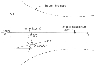
Figure 1: Impulse transmitted on an ion from a passing beam electron Sagan_91

Linearizing in the slopes of the electron trajectories, this longitudinal force can be expressed as a function of transverse force components and beam parameters Sagan_91 :

$$\Delta v_{s}=\left[-\alpha_{x}\varepsilon_{x}+(\eta\tilde{\sigma}_{\delta})(\eta^{\prime}\tilde{\sigma}_{\delta})\right]\frac{\partial\>\Delta v_{x}}{\partial x}-\alpha_{y}\varepsilon_{y}\frac{\partial\>\Delta v_{y}}{\partial y}\ .$$ (3)

The velocity changes that are produced by one bunch passage can be seen in Fig. 2. Here we used the values of Tab. 1 for top energy and Twiss parameters of $\beta_{x}=\beta_{y}=2$m, $\alpha_{x}=\alpha_{y}=1$.

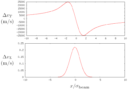
Figure 2: Transverse (top) and longitudinal (bottom) kick component in m/s vs. transverse ion position in units of the rms beam size.

In our restriction to rotationally symmetric beams, we have a dispersion of $\eta=0$, $\alpha=\alpha_{x}=\alpha_{y}$, $\varepsilon=\varepsilon_{x}=\varepsilon_{y}$, and the longitudinal kick becomes

$$\Delta v_{s}=-\alpha\varepsilon\left(\frac{\partial\>\Delta v_{x}}{\partial x}-\frac{\partial\>\Delta v_{y}}{\partial y}\right)\ .$$ (4)

For the beam parameters we studied, the longitudinal kick is typically five orders of magnitude weaker than the transverse kick, as shown in Fig. 2. In the special case of rotational symmetry, the longitudinal kick on the ion will be in the same direction for all positions. This is not true in the general case; if $\alpha_{x}$ and $\alpha_{y}$ have different signs, the kick direction can depend on the distance from the centerline Sagan_91 .

II.2 Adiabatic invariants of ion motion

In a brute force simulation, the state of each ion is characterized by its x and s position, as well as by the velocities in both directions. Every kick has to be calculated separately from the beam-beam force, which is assumed to be a function of the x and s position. Such a simulation would be very inefficient because there are two different timescales: A large number of kicks is required to resolve the sharply focused transverse ion motion, but the longitudinal motion hardly changes in a single oscillation. It is therefore not possible to simulate the motion of a realistic number of ions in this way.

The period of transverse oscillations in the beam’s potential Groebner75 ; Regenstreif76 ; Bosi82 depends on the average beam density, and for typical high-brightness beam parameters as those of Tab. 1 it is of the order of several to tens of bunch crossings. During one transverse oscillation the longitudinal position $s$ of the ion changes typically only by a fraction of a millimeter even at the largest possible ion speeds.

Ions thus oscillate in a potential that slowly changes over many periods. Because of this, an ion’s action integral over one oscillation period

$$J=m\oint v_{x}\;\mbox{d}x$$ (5)

is an adiabatic invariant of the motion. This can be used to drastically speed up the simulation.

In this improved simulation, the state of the ion is now described by its longitudinal position $s$, its longitudinal speed $v_{s}$ and its action integral $J$. For each position $s$, $J$ is a measure of the transverse oscillation amplitude $a$, because the action increases with $a$. This can most easily be seen in $(x,p_{x})$ phase space where the graph $(x(t),p_{x}(t))$ for any oscillation is a closed curve, and $J$ is the enclosed area. A closed curve that starts with a larger oscillation amplitude has to completely enclose one that starts with a smaller amplitude because different phase-space trajectories cannot cross. Solving the motion in $(J,s)$ rather than in $(x,s)$ coordinates has two advantages: (1) The degrees of freedom are reduced from 2 to 1. (2) Because $\Delta v_{s}$ changes much slower than $\Delta v_{x}$, the integration steps can be vastly increased, typically by about a factor of 10000. If the density at $s$ is to be computed, it is not enough to know the action at $s$, but one oscillation is sufficient to compute the density contribution of particles with action J.

The longitudinal acceleration averaged over one oscillation is given by the time average over individual kicks

$$\dot{v}_{s}=\langle\Delta v_{s}\rangle=-\alpha\varepsilon\;\left<\frac{\partial\>\Delta v_{x}}{\partial x}+\frac{\partial\>\Delta v_{y}}{\partial y}\right>$$

where

$$\langle\Delta v_{s}\rangle=\frac{1}{T}\;\sum_{\mbox{\tiny osc}}\Delta v_{s}\ .$$ (6)

Calculating this time average again and again for each ion is computationally demanding and wasteful. Instead, we pre-compute a table of possible values of this time average for many beam sizes $\sigma$ and amplitudes $a$ of the oscillation.

The program was further accelerated by noting that the time averaged kick as a function of $J$ can be calculated for a typical standard beam size and then rescaled for regions with other beam sizes.

To derive this scaling behavior, we use a general scaling theorem for Maxwell’s equations and the Lorentz force. If $\vec{E}(\vec{x},t)$, $\vec{B}(\vec{x},t)$, $\rho(\vec{x},t)$, and $\vec{j}(\vec{x},t)$ satisfy Maxwell’s equation, and a charged particle with mass $m$ and trajectory $\vec{r}(t)$ satisfies the Lorentz force equation, then the following scaled quantities also satisfy these equations,

$$\vec{E}_{s}(\vec{x},t) =\alpha^{2}\;\vec{E}(\alpha\vec{x},\alpha t)$$

$$\vec{B}_{s}(\vec{x},t) =\alpha^{2}\;\vec{B}(\alpha\vec{x},\alpha t)$$

$$\rho_{s}(\vec{x},t) =\alpha^{3}\rho(\alpha\vec{x},\alpha t)$$

$$\vec{j_{s}}(\vec{x},t) =\alpha^{3}\vec{j}(\alpha\vec{x},\alpha t)$$

$$\vec{r}_{s}(t) =\alpha^{-1}\vec{r}(\alpha t)$$

$$m_{s} =\alpha m\ .$$

The effect of this scaling transformation is to reduce spatial distances and time intervals by a factor $\alpha$, so that velocities remain unchanged. Also, the charge and current densities are increased by a factor $\alpha^{3}$, so that the total charge in a scaled volume remains constant.

We now want to find out how the spatial derivative of the transverse kicks changes when the transverse scale of the beam is reduced by a factor $\alpha$. If the rotationally symmetric beam produces a field $\vec{E}(x,s)$, the 3-D scaled field would be $\alpha^{2}\vec{E}(\alpha x,\alpha s)$. However, only the transverse scale changes from one beam width to another, and the longitudinal scale stays the same, signified by the unchanged line density. The charge within a 3-D scaled volume is therefore smaller by $1/\alpha$, and the field after transverse scaling is therefore $\vec{E}_{1/\alpha}(x,s)=\alpha\vec{E}(\alpha x,s)$.

The transverse scaling transformation therefore gives

$$\left(\frac{\partial\;\Delta v_{x}}{\partial x}\right)_{1/\alpha} =\left(\frac{q}{m}\right)_{\mbox{\tiny ion}}\;\frac{\partial}{\partial x}\;\int\vec{E}_{1/\alpha}(x,ct)\mbox{ d}t$$

$$=\left(\frac{q}{m}\right)_{\mbox{\tiny ion}}\;\frac{\partial}{\partial x}\;\frac{1}{c}\int\alpha\;\vec{E}(\alpha x,s)\mbox{ d}s$$

$$=\alpha^{2}\;\left(\frac{q}{m}\right)_{\mbox{\tiny ion}}\;\frac{\partial}{\partial\tilde{x}}\;\int\vec{E}(\tilde{x},ct)\mbox{ d}t$$

$$=\alpha^{2}\;\left(\frac{\partial\;\Delta v_{x}}{\partial x}\right).$$

¿From this, we see that a rescaling of the two relevant length scales $\sigma$ and $a$ has the effect

$$\frac{\partial\;\Delta v_{x}}{\partial x}\;\left(\frac{a}{\alpha},\frac{\sigma}{\alpha}\right)=\alpha^{2}\;\frac{\partial\;\Delta v_{x}}{\partial x}\;(a,\sigma)\ .$$ (7)

This is true for both derivatives, so that the time average of their sum multiplied by $\sigma^{2}$ is only a function of $a/\sigma$,

$$\sigma^{2}\;\left<\frac{\partial\>\Delta v_{x}}{\partial x}+\frac{\partial\>\Delta v_{y}}{\partial y}\right>=g(a/\sigma)\ .$$ (8)

Our goal is to express this time average as a function of the beam size $\sigma$ and the action integral $J$, so we also have to find the functional dependence of $J$ on $a$ and $\sigma$. As noted above, the electric field at a location where the beam size is reduced by a factor $\alpha$, is scaled in the transverse to $\alpha E(\alpha x,s)$. To obtain scaled transverse ion motion, we do not change the mass of the ions, i.e. $m_{s}=m$. The transverse velocity is then not changed by transverse scaling, and according to Eq. (5), the action integral is reduced by a factor $\alpha$. From this we conclude

$$J(a,\sigma)=\alpha\;J\left(\frac{a}{\alpha},\frac{\sigma}{\alpha}\right)\ .$$ (9)

Combining this result with the above analysis, we finally find

$$\left<\frac{\partial\>\Delta v_{x}}{\partial x}+\frac{\partial\>\Delta v_{y}}{\partial y}\right>=\frac{1}{\sigma^{2}}\;f(J/\sigma)\ .$$ (10)

To speed up the program, a lookup table for the function $f$ is therefore computed for a standard beam size $\sigma$ and a range of action integrals $J$. The longitudinal acceleration of the ions is then given by

$$\dot{v}_{s}=-\frac{\alpha\varepsilon}{\sigma^{2}}\;f(J/\sigma)\ .$$ (11)

II.3 Fast ion propagation to equilibrium

The toy model for our ion simulations consists of a field-free beam region of variable length $L$, so that the $\beta$-function is given by

$$\beta(s)=\beta^{*}[1+(\frac{s}{\beta^{*}})^{2}]$$ (12)

with waist at $s=0$. We then simulate the creation of ions in the beampipe through ionization processes. The ionization rate in a given volume $V$ is given by

$$\frac{\Delta N}{\Delta t\Delta V}=\rho_{e}\rho_{g}\sigma_{{\rm col}}c$$ (13)

where $\rho_{e}$ is the local particle density of the electrons as given by the Gaussian beam profile $\rho_{g}$. By integrating over the transverse directions, one obtains an equation for the number of ions created in a length $L$ of the beam

$$\frac{\Delta N}{\Delta t\Delta L}=\frac{I_{{\rm beam}}}{e}\rho_{g}\sigma_{{\rm col}}\ .$$ (14)

¿From this it is clear that ions are created with equal rate at all locations along the beam. Under the influence of the longitudinal beam force, the ions will then slowly propagate to the point with minimal potential.

In our simulation, we assume that clearing electrodes have been placed at the waist, so that ions crossing the $s=0$ line are removed. An equilibrium situation is reached when an equal number of ions are produced and removed during a given time interval. The time needed to reach this equilibrium depends on the length of the beam pipe and the steepness of the longitudinal potential. Typical values in our simulation are $10^{6}$ to $10^{8}$ bunch separations of 0.77 ns.

As a first example, we show a $L$=20m long part of the beam with a waist of $\beta^{*}=1$m at its center. The longitudinal equilibrium ion distribution for 10m up to the waist is shown in Fig. 3. There is a sharp increase in the ion density near the electrode at $s=0$m that is caused by two effects. The first is that ions which have been created at all points of the beam pass through this region and contribute to the density. The second effect is that the $\alpha$-function becomes smaller near the waist, so that ions which are created there experience a weaker longitudinal force and move more slowly to the electrode.

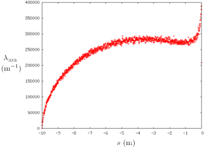
Figure 3: Longitudinal ion distribution in the steady state for the 20m beam model.

The transverse ion distribution can be characterized by its standard deviation, which is plotted in Fig. 4.

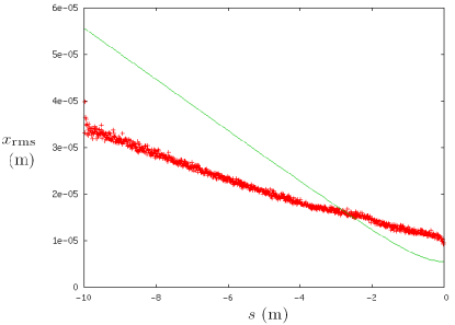
Figure 4: Beam (solid line) and ion (+) transverse standard deviations as a function of longitudinal position in the 20m beam model.

Two features of this graph can be explained easily. (a) The rms width of the ions at the start of the section (at $s=-10$m) is smaller than that of the electron beam, even though ions are created in proportion to the Gaussian electron distribution. The reason is that ions start to oscillate within the electron beam after their creation and therefore contribute to the density around zero, no matter where they were created. (b) The ion distribution contracts less than the electron beam. This can be explained by the adiabatic invariance and the scaling of the action integral. Ions that are created with an action $J$ in regions where the electron beam is wide will still have that action by the time they reach a part of the beam that is narrower by a factor $\alpha$. At that position, their oscillation amplitude will have increased relative to the beam size, because the action for a proportionally reduced oscillation amplitude would be reduced by a factor $\alpha$ according to Eq. (9).

The density profile of the transverse ion distribution at $s=\pm 1$ near the clearing electrode is shown in Fig. 5. Near the beam axis, the density diverges approximately as $1/r$, so that it is not appropriate to fit the ion distribution to a Gaussian.

For a rotationally symmetric particle density, the number of ions created in a length d$s$ and in a radius element d$r$ per time is

$$\dot{n}(r,s)\mbox{ d}r\mbox{d}s=c\sigma_{{\rm col}}\rho_{g}\rho_{e}(r,s)\;2\pi r\mbox{ d}r\mbox{d}s.$$ (15)

Subsequent to the creation of an ion at ($r_{0},s_{0}$), it travels along the beamline to $s=S(t;r_{0},s_{0})$ and oscillates through the electron beam to $R(s;r_{0},s_{0})$. Ions created between $s_{m}$ and $s$ can contribute to the distribution at $s$, and a ring element d$r$d$s$ with radius $r$ therefore contains d$n$ ions,

$$dn(r,s) = \int_{s_{m}}^{s}\int_{0}^{\infty}\int_{-\infty}^{\infty}\dot{n}(r_{0},s_{0})\mbox{ d}t\mbox{d}r_{0}\mbox{d}s_{0}$$

$$\times\delta(r-R(s;r_{0},s_{0}))\mbox{ d}r$$

$$\times\delta(s-S(t;r_{0},s_{0}))\mbox{ d}s$$

$$= \int_{s_{m}}^{s}\frac{\dot{n}(r_{0},s_{0})}{|\partial_{r_{0}}R(s;r_{0},s_{0})|}\frac{\mbox{d}s_{0}\mbox{d}r\mbox{d}s}{|\dot{S}(t;r_{0},s_{0})|}\ ,$$

where $r_{0}$ is the radius at $s_{0}$ that leads to $r$ when the ion arrives at $s$ and $t$ is the time at which it arrives, i.e. $r_{0}(s_{0};r,s)$ and $t(s_{0};r,s)$,

$$\frac{\mbox{d}n}{\mbox{d}r\mbox{d}s}(r,s) = \int_{s_{m}}^{s}\frac{\dot{n}(r_{0},s_{0})}{|\dot{S}(t;r_{0},s_{0})|}\left|\frac{\partial r_{0}}{\partial r}\right|\mbox{ d}s_{0}\ .$$ (16)

The number of particles per radius interval $\frac{{\rm d}n}{{\rm d}r{\rm d}s}(r)$ is clearly not zero for $r=0$, and the density close to zero therefore has a singularity of the form

$$\rho_{e}(r)=\frac{1}{2\pi r}\frac{\mbox{d}n}{\mbox{d}r\mbox{d}s}(0)\ .$$ (17)

Because of repulsive forces between the ions, the density at the origin cannot diverge, and we therefore estimate the radius $r_{m}$ below which these forces become larger than the forces from the electron beam. It will turn out that this radius is a very small fraction of the electron beam’s width, so that deviation from the $1/r$ density can be neglected.

We assume that the region with radius $r_{i}$ in which the ion density can be approximated as $\rho_{{\rm ion}}=\frac{A}{r}$ contains most of the charge. At some radius, the density has to fall off faster than $1/r$ to integrate to a finite value. Our assumption therefore leads to an overestimate of the ion force. Integrating $\rho_{\rm ion}$ up to $r_{i}$ leads to the ion line density $2\pi Ar_{i}=\lambda_{{\rm ion}}$.

The region that contains most of the charge has a radius $r_{i}$ that is usually smaller than the rms width of the electron beam. Only if ions were created in a very wide region of the beam, and it were to be focused down to an extremely small radius, could the ion width be much larger than the electron width. However, such extreme focusing does not occur in most beams, especially not in the Cornell ERL.

Gauss’ law within $r_{i}$ leads to the constant radial electric field

$$E_{{\rm ion}}=\frac{\lambda_{{\rm ion}}}{2\pi\epsilon_{0}r_{i}}\ .$$ (18)

The radial electric field of the electron beam has already been used in Eq. (2) and for radii much smaller than $\sigma$ simplifies to $E_{e}=\frac{\lambda r}{4\pi\epsilon_{0}\sigma^{2}}$. We can now find the radius $R$ for which the ion field is as large as the electron field, $R=\sigma\frac{\lambda_{{\rm ion}}}{\lambda}\frac{2\sigma}{r_{i}}$. As long as the number of ions per length is much smaller than the number of electrons per length, the $1/r$ scaling of the ion density is therefore correct and not altered by the ion forces in by far the largest part of the beam.

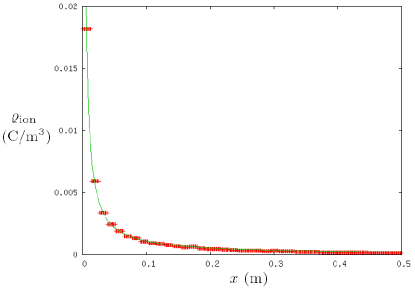
Figure 5: Ion transverse density profile at $s=\pm 1$m in the 20m beam model and comparison with a $1/r$ distribution.

III Electron motion in the ion potential

III.1 Electron propagation

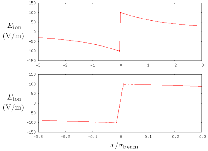
Figure 6: Electric field produced by the ions at $s=\pm 1$m in the 20m beam model.

Because of the $1/r$ ion density characteristics, the electric field of the ion distribution approaches a constant for small distances, as specified in Eq. (18). This is shown in Fig. 6. To investigate the strength of the resulting beam distortion, we simulated the propagation of a representative set of beam electrons through the ion field. Our simulation was set up to include a piece of the beampipe of length $L$, with the clearing electrode and the waist of the beam placed in the center.

The initial electron distribution is determined by random betatron amplitudes $J_{x}$ and phases $\phi_{x}$ with the density distribution

$$\rho(J_{x},\phi_{x})=\frac{1}{2\pi\varepsilon}\;e^{-J_{x}/\varepsilon}\ .$$ (19)

We also investigated the effect of the beam transversing the region of length $L$ several times, which could lead to the build-up of damaging resonances. For this study, the linear optics has to be made periodic after crossing the field-free region. This can be accomplished by including a thin half-quad with the transfer matrix

$$M_{q}=\left(\!\begin{array}[]{cc}1&0\\ -kl/2&1\end{array}\right)$$ (20)

before and after each run through the ion field. The $\alpha$-function is $\alpha_{-}=0$ before and $\alpha_{+}=\beta\;kl/2$ after the thin quadrupole. Simultaneously, this $\alpha$-function must correspond to that of a drift, i.e. $\alpha_{+}=\frac{L}{2\beta^{*}}$. Therefore,

$$kl/2=\frac{L}{2\beta\beta^{*}}=\frac{L/2}{(\beta^{*})^{2}+(L/2)^{2}}\ .$$ (21)

The simulation of the electron motion is implemented with a dynamical time step proportional to the distance from the beam axis, so that the effects of the strong field near the centerline are accounted for accurately.

As a worst case scenario, we simulated two drift regions with 200m and 100m length and a beam waist of $\beta^{*}=100$m at the center in both cases. The final phase-space distributions with and without the ion field are shown in Figs. 7 and 8.

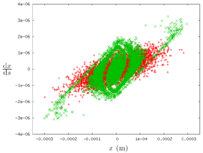
Figure 7: Electron beam phase-space distribution after transversing the 200m ion field with $\beta^{*}=100$m at its center. Dark-red $+$: phase space in a free drift, Light-green $\times$: phase space for motion through the ion field.

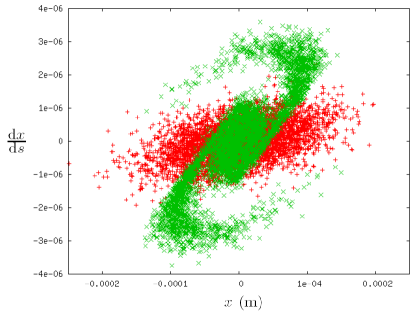
Figure 8: Electron beam phase-space distribution after transversing the 100m ion field with $\beta^{*}=100$m at its center. Dark-red $+$: phase space in a free drift, Light-green $\times$: phase space for motion through the ion field.

While passing through the ion field once, the emittance increases from 30.6pm to 53.1pm in the 100m field and to 50.7pm in the 200m field, as can be seen in Fig. 9. The electronic version of this paper contains an animation of the beam as it transverses the ion fields.

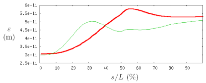
Figure 9: Emittance increase while transversing the 100 m (thick-dark-red) and 200m (thin-light-green) ion fields (horizontal axis in percent of distance $L$).

III.2 Ion-force driven emittance growth for the Cornell ERL

The previous two examples show that sections of only a few times 10 meters between clearing electrodes can produce intolerable emittance growth if the beta function is large, because in that case the beam is not very divergent and the longitudinal force that clears ions is consequently small. It therefore has to be tested whether the optics in the Cornell ERL provides fast enough ion motion to clearing electrodes, so that emittance growth is limited.

Because ions travel to the minima of the electrostatic potential, a clearing electrode has to be located at every such minimum. We therefore first calculate the potential in the beam’s center with the approximate equation Regenstreif76

$$\Phi=-\frac{I}{2\pi\epsilon_{0}c}\;\left[\frac{1}{2}+\log\frac{R\sqrt{\gamma}}{\sqrt{\varepsilon_{nx}\beta_{x}+(\eta_{x}\sigma_{\delta})^{2}}+\sqrt{\varepsilon_{ny}\beta_{y}}}\right]\ ,$$ (22)

for a round beam pipe with radius $R$ and a beam with the relativistic factor $\gamma$. This equation assumes a uniform transverse density distribution. Fig. 10 shows the relevant beam optics for the Cornell ERL and Fig. 11 shows the resulting potential in the center of the beam.

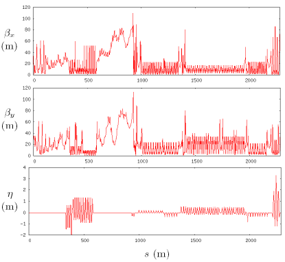
Figure 10: Beam optics for the Cornell ERL. Top to bottom: horizontal $\beta$- function, vertical $\beta$-function and horizontal dispersion.

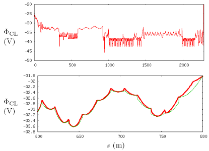
Figure 11: Top: Approximate longitudinal beam potential for the Cornell ERL. Bottom: A section of the ERL illustrating the approximation of the beam’s potential (thick-dark-red) by a round-beam model (thin-light-green).

To find a round beam approximation suitable to our simulations, we first look at the minima of this potential and calculate the $\beta$-function that would give the same potential at those locations in the case of a round beam,

$$\beta^{*}=\frac{R^{2}\gamma}{4\varepsilon_{n}\exp\left[4\Phi\pi\epsilon_{0}c/I-1\right]}\ .$$ (23)

We can then define a round beam approximation for the entire ERL lattice by using a free drift from one potential maximum to the next with $\beta(s)$ from Eq. (12). The longitudinal ion velocities near the center of the beam (where most of the ions are located) depend only on this potential gradient. As will be demonstrated by a comparison with particle tracking in Figs. 13 and 14, ions that are not in the center have the same velocity to a good approximation. This clearing speed determines the linear ion density also for non-round beams, and our round beam model should therefore be a good approximation.

The number of ions created per unit length at the longitudinal position $s_{0}$ during a time interval $t-t_{0}$ is given by

$$\frac{\mbox{d}N_{t-t_{0}}}{\mbox{d}s_{0}}=(t-t_{0})\,\left.\frac{\mbox{d}n}{\mbox{d}s\,\mbox{d}t}\right|_{s_{0}}\ ,$$ (24)

with

$$\left.\frac{\mbox{d}n}{\mbox{d}s\,\mbox{d}t}\right|_{s_{0}}=\frac{\sigma I}{e}\,\rho_{n}(s_{0})\ ,$$ (25)

where the number density of the residual gas is $\rho_{n}$, the ionization cross section is $\sigma$ and $e$ is the elementary charge. In the equilibrium state this is the same as the rate of ions per unit length originating from $s_{0}$ passing through every surface perpendicular to the beam axis, provided that the surface is located downstream from $s_{0}$.

During a time interval $t-t_{0}$, the total number of ions per unit interval from $s_{0}$ crossing the surface is given by

$$N_{s_{0}}(t)=(t-t_{0})\;\rho_{s_{0}}(s)\;v_{s_{0}}(s)\ ,$$ (26)

where $\rho_{s_{0}}(s)$ is the local linear density of ions from $s_{0}$ per unit length at the point $s$. Solving for this quantity, we obtain

$$\rho_{s_{0}}(s)=\frac{1}{v_{s_{0}}(s)}\,\left.\frac{\mbox{d}n}{\mbox{d}s\,\mbox{d}t}\right|_{s_{0}}\ ,$$ (27)

where the velocity of ions from $s_{0}$ at $s$ is given by

$$v_{s_{0}}(s)=\sqrt{\frac{2e}{m_{\mbox{\scriptsize ion}}}\left[\rule{0.0pt}{10.76385pt}V(s_{0})-V(s)\right]}\ .\rule[-12.91663pt]{0.0pt}{4.30554pt}$$ (28)

Integrating over the relevant upstream points from the nearest potential maximum to $s$ yields the total local ion density at $s$

$$\rho(s)=\int_{s_{\mbox{\tiny max}}}^{s}\rho_{s_{0}}(s)\,\mbox{d}s_{0}\ .$$ (29)

Using this method, and assuming that the residual gas density in the linac sections is reduced by a factor 100 as specified in Tab. 1, we find the linear ion densities for the Cornell ERL shown in Fig. 12.

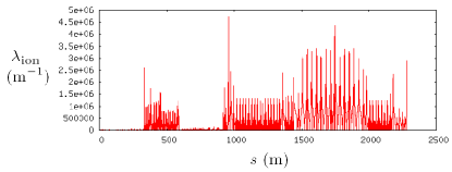
Figure 12: Estimate of the linear ion density at the Cornell ERL for a round beam approximation and clearing electrodes at the minima of the linear potential.

The two sections of the ERL with the largest linear ion densities are located at $s\approx 960$m (section A) and at $s\approx 1760$m (section B). We therefore studied these sections in detail by performing numerical ion and beam simulations. The resulting equilibrium ion densities can be found in Figs. 13 and 14. The figures demonstrate that our analytical approximation agrees well with the simulations even though the approximation assumes that all ions are in the center of the electron beam. We checked that the agreement becomes perfect in this case.

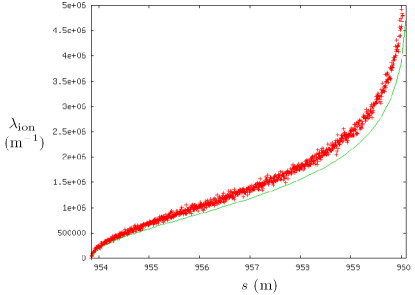
Figure 13: Simulated and analytically approximated linear ion densities near s=960m in the Cornell ERL.

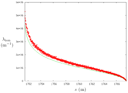
Figure 14: Simulated and analytically approximated linear ion densities near s=1760m in the Cornell ERL.

To reduce the impact of the two sections, additional clearing electrodes can be placed between the maximum and minimum of the potential. We find that by including one extra electrode, the emittance increase can be reduced from 1.04pm to 0.46pm for section A, and from 1.55pm to 0.71pm for section B.

To get a better estimate of the ion effects in the full ERL, we also simulated the ion distribution in a 34m long region around $s=1530$m, which corresponds to one of the medium high peaks in Fig. 12. Sending the beam through this section 1000 times results in the phase-space distribution in Fig. 15.

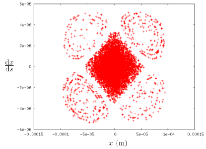
Figure 15: Electron beam phase-space plot after transversing a 34m long region with medium high ion density 1000 times.

We find that after 1000 passes through the ion field, 6.2% of the beam electrons have left the main bunch and have migrated to the four separated islands in phase space. The electronic version of this paper contains an animation of this development of the beam halo.

III.3 Outlook for non-round systems

While we have argued that our circular beam model should be quite accurate, it would be good to extend our simulations to non-round beams. However, in that case the ion propagation cannot be simulated in the same way using adiabatic invariants. Two independent invariant quantities would be needed to account for oscillations in the $x$ and $y$ directions. The problem is that the action integrals cannot be defined as the area in a phase space plane, because the ion motion is generally not a simple superposition of two independent periodic oscillations in phase-space planes. An example of such phase-space motion can be seen in Fig. 16.

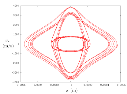
Figure 16: Example of non-periodic transverse ion motion in a non-round beam setup.

IV Conclusion

We computed the ion distribution produced by an electron beam when ion-clearing electrodes are installed. The transverse ion distributions are shown to strongly peak in the beam’s center, producing very nonlinear forces on the electron beam. These can produce strong perturbations of beam properties leading to emittance growth and halo development. These simulations rely on fast algorithms that take advantage of adiabatic invariants and scaling properties of Maxwell’s equations and the Lorentz force.

Our results are very relevant for high current Energy Recovery Linacs, where ions are produced relatively quickly, and where clearing gaps in the electron beam cannot easily be used for ion elimination. As an example we used the Cornell Energy Recovery Linac project. For simplicity we only consider the case of a circular electron beam of changing diameter. However, we parameterize this model to approximate the non-round beams of the ERL well. We found suitable places for clearing electrodes and computed the equilibrium ion density and the electron-emittance growth it would produce even after installing extra clearing electrodes at the two most dangerous places. We also showed that the nonlinear-ion forces would lead to a significant halo development.

Acknowledgments

This work has been supported by NSF cooperative agreement PHY-0202078.

References

- (1) G.H. Hoffstaetter, M.U. Liepe, Ion clearing in an ERL, NIM-A 557, p. 205 (2006)
- (2) A. Poncet, Ion trapping and clearing, Joint US-CERN School on Particle Accelerators: Benalmadena/Spain, (Nov 1992)
- (3) P. Zhou, A study of ion trapping and instability in the Fermilab antiproton accumulator, FERMILAB-THESIS-1993-40, Northwestern University (1993)
- (4) J. A. Clarke, J.A. Clarke, D.M. Dykes, S.F. Hill, E.A. Hughes, M.W. Poole, P.D. Quinn, S.L. Smith, V.P. Suller, L.A. Welbourne, Source size variation and ion effects in the SRS at Daresbury, in proceedings PAC93, Washington/DC (1993)
- (5) M. Zobov, A. Battisti, A Clozza, V. Lollo, C. Milardi, B. Spataro, A. Stella, C. Vaccarezza, Impact of ion clearing electrodes on beam dynamics in DAFNE, arXiv:0705.1223 [physics.acc-ph].
- (6) P. Zhou, P. L. Colestock and S. J. Werkema, Trapped ions and beam coherent instability, in proceedings PAC93, Washington/DC (1993)
- (7) T. O. Raubenheimer, Ion effects in future circular and linear accelerators, in proceedings PAC95 (1995)
- (8) J. Byrd, A. Chao. S. Heifets, M. Minty, T.O. Raubenheimer, J. Seeman, G. Stupakov, J. Thomson, F. Zimmermann, First observations of a “Fast Beam-Ion Instability”, Report SLAC-PUB-7507 (May 1997)
- (9) E.S. Kim, Y.J. Han, J.Y. Huang, I.S. Ko, C.D. Park, S.J. Park, H. Fukuma, H. Ikeda, Recent experiment results on fast ion instability at 2.5-GeV PLS, in proceedings PAC05, Knoxville/TN (2005)
- (10) E. V. Bulyak, The ion core density in electron storage rings with clearing electrodes, in proceedings PAC93, Washington/DC (1993)
- (11) E. V. Bulyak, Ion clearing methods for the electron storage ring, in proceedings EPAC96, Sitges/Spain (1996)
- (12) G. H. Hoffstaetter, I.V. Bazarov, S. Belomestnykh, D.H. Bilderback, M.G. Billing, J.S-H. Choi, Z. Greenwald, S.M. Gruner, Y. Li, M. Liepe, H. Padamsee, D. Sagan, C.K. Sinclair, K.W. Smolenski, C. Song, R.M. Talman, M. Tigner, Status of a plan for an ERL extension to CESR, in proceedings PAC05, Knoxville/TN (2005)
- (13) F.F. Rieke and W. Prepejchal, Ionization cross sections of gaseous atoms and molecules for high energy electrons and positrons, Phys. Rev. A, vol. 6, num. 4, p. 1507-1519 (1972)
- (14) R. Talman, AIP Conf. Proc. 153 (1987) p. 789
- (15) D. Sagan, Some aspects of the longitudinal motion of ions in electron storage rings, Nuclear Instruments and Methods in Physics Research A307 p. 171 (1991)
- (16) O. Gröbner and K. Hübner, Computation of the electrostatic beam potential in vacuum chambers of rectangular cross-section, Report CERN/ISR-TH-VA/75-27 (May 1975)
- (17) E. Regenstreif, Potential and field created by an elliptic beam inside an infinite cylindrical vacuum chamber of circular cross-section, CERN/PS/DL 77-37 (1977)
- (18) B. Bosi, Potential created by a uniform elliptical beam inside a coaxial rectangular vacuum chamber, NIM 202 p. 411 (1982)