Time-Distance Imaging of Solar Far-Side Active Regions

Abstract

It is of great importance to monitor large solar active regions in the far-side of the Sun for space weather forecast, in particular, to predict their appearance before they rotate into our view from the solar east limb. Local helioseismology techniques, including helioseismic holography and time-distance, have successfully imaged solar far-side active regions. In this Letter, we further explore the possibility of imaging and improving the image quality of solar far-side active regions by use of time-distance helioseismology. In addition to the previously used scheme with four acoustic signal skips, a five-skip scheme is also included in this newly developed technique. The combination of both four- and five-skip far-side images significantly enhances the signal-to-noise ratio in the far-side images, and reduces spurious signals. The accuracy of the far-side active region imaging is also assessed using one whole year’s solar observation.

1 INTRODUCTION

Being able to detect a large solar active region before it rotates into our view from the Sun’s far-side, and monitor a large active region after it rotates out of our view into the far-side from the Sun’s west limb, is of great importance for the space weather forecast (Schrijver & DeRosa, 2003). Using helioseismic holography technique (for a review, see Lindsey & Braun, 2000a), Lindsey & Braun (2000b) mapped the central region of the far-side Sun by utilizing double-skip solar acoustic signals visible in the near-side of the Sun but originated from or arriving into the targeted far-side area. Then, Braun & Lindsey (2001) developed furthermore this technique to map the near-limb and polar areas of the solar far-side by combining acoustic signals visible in the near-side after single and triple skips on either side of the targeted far-side area. These efforts have made monitoring active regions of the whole back side of the Sun possible, and daily solar far-side images have become available using Solar and Heliospheric Observatory/Michelson Doppler Imager (SOHO/MDI; Scherrer et al., 1995) and Global Oscillation Network Group (GONG; Harvey et al., 1996) observations. That the far-side active regions are detectable by phase-sensitive holography (Braun & Lindsey, 2000) is mainly because low- and medium-$l$ ($l$ is spherical harmonic degree) acoustic waves manifest apparent travel time deficit in solar active regions, and it is these travel time anomalies that far-side maps image, although it is still quite uncertain whether such anomalies are due to the near-surface perturbation in solar magnetic regions (Fan et al., 1995; Lindsey & Braun, 2005), or caused by faster sound speed structures in the interior of those active regions (e.g., Kosovichev et al., 2000; Zhao & Kosovichev, 2006).

Time-distance helioseismology is another local helioseismological tool that is capable of mapping the solar far-side active regions. It was demonstrated that time-distance helioseismology could map the central areas of the far-side Sun in a similar way as Lindsey & Braun (2000b) had done (Duvall et al., 2000; Duvall & Kosovichev, 2001), however, no studies have been carried out to extend the mapping area into the whole far-side. In this Letter, utilizing the time-distance helioseismology technique, I explore both the previously used four-skip scheme and a new five-skip scheme and image two whole far-side maps using four-skip and five-skip acoustic signals separately. Combining both maps gives us solar far-side images with better signal-to-noise ratio and more reliable maps of active regions on the far-side. This provides another solar far-side imaging tool in addition to the existing holography technique, hence gives a possibility to cross-check the active regions seen in both techniques, and enhances the accuracy of monitoring solar far-side active regions.

2 DATA AND TECHNIQUE

The medium-$l$ program of SOHO/MDI provides nearly continuous observations of solar oscillation modes with $l$ from $0$ to $\sim$300. The medium-$l$ data are acquired with one minute cadence and a spatial sampling of 10 arcsec (0.6 heliographic degrees per pixel) after some averaging onboard the spacecraft and ground pipeline processing (Kosovichev et al., 1997). The oscillation modes that this program observes and the continuity of such observations make the medium-$l$ data ideal to be used in solar far-side imaging.

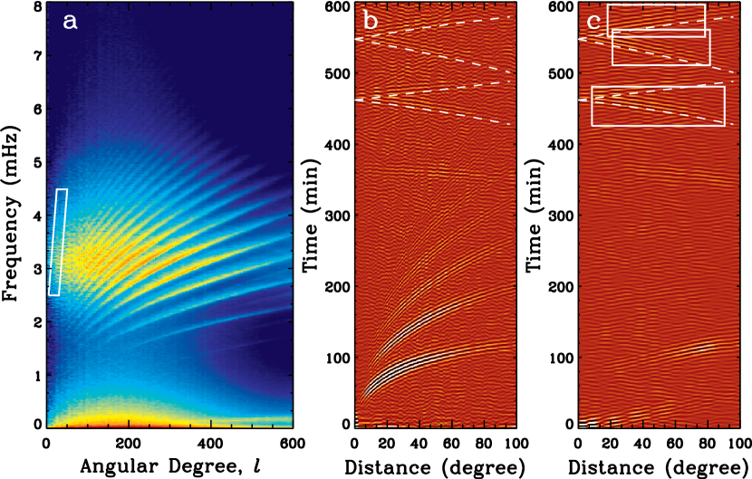
Figure 1: Power spectrum diagram ($a$) computed from a 1024-min MDI medium-$l$ data set, time-distance diagram ($b$) computed using the whole power spectrum of the same data set, and time-distance diagram ($c$) computed using only the oscillations that have frequency and $l$ included in the white quadrangle as indicated in ($a$). The white dashed lines in both ($b$) and ($c$) are theoretical time-distance relationships based on acoustic ray approximation, with the lower ‘$<$’-like curve as the fourth-skip, and the upper ‘$<$’-like curve as the fifth-skip. The lower and upper branch of each ‘$<$’-like curve represents acoustic wave propagation distance shorter and longer than $360\arcdeg$, respectively. The white boxes in ($c$) delimit the acoustic travel distances and times used for far-side imaging.

The acoustic wave signals that originate from and then return to the solar front side after traveling to the back side and experiencing four and five bounces are to be used in the time-distance far-side analysis. It is natural and often useful to first examine whether such acoustic signals are detectable by the time-distance technique. A 1024-min MDI medium-$l$ data set with a spatial size of $120\arcdeg\times 120\arcdeg$ is used for such an examination after the region is tracked with Carrington rotation rate and is remapped using Postel’s projection with the solar disk center as its remapping center. The $l-\nu$ power spectrum diagram of this data set is shown in Figure 1$a$. The time-distance diagram computed using all oscillation modes (Figure 1$b$) clearly shows acoustic bounces of up to seven times in the front side, and at the locations of the expected signals traveling back to the front side after four and five bounces, there are some not-very-clear but existing signals. Since the acoustic signals that are needed for the far-side analysis should have a fairly long single-skip travel distance, thus corresponding to low-$l$ modes, it is helpful to filter out all other acoustic modes and keep only those signals that are corresponding to the required travel distances. Such a filtering should help to improve the signal-to-noise ratio of time-distance signals at the desired distances. However, such a filtering is applied to the data after Postel’s projection, thus it only works best where the geometry is least distorted. The white quadrangle in Figure 1$a$ delimits the acoustic modes that are used in both four- and five-skip analyses (note that when computing far-side images, both four- and five-skip analyses use only part of the acoustic modes shown in the white quadrangle), covering a frequency range of $2.5-4.5$ mHz and $l$ of $3-50$, and the time-distance diagram made using only these modes (Figure 1$c$) shows clearly the four- and five-skip time-distance signals. Considering that the time-distance group travel time is a bit off from the ray approximated time, as was pointed out by Kosovichev & Duvall (1996) and Duvall et al. (1997), it is understandable that theoretical travel time is a few minutes off from the time-distance group travel time after four and five bounces.

In order to keep good signal-to-noise ratio as well as reasonable computational burden, not all acoustic signals that come back from the far-side after four or five skips are used. The white boxes in Figure 1$c$ indicate the distances that are utilized for far-side imaging. Namely, as sketched in Figure 2, for the four-skip scheme, the time-distance annulus radii are $133\fdg 8-170\fdg 0$ from the target point for the double-double skip combination that is used to map the far-side central area, and $66\fdg 9-85\fdg 0$ for the single-skip and $200\fdg 7-255\fdg 0$ for the triple-skip in the single-triple combination that is used to map the areas that are close to the far-side limb and polar regions; such a combination covers a total of $190\arcdeg$ in longitude (at the equator, $5\arcdeg$ past the limb to the front side near both limbs). For the five-skip scheme, the annulus radii are $111\fdg 6-174\fdg 0$ from the target point for the double-skip and $167\fdg 4-261\fdg 0$ for the triple-skip; this scheme covers a total of $160\arcdeg$ in longitude, less than the whole far-side. Unlike in Braun & Lindsey (2001) where far-side polar areas were also included in the imaging, to reduce unnecessary computations only areas lower than the latitude of $48\arcdeg$, where nearly all active regions are located, are included in the time-distance far-side imaging computations reported here.

The computation procedure is as follows. A 2048-min long MDI medium-$l$ data set is tracked with Carrington rotation rate, and remapped to Postel’s coordinates centered on the solar disk as observed at the mid-point of the dataset, with a spatial sampling of $0\fdg 6$ pixel^-1, covering a span of $120\arcdeg$ along the equator as well as the central meridian. This data set is then filtered in the Fourier domain to keep only the oscillation modes that have travel distances in agreement with the distances listed above. Corresponding pixels in the annuli on both sides of the target point are selected, and the cross-covariances with both positive and negative travel time lags are computed. Such computations for all distances shown in the white boxes of Figure 1$c$ are repeated. Then, both time lags are combined and all cross-covariances obtained from different distances after appropriate shifts in time that are obtained from theoretical estimates are also combined. The final cross-covariance is fitted with a Gabor wavelet function (Kosovichev & Duvall, 1996), and an acoustic phase travel time is obtained. This procedure is repeated for the double-double and single-triple combinations in the four-skip scheme, and for the double-triple combination for total distances both shorter and longer than $360\arcdeg$ in the five-skip scheme, separately. The far-side image is a display of the measured acoustic travel times after a Gaussian smoothing with FWHM of $2\fdg 0$.

3 RESULTS

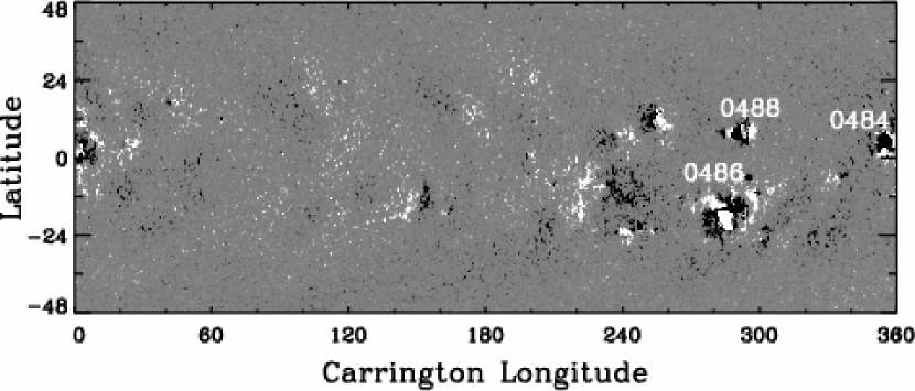
Figure 3: MDI magnetic field synoptic chart for Carrington rotation 2009, taken from October 23 to November 19, 2003, and made by use of observations near the central meridian only. Note that AR0484 is divided at the longitude of $0\arcdeg$ and $360\arcdeg$.

NOAA AR0484, AR0486 and AR0488 are selected to test this time-distance far-side imaging technique. Figure 3 shows the MDI synoptic magnetic field chart when these active regions were on the near-side of the Sun before they rotated into the far-side. AR0488 was still growing when the magnetic field data to make this synoptic map were taken.

Selected far-side images of these three active regions, obtained from separate four- and five-skip measurement schemes, and a combination of both measurements, are shown in the top three rows of Figure 4. In each image, the near-side magnetic field map is combined with the far-side acoustic travel time map, and the combined map is displayed based on Carrington longitudes. Standard deviations, $\sigma$, are 4.1 sec and 4.5 sec for four-skip and five-skip far-side maps, respectively, and after combination of both measurement schemes, $\sigma$ falls to 3.3 sec. In these maps, the three interested active regions are mostly visible in all four-skip, five-skip and combined results, except when the regions fall into the uncovered areas of five-skip measurement.

The bottom row of Figure 4 presents the same map as the third row but highlighting active regions by Gaussian smoothing the unsigned near-side magnetic field, and displaying the far-side travel time map with a threshold of $-3.5\sigma$ to $-2.0\sigma$, i.e., $-11.5$ to $-6.5$ sec. It is clear that the images combining four- and five-skip results are quite clean of spurious signals, although unidentified features still exist. It is also noteworthy that the far-side images clearly show these active regions when part of the regions were in the far-side and part in the near-side, like AR0486 and AR0488 in the fourth row and third column of Figure 4.

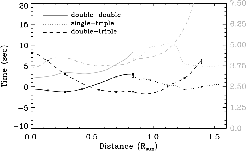
Figure 5: Background travel time variations (black curves) and travel time rms variations (grey curves) as functions of angular distance from the antipode of solar disk center for different combinations of acoustic wave bounces. Scales for grey curves are marked on the right hand side of the figure.

Both four- and five-skip far-side acoustic travel times are displayed after a mean travel time background is removed. It turns out that the background mean travel time depends on its angular distance from the antipode of the solar disk center. Figure 5 presents the variation of background mean travel times at different locations for both measurement schemes after the mean value of the background is removed. Basically, the mean acoustic travel times vary with a magnitude of $\sim$4 sec for four-skip measurement, and a magnitude of $\sim$9 sec for five-skip measurement. The measured mean acoustic travel times are shorter for the four-skip scheme, but longer for the five-skip scheme when the targeted areas are near the limb and near the antipode of the solar disk center. These variations are unlikely physical, yet it is unclear why there are such variations in the measurement. The rms of travel times can be used to assess the quality of far-side images. Also shown in Figure 5 is travel time rms variation with distance to the far-side center. It shows that double-double scheme has the lowest rms near the far-side center, while the single-triple scheme has the lowest rms near the far-side limb. For the five-skip measurement, it has the lowest rms when at and roughly $30\arcdeg$ from the far-side center, and the rms increases substantially close to the limb.

It is interesting to make a statistical study investigating how accurate the far-side active region imaging is. Since sometimes active regions change fast, grow or decay unexpectedly, it is quite impossible to make a precise assessment on the accuracy of far-side imaging. Therefore, the results given below can only be regarded as a reference. The far-side images of the whole year of 2001 were computed at 12-hour intervals, and a total of 730 images were obtained and displayed in the same way as the bottom row of Figure 4. Typically, a solar area is located on the far-side of the Sun for about 13.5 days, or 27 far-side images. Far-side images are often noisy, and even for a large active region, it is quite unlikely for it to be unambiguously visible in each of 27 images. Also, active regions on the far-side grow and decay as well. For these reasons, if an area is visible as dark in our figures 6 times (or on 3 days) on the other side, where 6 is an arbitrary number, that area is regarded as an active region. Based on this assumption, it is found that for 59 active regions that rotate into the near-side from the east limb, 53 (or $89.8\%$) are able to be detected far-side, and for 63 active regions that rotate into the far-side from the west limb, 56 (or $89.0\%$) are detectable on the far-side. Among these regions, 33 are actually detected both before and after the near-side appearance. And, from the other perspective, for 61 regions that are detected by far-side imaging rotating into the far-side from the west limb, 55 (or $90.1\%$) are visible near the west limb of the near-side; for 53 active regions that are detected by far-side imaging rotating out of the far-side into the near-side, 49 (or $92.4\%$) are visible near the east limb of the near-side. Among these regions, 28 are visible on the near-side before and after the region is located in the far-side. These statistics do not count all active regions that appeared in that year, but only those that have a diameter roughly larger than $8\fdg 0$ after projected into a spatial resolution of solar disk center and viewed in a figure like the fourth row of Figure 4, when these regions are near either limb of of the Sun.

4 DISCUSSION

By combining four-skip and five-skip measurement schemes, I have successfully made time-distance far-side images of the Sun with a fast computation speed. The combination significantly enhances the signal-to-noise ratio of far-side acoustic travel times over either four- or five-skip measurement, thus making the composite far-side active region map much cleaner. It helps to remove most, but not all of the spurious features that signify active regions. On the other hand, the combination of both maps also remove some small active regions that can otherwise be seen in one map or the other.

Time-distance far-side imaging provides another whole far-side imaging tool in addition to the existing helioseismic holography technique. It gives results that are in reasonable agreement with the holography results, which can be seen at SOHO/MDI website, by visual comparison, yet detailed comparisons are not done. It is intriguing to calibrate the measured far-side acoustic travel times into magnetic field strength, and some efforts have been taken using holography results (González Hernández et al., 2007). However, there are some apparent difficulties to carry out the calibration, because the far-side images of active regions are often relatively noisy, and sizes and shapes of those regions change from image to image. In addition, the magnetic field strengths of the far-side active regions are also unknown, although the full sphere magnetic field made by use of flux dispersal model (Schrijver & DeRosa, 2003) may help in this. Perhaps eventually, a numerical simulation of solar oscillations in the whole Sun is needed to determine a satisfactory calibration.

It is notable that the five-skip measurement scheme has a large fraction of overlapping areas as the four-skip measurement in the annulus of one side, and has one more skip on the other side (see Figure 2), but results from both measurement schemes have quite uncorrelated noises (see Figure 4). It is unlikely that the noise differences of two schemes are caused while waves travel merely one more skip, $1/5$ of the total distance, however, it may imply noises come from data or the filtering of geometrically distorted data.

The holography far-side images show strong acoustic travel time variation from the far-side center to limb, with an order of 70 sec or so in their four-skip measurement scheme (P. Scherrer, private communication), and this is believed (C. Lindsey, private communication) to be connected with the “ghost signature” described by Lindsey & Braun (2004). Although such a travel time variation trend also exists in time-distance far-side images, the variation magnitude is merely 4 sec in four-skip scheme, substantially smaller than the holography trend. The variation in the five-skip scheme measurement is about twice of that in the four-skip scheme. What causes such travel time variations in our measurement, though small, is worth further investigation.

With the availability of both time-distance and helioseismic holography far-side images, it is more robust to monitor activities on the far-side of the Sun, and we can forecast the appearance of large active regions rotating into our view from the far-side with more confidence. Furthermore, the success in far-side imaging provides us some experiences and confidence in analyzing low- and medium-$l$ mode oscillations by use of local helioseismology techniques, and this will greatly help us in analyzing solar deeper interiors and polar areas by use of these techniques.

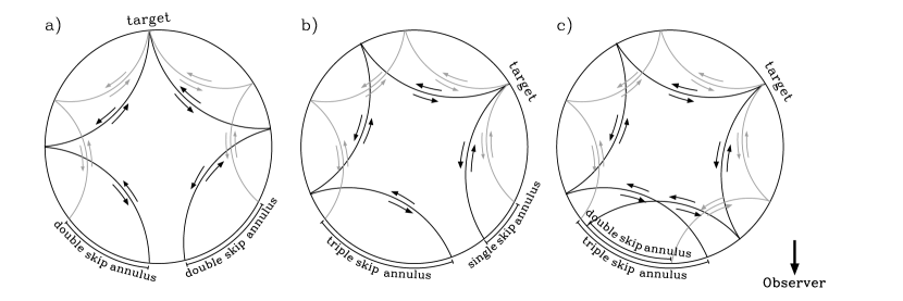
Figure 2: Sketches for four-skip measurement schemes, which includes ($a$) double-double skip combination when the target point is near the central area of the far-side and two sets of double-skip rays are located on both sides of the target point, and ($b$) single-triple skip combination when the target point is near the limb or polar area of the far-side and one set of single-skip and one set of triple-skip rays are located on either side of the target; and, five-skip measurement schemes ($c$) when one set of double-skip and one set of triple-skip rays are located on the either side of the target point.

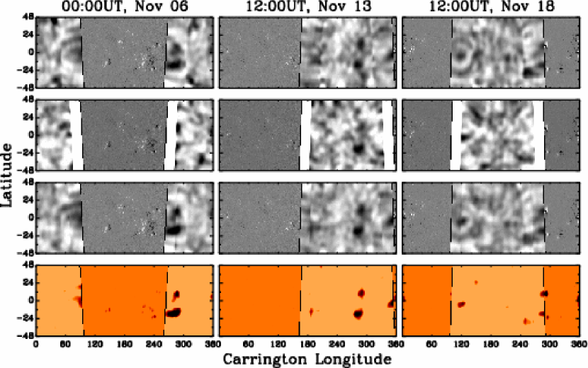
Figure 4: Results of time-distance far-side active region imaging, obtained from four-skip (first row), five-skip (second row), and combination of four- and five-skip measurements (third and bottom row). From the left to the right column, images were obtained at 00:00UT of November 6, 12:00UT of November 13, and 12:00UT of November 18, 2003, respectively. The given observation time for far-side image is the middle time of its 2048-min observational period. Each black and white image displays a combination of the near-side MDI magnetic field map and a time-distance far-side acoustic travel time map. The boundaries between the far-side and near-side are not vertical because of the solar B-angle adjustment. Magnetic field is displayed with a range of $-150$ to 150 Gs, and the acoustic travel time ranging from $-12$ to 12 sec. Blank regions in five-skip images indicate areas that cannot be covered by this measurement. Color images display the near-side map with a range of 40 to 150 Gs after a Gaussian smoothing of unsigned magnetic field with a same FWHM that is applied to travel time maps, and display the far-side map with a range of $-3.5\sigma$ to $-2.0\sigma$ in order to highlight the far-side active regions that are of our interest. To better distinguish far-side and near-side images, different color contrast is used.

References

- Braun & Lindsey (2000) Braun, D. C., & Lindsey, C. 2000, Sol. Phys., 192, 307
- Braun & Lindsey (2001) Braun, D. C., & Lindsey, C. 2001, ApJ, 560, L189
- Duvall & Kosovichev (2001) Duvall, T. L., Jr., & Kosovichev, A. G. 2001, in IAU Symp. 203, Recent Insights into the Physics of the Sun and Heliosphere: Highlights from SOHO and Other Space Missions, ed. P. Brekke, B. Fleck, & J. B. Gurman (San Francisco: ASP), 159
- Duvall et al. (2000) Duvall, T. L., Jr., Kosovichev, A. G., & Scherrer, P. H. 2000, Bull. Am. Astr. Soc. 32, 837
- Duvall et al. (1997) Duvall, T. L., Jr., et al. 1997, Sol. Phys., 170, 63
- Fan et al. (1995) Fan, Y., Braun, D. C., & Chou, D.-Y. 1995, ApJ, 451, 877
- González Hernández et al. (2007) González Hernández, I., Hill, F., & Lindsey, C. 2007, ApJ, submitted
- Harvey et al. (1996) Harvey, J. W., et al. 1996, Science, 272, 1284
- Kosovichev & Duvall (1996) Kosovichev, A. G., & Duvall, T. L., Jr. 1996, in Proceedings of SCORe’96 Workshop: Solar Convection and Oscillations and Their Relationship, ed. F. P. Pijpers, J. Christensen-Dalsgaard & C. S. Rosenthal (Dordrecht: Kluwer), 241
- Kosovichev et al. (2000) Kosovichev, A. G., Duvall, T. L., Jr., & Scherrer, P. H. 2000, Sol. Phys., 192, 159
- Kosovichev et al. (1997) Kosovichev, A. G., et al. 1997, Sol. Phys., 170, 43
- Lindsey & Braun (2000b) Lindsey, C., & Braun, D. C. 2000b, Science, 287, 1799
- Lindsey & Braun (2000a) Lindsey, C., & Braun, D. C. 2000a, Sol. Phys., 192, 261
- Lindsey & Braun (2004) Lindsey, C., & Braun, D. C. 2004, ApJS, 155, 209
- Lindsey & Braun (2005) Lindsey, C., & Braun, D. C. 2005, ApJ, 620, 1107
- Scherrer et al. (1995) Scherrer, P. H., et al. 1995, Sol. Phys., 162, 129
- Schrijver & DeRosa (2003) Schrijver, C. J., & DeRosa, M. L. 2003, Sol. Phys., 212, 165
- Zhao & Kosovichev (2006) Zhao, J., & Kosovichev, A. G. 2006, ApJ, 643, 1317