Anisotropic small-scale constraints on energy in rotating stratified turbulence

Abstract

Rapidly rotating, stably stratified three-dimensional inviscid flows conserve both energy and potential enstrophy. We show that in such flows, the forward cascade of potential enstrophy imposes anisotropic constraints on the wavenumber distribution of kinetic and potential energy. The horizontal kinetic energy is suppressed in the large, nearly horizontal wave modes, and should decay with the horizontal wavenumber as $k_{h}^{-3}$. The potential energy is suppressed in the large, nearly vertical wave modes, and should decay with the vertical wavenumber as $k_{z}^{-3}$. These results augment the only other exact prediction for the scaling of energy spectra due to constraints by potential enstrophy obtained by Charney (J. Atmos. Sci. 28, 1087 (1971)), who showed that in the quasi-geostrophic approximation for rotating stratified flows, the energy spectra must scale isotropically with total wavenumber as $k^{-3}$. We test our predicted scaling estimates using resolved numerical simulations of the Boussinesq equations in the relevant parameter regimes, and find reasonable agreement.

Classical quasi-geostrophic (QG) flow is a useful approximation for rapidly rotating, strongly stratified flows Pedlosky (1986); Salmon (1998). In this approximation, the zeroth-order expansion of the velocity in the rotation and stratification parameters is geostrophic, meaning that the Coriolis force is balanced by the pressure gradient force. Furthermore the linear plane-waves called inertia-gravity waves are eliminated to the lowest order. This leads to a simplification of the dynamics which is described entirely by the evolution of potential vorticity $q_{qg}$ Charney (1971):

$$\frac{\partial q_{qg}}{\partial t} + {\bm{u}_{0}}_{h}\cdot\nabla q_{qg}=0,$$ (1)

$$\mbox{where}\quad q_{qg} = f\frac{\partial\theta}{\partial z}-N{\omega}_{3},$$ (2)

where ${\bm{u}_{0}}_{h}$ is the leading order (horizontal) geostrophically balanced velocity, $\theta$ is the density fluctuation scaled to have the same dimensions as velocity, $\omega_{3}=(\nabla_{h}\times{\bm{u}}_{h})\cdot\hat{\bm{z}}$ is the $z$-component of the vorticity, $f$ and $N$ are the Coriolis and Brunt-Väisälä (buoyancy) frequencies respectively of a system which is rotating stratified in the $z$-direction. In QG flow, the vertical velocity $\bm{w}$ appears as a correction to leading order geostrophic balance.

In 1971, Charney Charney (1971) showed that the global conservation of total energy $E_{T}=\frac{1}{2}\int(|\bm{u}|^{2}+\theta^{2})d\bm{x}$, and potential enstrophy $Q_{qg}=\frac{1}{2}\int|q_{qg}|^{2}d\bm{x}$ by inviscid three-dimensional (3d) QG flow is analogous to conservation of energy and enstrophy in non-rotating two-dimensional turbulence (see for example Tung and Welch (2001) for further discussion on the assumptions and details of Charney’s work). Following the classical theory of 2d turbulence Fjortoft (1953); Kraichnan (1967), Charney predicted an inverse (upscale) cascade of energy with corresponding large-scale energy spectrum $E_{T}(k)\propto\varepsilon^{2/3}k^{-5/3}$, and a forward (downscale) cascade of potential enstrophy with corresponding small-scale energy spectrum $E_{T}(k)\propto\varepsilon_{Q}^{2/3}k^{-3}$, where $k$ is the wavenumber and $\varepsilon$ and $\varepsilon_{Q}$ are the transfer rates of energy and potential enstrophy, respectively.

In theory, as the rotation and stratification of a 3d fluid become infinitely strong, the inertia-gravity waves are eliminated to lowest order, giving leading order QG flow satisfying (1,2). In practice, for very large but finite rotation and stratification, the inertia-gravity waves strongly influence the small-scale dynamics leading to $E_{T}(k)\sim k^{-\gamma}$ where $1<\gamma<2$ Bartello (1995); Babin et al. (1997) in the high wavenumbers. The underlying leading order QG scaling of $k^{-3}$ predicted by Charney can then only be extracted by separating the QG (or geostrophic) modes from the wave (or ageostrophic) modes by either suitably projecting the full solutions onto the QG modes Bartello (1995); Smith and Waleffe (2002) or by filtering out the ageostrophic inertia-gravity waves Salmon (1998).

In the present work we consider rotating stratified turbulence retaining both the leading order QG as well as all sub-leading contributions from inertia-gravity waves and other nonlinear waves. We show that in this parameter regime, as in classical QG, potential enstrophy plays a significant role in constraining the energy. For a wavevector $\bm{k}=k_{x}\hat{\bm{x}}+k_{y}\hat{\bm{y}}+k_{z}\hat{\bm{z}}$ the horizontal component is $k_{h}=(k_{x}^{2}+k_{y}^{2})^{1/2}$ and the vertical component is $k_{z}$. We show that the potential enstrophy dominates over potential energy in the large, nearly vertical modes ($k_{z}/k_{h}\gg 1$), resulting in a potential energy spectrum scaling of $k_{z}^{-3}$ for large $k_{z}$. And potential enstrophy also dominates over horizontal kinetic energy in the large, nearly horizontal modes ($k_{h}/k_{z}\gg 1$), resulting in a horizontal kinetic energy spectrum scaling of $k_{h}^{-3}$ for large $k_{h}$. These are the first scaling estimates for the spectra of rapidly rotating and stably stratified flows away from pure QG, obtained solely using the relationship between potential enstrophy and energy as a function of scale. Such scaling laws, apart from being benchmarks, are potentially useful in parameterizing the turbulent small scales in large simulations of rotating stratified flows thus reducing the computational expense of explicitly resolving the small scales.

We begin with the Boussinesq equations for rotating, stably stratified and incompressible flow given by Embid and Majda (1998):

$$\frac{D}{Dt}\bm{u}+f\hat{\bm{z}}\times\bm{u}+\nabla p+N\theta\hat{\bm{z}} = \nu\nabla^{2}\bm{u}+{\cal F}$$

$$\frac{D}{Dt}\theta-Nw = \kappa\nabla^{2}\theta$$ (3)

$$\nabla\cdot\bm{u} = 0,$$

where $\displaystyle\frac{D}{Dt}=\frac{\partial}{\partial t}+\bm{u}\cdot\nabla$, $\bm{u}$ is the velocity, $w$ is its vertical component, $p$ is the effective pressure and $\cal F$ is an external input or force. The total density is ${\cal\rho}_{T}(\bm{x})=\rho_{0}-bz+\rho(\bm{x})$, where $\rho_{0}$ is the constant background, $b$ is also constant and larger than zero for stable stratification in the vertical $z$-coordinate, $\rho$ is the density fluctuation such that $|\rho|\ll|bz|\ll\rho_{0}$ and $\displaystyle\theta=\rho({g}/{b\rho_{0}})^{1/2}$ has the dimensions of velocity. The Coriolis parameter $f=2\Omega$ where $\Omega$ is the constant rotation rate about the $z$-axis, the Brunt-Väisälä frequency $\displaystyle N=({gb}/{\rho_{0}})^{1/2}$, $\nu=\mu/\rho_{0}$ is the kinematic viscosity and $\kappa$ is the mass diffusivity coefficient. We assume periodic or infinite boundary conditions. The relevant non-dimensional parameters for this system are the Rossby number $Ro=f_{nl}/{f}$ and the Froude number $Fr=f_{nl}/{N}$, where $f_{nl}=(\epsilon_{f}k_{f}^{2})^{1/3}$ is the non-linear frequency given input rate of energy $\epsilon_{f}$ Smith and Waleffe (2002). Thus $Ro$ and $Fr$ are the ratios of rotation and stratification timescales respectively to the nonlinear timescale.

The Boussinesq equations conserve the following quantities for ${\cal F}=\nu=\kappa=0$,

$$\mbox{total energy}~{}E_{T}=E+P,~{}~{}\frac{D}{Dt}\int E_{T}~{}d\bm{x} = 0,$$

$$\mbox{potential vorticity}~{}q=\Big{(}\bm{\omega}_{a}\cdot\nabla\rho_{T}\Big{)},~{}~{}\frac{Dq}{Dt} = 0,$$

$$\mbox{potential enstrophy}~{}Q=\frac{1}{2}q^{2},~{}~{}\frac{DQ}{Dt}=\frac{D}{Dt}\int Q~{}d\bm{x} = 0.$$

$E=\frac{1}{2}|\bm{u}|^{2}$ is the kinetic energy, $P=\frac{1}{2}\theta^{2}$ is the potential energy of the density fluctuations. The absolute vorticity $\bm{\omega}_{a}=\bm{\omega}+f\hat{\bm{z}}$ and the relative (or local) vorticity $\bm{\omega}=\nabla\times\bm{u}$. Potential vorticity may be written in terms of $\theta$ as

$$q=fN+\bm{\omega}\cdot\nabla\theta+f\frac{\partial\theta}{\partial z}-N\omega_{3}.$$ (4)

The constant part $fN$ does not participate in the dynamics and we will therefore neglect it from now on. The linear part of (4) is precisely $q_{qg}$ of (2). In what follows we will assume that $\nu\rightarrow 0$ and $\kappa\rightarrow 0$ such that Prandtl number $Pr=\nu/\kappa=1$, and the force $\cal{F}$ is confined to the lowest modes. Thus we assume a conventional ‘inertial-range’ of turbulent scales wherein the transfer of conserved quantities dominates over both their dissipation and forcing.

As $Ro\rightarrow 0$ and $Fr\rightarrow 0$, the potential vorticity $q$ approaches $q_{qg}$ Bartello (1995); Kurien et al. (2006). This is easily observed by considering the non-dimensional form of (4) namely $q=\bm{\omega}\cdot\nabla\theta+Ro^{-1}\frac{\partial\theta}{\partial z}-Fr^{-1}\omega_{3}$, and letting $Ro$ and $Fr$ tend to zero together. In fourier representation:

$$\tilde{q}(\bm{k})\simeq fk_{z}\tilde{\theta}+iN\bm{k}_{h}\times\tilde{\bm{u}}_{h}=fk_{z}\tilde{\theta}+iNk_{h}\tilde{u}_{h}$$ (5)

where $\tilde{\cdot}$ denotes fourier coefficients, the total wavevector $\bm{k}$ = $\bm{k}_{h}+k_{z}\hat{\bm{z}}$, the horizontal wavevector component has length $k_{h}=({k_{x}^{2}+k_{y}^{2}})^{1/2}$, the vertical wavenumber is $k_{z}$ and $\bm{u}_{h}$ is the horizontal velocity vector with magnitude $u_{h}=(u_{x}^{2}+u_{y}^{2})^{1/2}$. We assume that the vertical velocity $w=u_{z}\sim 0$ in the lowest order (classical QG) thus obtaining the last equality of Eq. (5).

We take both $N$ and $f$ to be very large, and $N/f=1$ so that $Ro=Fr$. This approaches the special case $Ro\rightarrow 0$ and $Fr\rightarrow 0$ while $Ro=Fr$ which was shown rigorously to be leading order QG in Embid and Majda (1998). For $k>k_{f}$, scales smaller than the forcing scale, we consider two cases:

1) Case $\displaystyle\frac{k_{z}}{k_{h}}\gg 1$ . These are the more vertical wavenumber modes corresponding loosely to flat ‘pancake’ scales in physical space. Eq. (5) reduces to $\tilde{q}\simeq fk_{z}\tilde{\theta}$, yielding the following relation between potential enstrophy and potential energy distribution in spectral space,

$$Q(k_{h},k_{z})=\frac{1}{2}|\tilde{q}|^{2}=f^{2}k_{z}^{2}P(k_{h},k_{z}),$$

which upon integration over some high vertical wavenumber interval leads to the following constraint:

$$\int_{\kappa_{z}}^{\infty}Q(k_{h},k_{z})dk_{z}\gg f^{2}\kappa_{z}^{2}\int_{\kappa_{z}}^{\infty}P(k_{h},k_{z})~{}dk_{z},$$

where the potential energy spectrum $P(k_{h},k_{z})=\frac{1}{2}|\tilde{\theta}|^{2}$. Thus, for sufficiently high wavenumbers $\kappa_{z}\rightarrow\infty$, the potential enstrophy $Q$ forms the dominant forward cascade and, in order to remain finite, suppresses the potential energy $P$ in this regime. The dimensional argument following Fjortoft (1953); Kraichnan (1967) assumes that in this wavenumber limit, the potential energy spectrum must depend on the potential enstrophy flux rate $\varepsilon_{Q}$ and the vertical wavenumber $k_{z}$, so that:

$$P(k_{h},k_{z})\sim\varepsilon_{Q}^{2/5}k_{z}^{-3}.$$ (6)

2) Case $\displaystyle\frac{k_{h}}{k_{z}}\gg 1$ . These are the wide flat wavenumber modes corresponding to the tall columnar scales in physical space. In this limit Eq. (5) reduces to $\tilde{q}=iNk_{h}\tilde{u}_{h}$. Following the same arguments as for potential energy above, we obtain that the potential enstrophy dominates the forward cascade in the regime $k_{h}/k_{z}\gg 1$, resulting in suppression of horizontal kinetic energy resulting in the following scaling estimate:

$$E_{h}(k_{h},k_{z})\sim\varepsilon_{Q}^{2/5}k_{h}^{-3}.$$ (7)

where the horizontal kinetic energy $E_{h}(k_{h},k_{z})=\frac{1}{2}|\tilde{u}_{h}|^{2}$.

Our new scaling predictions (6) and (7) describe the spectral statistics of the full flow for small but finite $Ro$ and $Fr$, not just the leading order QG part of the dynamics. The main purpose of this paper is to show that the potential enstrophy imposes predictable constraints on the energy in rapidly rotating stratified flow even when the flow is not strictly QG. In the next sections we seeking to numerically verify our predictions for the energy spectra in the two limiting regimes in wavenumber.

We simulate the Boussinesq equations (3) taking $N=f$ very large. We use a pseudo-spectral code in a periodic cube of side $L=1$, generating wavenumbers which are integer multiples of $2\pi$. A fourth-order Runge-Kutta time integration is used and the inertia-gravity wave frequencies are resolved in our explicit scheme. Since we are interested in the small scales (high wavenumbers), we use a low-wavenumber stochastic forcing centered at $k_{f}=4$. In order to extend the inertial range in the high wavenumbers, the viscous dissipation is modeled using a hyperviscous term $(-1)^{p+1}\nu(\nabla^{2})^{p}\bm{u}$, where $p=8$ in place of the normal laplacian viscosity term $\nu\nabla^{2}\bm{u}$. The hyperviscosity coefficient $\nu$ is dynamically chosen based on the energy in the highest mode for both momentum and mass diffusion following Smith and Waleffe (2002), $\nu(t)=2.5\Big{(}\frac{E(k_{m},t)}{k_{m}}\Big{)}^{1/2}k_{m}^{2-2p}$ where $k_{m}$ is the highest available wavenumber and $E(k_{m},t)$ is the kinetic energy in that wavenumber. An analogous scheme is used for the diffusion term in Eq. (3) for the evolution of $\theta$. The parameters of a few of our runs are given in Table 1. We report the results from data $\#4$ for which $Ro$ and $Fr$ are the smallest and the resolution is the best.

#	$n$	$k_{f}$	$N/f$	$Ro$	$Fr$	$\epsilon_{f}$
1	256	4	1	0.029	0.029	0.62
2	256	4	1	0.014	0.014	0.61
3	256	4	1	0.0072	0.0072	0.60
4	512	4	1	0.0072	0.0072	0.60

Table 1: Parameters of Boussinesq calculations: $n$ – number of grid points to a side; $k_{f}$ – forcing wavenumber; $N$ – Brunt-Väisälä frequency, $Ro$ – Rossby number; $Fr$ – Froude number; $\epsilon_{f}$ – rate of input of kinetic energy.

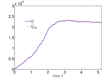
Figure 1: Total potential enstrophy $Q$ and its linear part $Q_{qg}$ for data #4. The two are indistinguishable, indicating purely quadratic potential enstrophy. Time $t$ is in dimensional units.

Figure 1 shows the evolution of the total potential enstrophy $Q$ from (4), and its linear, quasi-geostrophic piece $Q_{qg}$. The former is indistinguishable from the latter indicating that the nonlinear part of the potential vorticity $\bm{\omega}\cdot\nabla\theta$ is negligible and thus the potential enstrophy is quadratic. The system is QG in the leading order, or near-QG in the sense described above. The mean potential enstrophy has reached a nearly steady value in the time range $2.5<t<5.2$, which corresponds to between 5 and 11 non-linear time cycles, or 5000 to 10400 rotation (stratification) cycles.

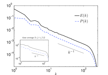
Figure 2: Log-log plot of spherical shell averaged potential and kinetic energy spectra for data $\#4$ at time $t=5.2$. The high wavenumber scaling is $k^{-1}$ indicating that in this representation the energy is dominated by waves. Inset: Same spectra averaged over time $3\leq t\leq 5.2$.

Figure 2 shows the shell-averaged kinetic and potential energy spectra for our simulation, computed as follows:

$$E(k)=\frac{1}{2}\sum_{k^{\prime}}|\tilde{\bm{u}}(\bm{k}^{\prime})|^{2},~{}~{}P(k)=\frac{1}{2}\sum_{k^{\prime}}|\tilde{\theta}(\bm{k}^{\prime})|^{2}$$

where $k-0.5\leq k^{\prime}<k+0.5$ thus including all wavenumbers in the spherical shell of average radius $k$. The scaling of both $E(k)$ and $P(k)$ is $k^{-1}$ for $k\gg k_{f}$ which indicates that by this measure the high wavenumbers are still dominated by waves Bartello (1995); Sukhatme and Smith (2007). The inset shows the average of the spectra over the time period $3\leq t\leq 5.2$ over which the potential enstrophy is constant as seen in Fig. 1. The time-averaged spectra also show a scaling very close to $k^{-1}$ indicating that the small scales ($k>k_{f}$) have achieved close to a statistically steady state.

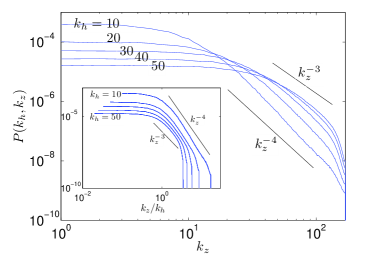
Figure 3: Log-log plot of potential energy density $P(k_{h},k_{z})$ vs. $k_{z}$ for data $\#4$ averaged over time $3\leq t\leq 5.2$. Each curve is the spectrum for a different fixed value of $k_{h}$. For $10\leq k_{h}\leq 50$ and $k_{z}\gg k_{f}$, the scaling ranges between $k_{z}^{-4}$ and $k_{z}^{-3}$. Inset: Same spectra versus $k_{z}/k_{h}$ shows that the ‘turnover’ to the inertial range scaling for all the curves emerges only when $k_{z}/k_{h}\geq 1$.

The potential energy and horizontal kinetic energy spectra as functions of $k_{h}$ and $k_{z}$ were computed as double sums according to:

$$P(k_{h},k_{z})=\frac{1}{2}\sum_{k_{h}^{\prime},k_{z}^{\prime}}|\tilde{\theta}(\bm{k}^{\prime})|^{2},~{}~{}E_{h}(k_{h},k_{z})=\frac{1}{2}\sum_{k_{h}^{\prime},k_{z}^{\prime}}|\tilde{\bm{u}}_{h}(\bm{k}^{\prime})|^{2}$$

where $k_{z}[k_{h}]-0.5\leq k_{z}^{\prime}[k_{h}^{\prime}]<k_{z}[k_{h}]+0.5$. Figure 3 shows $P(k_{h},k_{z})$ as a function of $k_{z}$ for various values of $k_{h}$. For $10\leq k_{h}\leq 50$ and $k_{f}\leq k_{z}\leq 100$, the scaling for $P(k_{h},k_{z})$ ranges between $k_{z}^{-4}$ and $k_{z}^{-3}$ indicating stronger suppression of potential energy than the dimensional prediction of Eq. (6). As $k_{h}$ increases $P(k_{h},k_{z})$ also persists more strongly into the high $k_{z}$. Conversely, for a fixed small $k_{z}\leq k_{f}$, the smaller $k_{h}$ spectra have more energy, indicative of a growth of potential energy as $k_{z}\ll k_{f}$ for small $k_{h}$. The inset of Fig. 3 shows the same spectra versus $k_{z}/k_{h}$ which shows clearly that the inertial range scaling for each $k_{h}$ emerges only when $k_{z}/k_{h}\geq 1$, the predicted range for Eq. (6). Overall the constraints on potential energy due to potential enstrophy are thus highly anisotropic in scale and consistent with our prediction.

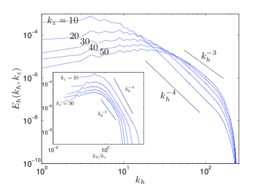
Figure 4: Log-log plot of horizontal kinetic energy density $E_{h}(k_{h},k_{z})$ vs. $k_{h}$ for data $\#4$ averaged over time $3\leq t\leq 5.2$. Each curve is a different value of $k_{z}$. For $10\leq k_{z}\leq 50$ there the scaling ranges between $k^{-4}$ and $k^{-3}$. Inset: Same spectra vs. $k_{h}/k_{z}$ showing that the inertial range emerges as $k_{h}/k_{z}\geq 1$ as predicted.

Figure 4 shows $E_{h}{k_{h},k_{z}}$ as a function of $k_{h}$ for various values of $k_{z}$. For $10\leq k_{z}\leq 50$ and $10<k_{h}<100$, the horizontal energy spectrum $E_{h}(k_{h},k_{z})$ scales between $k_{h}^{-4}$ and $k_{h}^{-3}$ consistent with the suppression of horizontal kinetic energy by potential enstrophy in these modes. As $k_{h}$ grows, the horizontal kinetic energy persists more strongly into the high $k_{h}$. Conversely, for a fixed small $k_{h}$, the smaller $k_{z}$ have more energy, indicating a growth of energy upscale in $k_{z}$. The inset of Fig. 4 shows again that the inertial range scaling predicted arises only in the anisotropic regime $k_{h}/k_{z}\geq 1$ consistent with prediction.

In conclusion, we have deduced separate scaling laws for horizontal kinetic and potential energy spectra, both of which are constrained in the small scales by potential enstrophy in rapidly rotating stably stratified flows. Potential enstrophy suppresses the potential energy in the large, nearly vertical modes, and also suppresses horizontal kinetic energy in the large, nearly horizontal modes; the resulting energy densities in these modes scales as $k_{z}^{-3}$ and $k_{h}^{-3}$ respectively. Our test simulations data show even steeper scaling of the spectra than predicted (greater suppression due to potential enstrophy). The numerical calculations used to verify our predictions are, at 512 grid-points to a side, the highest resolution unit aspect-ratio simulations of the Boussinesq equations performed to date. Higher resolution may well show closer agreement with our theoretical prediction; we have already observed a tendency toward our predicted $-3$ exponent when going from $256^{3}$ to $512^{3}$ in grid-resolution. Most importantly, the scalings predicted and observed are very different from the isotropic $k^{-\gamma}$ ($1<\gamma<2$) scaling expected, for example, in the wave-dominated shell-averaged spectra for near-QG flows (see Fig. 1). Our only assumption is that rotation and stratification are strong enough that the potential vorticity becomes linear, and hence the potential enstrophy quadratic. We do not invoke additional asymptotics nor do we need to limit ourselves only leading order modes. In future work we will extend our analysis to the case of $N/f\neq 1$, that is, the strength of rotation and stratification are large but unequal. The possibilities for generalized quasi-geostrophic flow Julien et al. (2006) in which aspect ratio is an additional parameter, are also promising areas for further research.

We thank Leslie Smith, Jai Sukhatme and Greg Eyink for valuable discussions during the course of this work. The work was funded by DOE Office of Science Advanced Scientific Computing Research (ASCR) Program in Applied Mathematics Research, the National Nuclear Security Administration of the U.S. Department of Energy at Los Alamos National Laboratory under Contract No. DE-AC52-06NA25396, the Laboratory Directed Research and Development program, and NSF-DMS-0529596.

References

- Salmon (1998) R. Salmon, Lectures on Geophysical Fluid Dynamics (Oxford University Press, New York, NY, USA, 1998).
- Pedlosky (1986) J. Pedlosky, Geophysical Fluid Dynamics (Springer-Verlag, New York, NY, USA, 1986).
- Charney (1971) J. Charney, J. Atmos. Sci. 28, 1087 (1971).
- Tung and Welch (2001) K. K. Tung and W. T. Welch, J. Atmos. Sci. 58, 2009 (2001).
- Fjortoft (1953) R. Fjortoft, Tellus 5, 225 (1953).
- Kraichnan (1967) R. Kraichnan, Phys. Fluids 10, 1417 (1967).
- Bartello (1995) P. Bartello, J. Atmos. Sci. 52, 4410 (1995).
- Babin et al. (1997) A. Babin, A. Mahalov, B. Nicolaenko, and Y. Zhou, Theoretical and Computational Fluid Dynamics 9, 223 (1997).
- Smith and Waleffe (2002) L. Smith and F. Waleffe, J. Fluid Mech. 451, 145 (2002).
- Embid and Majda (1998) P. Embid and A. Majda, Geophys. Astrophys. Fluid Dyn. 87, 1 (1998).
- Kurien et al. (2006) S. Kurien, L. Smith, and B. Wingate, J. Fluid Mech. 555, 131 (2006).
- Sukhatme and Smith (2007) J. Sukhatme and L. Smith, to be submitted to Geophys. Astrophys. Fluid Dyn. (2007).
- Julien et al. (2006) K. Julien, E. Knobloch, R. Milliff, and J. Werne, J. Fluid Mech. 555, 233 (2006).