Tunneling into low-dimensional and strongly correlated conductors:
A saddle-point approach

Abstract

A general nonperturbative theory of the low-energy electron propagator is developed and used to calculate the single-particle density of states in a variety of systems. This method involves the decoupling of the electron-electron interaction through a Hubbard-Stratonovich transformation, followed by a saddle-point approximation of the remaining functional integral. The final expression is found to be the tunneling analog of the infrared catastrophe that occurs in the x-ray edge problem; here, the host system responds to the potential produced by the abrupt addition of an electron during a tunneling event. This response can lead to a suppression in the tunneling density of states near the Fermi energy. This method is adaptable to lattice or continuum models of any dimensionality, with or without translational invariance. When applied, the exact density of states is obtained for the Tomonaga-Luttinger model, and the pseudogap of a fractional quantum Hall fluid is recovered.

I Introduction

In condensed matter, tunneling experiments provide a rich source of information. From the atomic scale analysis of a scanning tunneling microscope to the tunneling behavior of a macroscopic supercurrent, the tunneling behavior probes intrinsic properties of the sample and provides opportunities to test theory against experiment, as well as generate new questions. In the case of local tunneling, the tunneling current, or more specifically the conductance, is governed by the local electronic density of states (DOS) of the system of interest; thus, DOS measurements by tunneling experiments have become a common and indispensable tool of condensed matter physics. Therefore, it is of great importance to be able to theoretically describe the tunneling behavior of such systems. To make this connection from the theoretical side, one has to calculate the relevant electron propagator of the system; as the DOS is related to a single-particle Green’s function.

Besides standard diagrammatic techniques, there are many analytical and numerical methods available to calculate the DOS, such as density functional methods,Gross and Dreizler (1995) which can reliably provide the DOS over a wide-energy range for weakly or non-correlated Fermi liquids. When correlations or electron-electron interactions become strong other techniques exist, such as bosonizationHaldane (1981) and density matrix renormalization groupWhite (1992) (DMRG) for one-dimesional systems and more recently dynamic mean field theoryGeorges et al. (1996) (DMFT) and its extensionsRubtsov et al. (2008) in higher dimensions. Although, there have been tremendous strides in the area of strongly correlated electrons, there are physical systems where all current methods breakdown. Then one is usually left only with exact diagonalization, which by its very nature is severely restricted by the exponentially increasing size of the Hilbert space. One such system is the edge of a quantum Hall bar,Goldman (2001); Wian et al. (2002); Wan et al. (2005) where the experiments of Grayson et al.,Grayson et al. (1998) on the tunneling spectra at the edge of a sharply confined two-dimensional quantum Hall system, are still theoretically unresolved. Thus, it is important to develop new methods and new insights into the tunneling behavior of such systems. In the follow sections we outline and demonstrate a novel approach to accurately calculate the low-energy DOS in a wide variety of cases, from Fermi and Luttinger liquids to the bulk fractional quantum Hall system. Ultimately it is hoped to apply the method developed here to the quantum Hall edge, where existing theoretical methods fail.

In this article we derive an expression for a general fully interacting single-particle Green’s function by performing a Hubbard-Stratonovich transformation, decoupling the electron-electron interaction, followed by a saddle-point approximation of the resulting functional integral. The final expression provides a physically appealing picture that brings together semi-classical charge spreading theoriesLevitov and Shytov (1997) and x-ray edge physics,Mahan (1967); Nozières and De Dominicis (1969); Anderson (1967); Hamann (1971); Yuval and Anderson (1970) as related to tunneling into low-dimensional and or strongly correlated systems. Although, an exact expression for the Green’s function, within the saddle-point approximation, is obtained, an exact evaluation is generally not possible. The main obstacle to this is determining the saddle-point itself, followed by evaluating the needed electron correlation function for the saddle-point field. Thus, we solve for an approximate saddle-point and then proceed to evaluate the correlation functions in the presence of this approximate field: either exactly or by cumulant resummation of a perturbation series. Within these approximations we find both qualitative and quantitative agreement when compared to known results and other methods. It is also shown in Secs. III and IV that this approach absorbs our previous, physically motived but somewhat ad hoc, approachesPatton and Geller (2008, 2006a, 2006b, 2005) to this line of investigation, by deriving them as limiting cases of the method presented here. Finally, in Sec. V we apply the full formalism to calculate the tunneling DOS of a bulk fractional quantum Hall system, where we recover the experimentally observed pseudogap in the DOS.

II saddle-point approximation

We start by considering a general $D$-dimensional interacting electron system, possibly in an external magnetic field; the second quantized grand-canonical Hamiltonian is

$$H=\sum_{\sigma}\int d^{D}r\,\Psi^{\dagger}_{\sigma}({\bf r})\bigg{[}{\Pi^{2}\over 2m}+v_{0}({\bf r})-\mu_{0}\bigg{]}\Psi_{\sigma}({\bf r})$$

$$+\frac{1}{2}\sum_{\sigma\sigma^{\prime}}\int d^{D}rd^{D}r^{\prime}\,\Psi_{\sigma}^{\dagger}({\bf r})\Psi_{\sigma^{\prime}}^{\dagger}({\bf r}^{\prime})U({\bf r}-{\bf r}^{\prime})\Psi_{\sigma^{\prime}}({\bf r}^{\prime})\Psi_{\sigma}({\bf r}),$$ (1)

where ${\bf\Pi}={\bf p}+{\textstyle{e\over c}}{\bf A}$, and $v_{0}({\bf r})$ is any single-particle potential, which may include a periodic lattice potential or disorder or both. Here, $e$ is the magnitude of the electron charge, i.e., $e=|e|$. Apart from an additive constant we can rewrite $H$ as $H_{0}+V$, where

$$H_{0}=\sum_{\sigma}\int d^{\scriptscriptstyle D}r\ \Psi^{\dagger}_{\sigma}({\bf r})\,\big{[}{\textstyle{\Pi^{2}\over 2m}}+v({\bf r})-\mu\big{]}\Psi_{\sigma}({\bf r})$$ (2)

and

$$V={\textstyle{1\over 2}}\int d^{\scriptscriptstyle D}r\ d^{\scriptscriptstyle D}r^{\prime}\,\delta n({\bf r})\,U({\bf r}-{\bf r}^{\prime})\,\delta n({\bf r}^{\prime}).$$ (3)

$H_{0}$ is then the Hamiltonian in the Hartree approximation. The single-particle potential $v({\bf r})$ includes the Hartree interaction with a self-consistent density $n_{0}({\bf r})$,

$$v({\bf r})=v_{0}({\bf r})+\int d^{\scriptscriptstyle D}r^{\prime}\,U({\bf r}-{\bf r}^{\prime})\,n_{0}({\bf r}^{\prime}),$$ (4)

with

$$n_{0}({\bf r})=\sum_{\sigma}\big{\langle}\Psi^{\dagger}_{\sigma}({\bf r})\Psi_{\sigma}({\bf r})\big{\rangle}_{0},$$ (5)

where the chemical potential in $H_{0}$ has been shifted by $-U(0)/2$, and $\langle O\rangle_{0}={\rm Tr}(e^{-\beta H_{0}}O)/{\rm Tr}(e^{-\beta H_{0}})$ denotes an expectation value with respect to the Hartree-level Hamiltonian. In a translationally invariant system the equilibrium density is unaffected by interactions, but in a disordered or inhomogeneous system it will be necessary to distinguish between the approximate Hartree and the exact density distributions. The interaction in (3) is written in terms of density fluctuations;

$$\delta n({\bf r})=\sum_{\sigma}\Psi^{\dagger}_{\sigma}({\bf r})\Psi_{\sigma}({\bf r})\ -\ n_{0}({\bf r}).$$ (6)

We want to calculate the time-ordered Euclidean propagator ($\hbar=1$)

$$G({\bf r}_{\rm f}\sigma_{\rm f},{\bf r}_{\rm i}\sigma_{\rm i},\tau_{0})=-\big{\langle}T\Psi_{\sigma_{\rm f}}({\bf r}_{\rm f},\tau_{0}){\overline{\Psi}}_{\sigma_{\rm i}}({\bf r}_{\rm i},0)\big{\rangle}_{H}$$ (7)

for large $\tau_{0}$ or equivalently at low energy. From which, the local DOS

$$N({\bf r},\omega)=-\frac{1}{\pi}\sum_{\sigma}{\rm Im}\,G({\bf r}\sigma,{\bf r}\sigma,i\omega\rightarrow\omega+i0^{+})$$ (8)

is obtained by analytic continuation of the Fourier transform of the local Green’s function. In the interaction representation with respect to $H_{0}$,

$$G({\bf r}_{\rm f}\sigma_{\rm f},{\bf r}_{\rm i}\sigma_{\rm i},\tau_{0})=-{\big{\langle}T\Psi_{\sigma_{\rm f}}({\bf r}_{\rm f},\tau_{0}){\overline{\Psi}}_{\sigma_{\rm i}}({\bf r}_{\rm i},0)e^{-\int_{0}^{\beta}d\tau\,V(\tau)}\big{\rangle}_{0}\over\big{\langle}Te^{-\int_{0}^{\beta}d\tau\,V(\tau)}\big{\rangle}_{0}}.$$ (9)

Next we introduce a Hubbard-Stratonovich transformation of the form

$$e^{-{1\over 2}\int\delta n\,U\,\delta n}=\frac{\displaystyle{\int D\phi\ e^{-{1\over 2}\int\phi U^{-1}\phi}\,e^{i\int\phi\,\delta n}}}{\displaystyle{\int D\phi\ e^{-{1\over 2}\int\phi U^{-1}\phi}}},$$ (10)

where the auxiliary fields are real-scalar functions, i.e., $\phi:\mathbb{R}^{D+1}\rightarrow\mathbb{R}$. To make the transformation well-defined the fields should satisfy

$$\int d^{D}rd\tau d^{D}r^{\prime}d\tau^{\prime}\,\phi({\bf r},\tau)U^{-1}({\bf r}\tau,{\bf r}\tau^{\prime})\phi({\bf r}^{\prime},\tau^{\prime})>-\infty.$$ (11)

Here, the inverse denotes a functional inverse; $\int d\xi\,f(x,\xi)f^{-1}(\xi,y)=\delta(x-y)$ and $U({\bf r},\tau)=U({\bf r})\delta(\tau)$. This Hubbard-Stratonovich transformation can be understood, from a quantum electrodynamics (QED) point of view, as a reintroduction of photons as the mediator of the electron-electron interaction in the $c\rightarrow\infty$ limit. Using (10) in (9) gives

$$G({\bf r}_{\rm f}\sigma_{\rm f},{\bf r}_{\rm i}\sigma_{\rm i},\tau_{0})={\cal N}\,\frac{\displaystyle{\int D\phi\ e^{-{1\over 2}\int\phi U^{-1}\phi}\ g({\bf r}_{\rm f}\sigma_{\rm f},{\bf r}_{\rm i}\sigma_{\rm i},\tau_{0}|\phi)}}{\displaystyle{\int D\phi\ e^{-{1\over 2}\int\phi U^{-1}\phi}}},$$ (12)

where

$$g({\bf r}_{\rm f}\sigma_{\rm f},{\bf r}_{\rm i}\sigma_{\rm i},\tau_{0}|\phi)=$$

$$-\big{\langle}T\Psi_{\sigma_{\rm f}}({\bf r}_{\rm f},\tau_{0}){\overline{\Psi}}_{\sigma_{\rm i}}({\bf r}_{\rm i},0)\,e^{i\int_{0}^{\beta}d\tau\int d^{\scriptscriptstyle D}r\,\phi({\bf r},\tau)\,\delta n({\bf r},\tau)}\big{\rangle}_{0}$$ (13)

is a noninteracting correlation function in the presence of a purely imaginary scalar potential $i\phi({\bf r},\tau)$. ${\cal N}=\langle T\exp(-\int_{0}^{\beta}d\tau\,V)\rangle_{0}^{-1}$ is a constant, independent of $\tau_{0}$, and will remain an unknown overall prefactor.

Because the bare interaction $U$ in (1) is spin-independent, the spin dynamics remain trivial; therefore, spin labels will be suppressed, except where needed for completeness or clarity. The inclusion of spin related interactions within this formalism is possible. One simply needs to construct the appropriate spin-dependent Hubbard-Stratonovich transformation.

Equation (12) can be written as

$$G({\bf r}_{\rm f},{\bf r}_{\rm i},\tau_{0})={\cal N}\frac{\displaystyle{\int}D\phi\,e^{-{S}[\phi]}}{\displaystyle{\int}D\phi\ e^{-{1\over 2}\int\phi U^{-1}\phi}},$$ (14)

with an action

$${S}[\phi]=$$

$$\frac{1}{2}\int d\tau d\tau^{\prime}d^{D}rd^{D}r^{\prime}\phi({\bf r},\tau)U^{-1}({\bf r}-{\bf r}^{\prime},\tau-\tau^{\prime})\phi({\bf r}^{\prime},\tau^{\prime})$$

$$-\ln g({\bf r}_{\rm f},{\bf r}_{\rm i},\tau_{0}|\phi).$$ (15)

Although, mathematically unjustified in the absence of a large or small parameter we evaluate the functional integral by a saddle-point approximation. We define the saddle-point $\phi_{\rm sp}$ as the field where the action is stationary, i.e., $\frac{\delta{S}}{\delta\phi}\big{|}_{\phi_{\rm sp}}=0$. This requires the saddle-point field to satisfy

$$\phi_{\rm sp}({\bf r},\tau)=\frac{-i}{g({\bf r}_{\rm f},{\bf r}_{\rm i},\tau_{0}|\phi_{\rm sp})}\int d^{D}r^{\prime}\,U({\bf r}-{\bf r}^{\prime})\big{<}T\Psi({\bf r}_{\rm f},\tau_{0})\overline{\Psi}({\bf r}_{\rm i},0)\delta n({\bf r}^{\prime},\tau)e^{i\int d\tau d^{D}r\,\phi_{\rm sp}({\bf r},\tau)\delta n({\bf r},\tau)}\big{>}_{H_{0}}.$$ (16)

Expanding the right side in powers of $\phi_{\rm sp}$ gives,

$$\phi_{\rm sp}({\bf r},\tau)=\int d^{D}r^{\prime}\,U({\bf r}-{\bf r}^{\prime})\left[C_{1}({\bf r}^{\prime},\tau)+2\int d^{D}r^{\prime\prime}d\tau^{\prime\prime}\,C_{2}({\bf r}^{\prime}\tau,{\bf r}^{\prime\prime}\tau^{\prime\prime})\phi_{\rm sp}({\bf r}^{\prime\prime},\tau^{\prime\prime})+\cdots\right],$$ (17)

where $C_{1}$ and $C_{2}$ are the first and second cumulants of a cumulant expansion of (13) defined by

$$g({\bf r}_{\rm f},{\bf r}_{\rm i},\tau_{0}|\phi)=G_{0}({\bf r}_{\rm f},{\bf r}_{\rm i},\tau_{0})\exp\left[{\int C_{1}({\bf r}\tau)\phi({\bf r},\tau)+\iint\,C_{2}({\bf r}\tau,{\bf r}^{\prime}\tau^{\prime})\phi({\bf r},\tau)\phi({\bf r}^{\prime},\tau^{\prime})+\cdots}\right],$$ (18)

and are completely giving in terms of noninteracting Green’s functions $G_{0}({\bf r},\tau)$;

$$C_{1}({\bf r},\tau)=-i\frac{G_{0}({\bf r}_{\rm f},{\bf r},\tau_{0}-\tau){G_{0}(\bf r},{\bf r}_{\rm i},\tau)}{G_{0}({\bf r}_{\rm f},{\bf r}_{\rm i},\tau_{0})}$$ (19)

and

$$C_{2}({\bf r}\tau,{\bf r}^{\prime}\tau^{\prime})=\frac{1}{2}\chi({\bf r},{\bf r}^{\prime},\tau,\tau^{\prime})-\frac{1}{2}C_{1}({\bf r},\tau)C_{1}({\bf r}^{\prime},\tau^{\prime})-\frac{1}{2G_{0}({\bf r}_{\rm f},{\bf r}_{\rm i},\tau_{0})} \Big{[}G_{0}({\bf r},{\bf r}^{\prime},\tau-\tau^{\prime})G_{0}({\bf r}^{\prime},{\bf r}_{\rm i},\tau^{\prime})G_{0}({\bf r}_{\rm f},{\bf r},\tau_{0}-\tau)$$

$$+G_{0}({\bf r}^{\prime},{\bf r},\tau^{\prime}-\tau)G_{0}({\bf r},{\bf r}_{\rm i},\tau)G_{0}({\bf r}_{\rm f},{\bf r}^{\prime},\tau_{0}-\tau^{\prime})\Big{]},$$ (20)

where $\chi({\bf r},{\bf r}^{\prime},\tau,\tau^{\prime})=-\left<T\delta n({\bf r},\tau)\delta n({\bf r}^{\prime},\tau^{\prime})\right>_{H_{0}}$ is the density-density correlation function.

The exact solution of (17) can formally be written as

$$\phi_{\rm sp}({\bf r},\tau)=i\int d^{D}r^{\prime}d\tau^{\prime}\,U_{\rm eff}({\bf r}\tau,{\bf r}^{\prime}\tau^{\prime})\rho({\bf r}^{\prime},\tau^{\prime}),$$ (21)

where

$$U_{\rm eff}({\bf r}\tau,{\bf r}^{\prime}\tau^{\prime}) =$$

$$\left[U^{-1}({\bf r}-{\bf r}^{\prime},\tau-\tau^{\prime})-2C_{2}({\bf r}\tau,{\bf r}^{\prime}\tau^{\prime})+\cdots\right]^{-1}$$ (22)

is a highly non-linear inverse operator, and

$$\rho({\bf r},\tau)=-iC_{1}({\bf r},\tau).$$ (23)

Expanding the action, Eq. (II), about the saddle-point field to second order and performing the functional integral gives

$$G({\bf r}_{\rm f},{\bf r}_{\rm i},\tau_{0})={\cal A}({\bf r}_{\rm f},{\bf r}_{\rm i},\tau_{0})g({\bf r}_{\rm f},{\bf r}_{\rm i},\tau_{0}|\phi_{\rm sp}),$$ (24)

as the saddle-point approximation for the interacting Green’s function, where

$${\cal A}({\bf r}_{\rm f},{\bf r}_{\rm i},\tau_{0})={\cal N}\sqrt{\frac{\det\left[U^{-1}\right]}{\det\left[\delta^{2}{S}/\delta\phi^{2}\right]}}\,e^{-\frac{1}{2}\iint\phi_{\rm sp}U^{-1}\phi_{\rm sp}}$$ (25)

contains the fluctuation determinant. It is believed, but left unproven, that this prefactor has weak $\tau_{0}$ dependance and therefore will be neglected in any applied calculation. Equation (24) can also be written as

$$G({\bf r}_{\rm f},{\bf r}_{\rm i},\tau_{0})={\cal A}(\tau_{0})Z_{\rm sp}(\tau_{0})G_{\rm sp}({\bf r}_{\rm f},{\bf r}_{\rm i},\tau_{0})e^{-i\int\phi_{\rm sp}n_{0}},$$ (26)

where $Z_{\rm sp}(\tau_{0})=\big{<}Te^{i\int d\tau d^{D}r\,\phi_{\rm sp}({\bf r},\tau)n({\bf r},\tau)}\big{>}_{H_{0}}$, and the saddle-point Green’s function

$$G_{\rm sp}({\bf r}_{\rm f},{\bf r}_{\rm i},\tau_{0})=$$

$$-\frac{\left<T\Psi({\bf r}_{\rm f},\tau_{0}){\overline{\Psi}}({\bf r}_{\rm i},0)\,e^{i\int_{0}^{\beta}d\tau\int d^{\scriptscriptstyle D}r\,\phi_{\rm sp}({\bf r},\tau)\,n({\bf r},\tau)}\right>_{H_{0}}}{Z_{\rm sp}},$$ (27)

satisfies the Dyson equation

$$G_{\rm sp}({\bf r},{\bf r}^{\prime},\tau,\tau^{\prime})=G_{0}({\bf r},{\bf r}^{\prime},\tau-\tau^{\prime})-$$

$$i\int d\tau^{\prime\prime}d^{D}r^{\prime\prime}\,G_{0}({\bf r},{\bf r}^{\prime\prime},\tau-\tau^{\prime\prime})\phi_{\rm sp}({\bf r}^{\prime\prime},\tau^{\prime\prime})G_{\rm sp}({\bf r}^{\prime\prime},{\bf r}^{\prime},\tau^{\prime\prime},\tau^{\prime}).$$ (28)

Alternatively, using a cumulant expansion for $g({\bf r}_{\rm f},{\bf r}_{\rm i},\tau_{0}|\phi_{\rm sp})$,

$$g({\bf r}_{\rm f},{\bf r}_{\rm i},\tau_{0}|\phi_{\rm sp})=G_{0}({\bf r}_{\rm f},{\bf r}_{\rm i},\tau_{0})$$

$$\times e^{\int C_{1}({\bf r}\tau)\phi_{\rm sp}({\bf r},\tau)+\iint\,C_{2}({\bf r}\tau,{\bf r}^{\prime}\tau^{\prime})\phi_{\rm sp}({\bf r},\tau)\phi_{\rm sp}({\bf r}^{\prime},\tau^{\prime})+\cdots},$$ (29)

along with the formally exact expression for the saddle-point, Eq. (21), the interacting Green’s function in the saddle-point approximation can also be written as

$$G({\bf r}_{\rm f},{\bf r}_{\rm i},\tau_{0})={\cal A}(\tau_{0})G_{0}({\bf r}_{\rm f},{\bf r}_{\rm i},\tau_{0})$$

$$\times e^{-1/2\int d\tau d\tau^{\prime}d^{D}rd^{D}r^{\prime}\,\rho({\bf r},\tau)U_{\rm eff}({\bf r}\tau,{\bf r}^{\prime}\tau^{\prime})\rho({\bf r}^{\prime},\tau^{\prime})}.$$ (30)

Equation (26) or equivalently (II) is the main result of this work and the starting point for the following sections.

Although, formally exact, within the saddle-point approximation, an exact evaluation of (26) or (II) is beyond reach, as it involves finding the solution to a non-linear integral equation of infinite order for the saddle-point field, Eq. (17). Even so, making the simplest of approximations for $U_{\rm eff}$, or equivalently $\phi_{\rm sp}$, captures a great deal of nontrivial physics. In the following sections we analyze both expressions [Eq. (26) and (II)] under various approximations and explore the underlying physics of the results.

III Cumulant approximation of saddle-point equations and charge spreading

From a pure aesthetic point of view the cumulant representation, Eq. (II), seems to have the most physically appealing form. Within the suggestive notation of (II), it implies the effect of interactions is to renormilize the noninteracting Green’s function by an action term $e^{-S_{\rm c}(\tau_{0})}$, where

$$S_{\rm c}=\frac{1}{2}\int\limits_{0}^{\beta}d\tau d\tau^{\prime}\int d^{D}rd^{D}r^{\prime}\,\rho({\bf r},\tau)U_{\rm eff}({\bf r}\tau,{\bf r}^{\prime}\tau^{\prime})\rho({\bf r}^{\prime},\tau^{\prime}),$$ (31)

that describes a space and time dependent charge density $\rho$ interacting through $U_{\rm eff}$. In fact, in Ref. [Patton and Geller, 2006a] a very similar expression was found, although arrived at from an almost entirely different approach. There it was shown that $\rho$ behaves similar to what one could loosely interpret as the charge density of the tunneling electron, or more precisely the added and removed electron associated with the Green’s function (7). In other words, $\rho$ is highly localized around the space-time points (${\bf r}_{\rm i},0$) and (${\bf r}_{\rm f},\tau_{0}$) and in between it de-localizes, as it relaxes and interacts with the system. As an example, Fig. 1 shows a space-time contour plot of this “charge density” for a one-dimenstional electron gas.

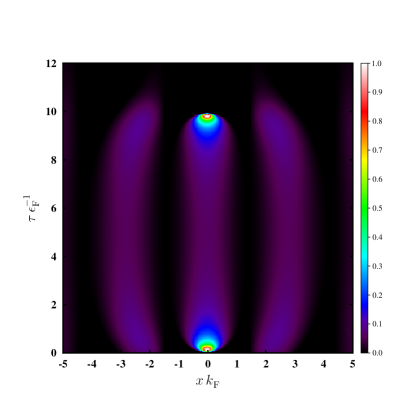
Figure 1: (Color online) Normalized space-time contour plot of the charge density, Eq. (23), for a 1-D electron gas with ${\bf r}_{\rm f}={\bf r}_{\rm i}=0$ and $\tau_{0}\epsilon^{-1}_{\rm F}=10$. Notice, at the points (${\bf r}_{\rm i},0$) and (${\bf r}_{\rm f},\tau_{0}$) it is highly localized, in accordance with the addition and removal of an electron. The stripes or bands are caused by Friedel-like oscillations. See Ref. [Patton and Geller, 2006a] for further details.

Returning to Eq. (II), as has been mentioned and can be seen, finding the exact effective interaction $U_{\rm eff}$ is unobtainable. So one is force to make approximations. The simplest of which is replacing the effective interaction by the bare interaction $U_{\rm eff}\rightarrow U$, this neglects the higher cumulants and other terms of (II) [or (16)]. This actually involves two separate approximations for Eq. (II), one for the saddle-point and the other for $g({\bf r}_{\rm f},{\bf r}_{\rm i},\tau_{0}|\phi_{\rm sp})$. This is because to obtain (II) we assumed knowledge of the exact solution for the saddle-point field. Upon making an approximation for the saddle-point the term $e^{-S_{\rm c}}$ becomes a selective resummation of perturbation theory for $g({\bf r}_{\rm f},{\bf r}_{\rm i},\tau_{0}|\phi_{\rm sp})$. Ultimately, this is what was effectively done in Ref. [Patton and Geller, 2006a] and the failures of the formalism presented there, specifically in the quantum Hall system, can be traced back to these two approximations. Nevertheless, it was also shown that even within these relatively simple approximations the formalism was powerful enough to recover Fermi liquid theory in 2- and 3-D systems, while also obtaining the exact DOS of the 1-D Tomonaga-Luttinger model.

If needed, as in Sec. V, to go beyond this two pronged approximation one should solve for the full $g({\bf r}_{\rm f},{\bf r}_{\rm i},\tau_{0}|\phi_{\rm sp})$, for an approximate $\phi_{\rm sp}$. Doing this and tunneling’s connection to the infrared catastrophe is developed next.

IV Connection to the x-ray edge problem and the x-ray edge limit

Here, it is shown that the saddle-point field is a generalized x-ray edge potential. An x-ray edge potential is a localized time dependent field; generally of the form

$$\phi_{\rm xr}({\bf r},\tau)=U({\bf r})\Theta(\tau_{0}-\tau)\Theta(\tau).$$ (32)

An infrared catastrophe can be caused by the singular screening response of a system to potentials of the form of (32). This behavior is known to be responsible for the singular x-ray optical and photoemission spectra of metals,Mahan (1967); Nozières and De Dominicis (1969); Ohtaka and Tanabe (1990) Anderson’s orthogonality catastrophe,Anderson (1967); Hamann (1971) and even the Kondo effect.Anderson and Yuval (1969); Yuval and Anderson (1970)

The x-ray edge problem, the singular absorption spectra of metals, was predicted by Mahan,Mahan (1967) while studying “excitons” in metals; the hole of the electron-hole pair is created by the absorption of a soft x-ray. It is assumed the hole has a large effective mass and thus the Fermi-sea of the metal responds to a potential of the form of $\phi_{\rm xr}$, where the hole is generated at $\tau=0$ by the absorption of a photon and then later recombines at $\tau=\tau_{0}$.

Note, if $\phi_{\rm sp}=i\phi_{\rm xr}$, apart from phase factors, Eq. (26) is equivalent to the x-ray edge problem,Nozières and De Dominicis (1969) where $G_{\rm sp}$ contains the “exitonic” part and $Z_{\rm xp}$ is the Anderson orthogonality contribution. This connection between tunneling and the x-ray edge field can most easily be seen by starting with the approximate (for transparency only) saddle-point field

$$\phi_{\rm sp}({\bf r},\tau)=i\int d^{D}r^{\prime}\,U({\bf r}-{\bf r}^{\prime})\rho({\bf r}^{\prime},\tau).$$ (33)

As was covered in the previous section, $\rho$ plays the role of an effective charge density of the tunneling electron. Expanding it in multipole moments

$$\rho({\bf r},\tau)=p^{0}(\tau)\delta({\bf r})+p^{1}(\tau)\hat{{\bf r}}{\cdot}\nabla\delta({\bf r})+\cdots,$$ (34)

where $p^{n}(\tau)=\int d^{D}r\,r^{n}\rho({\bf r},\tau)$. It can easily be shownPatton and Geller (2006a) that $p^{0}=\Theta(\tau_{0}-\tau)\Theta(\tau)$. By keeping only the monopole term, the saddle-point field is then

$$\phi_{\rm sp}({\bf r},\tau)\approx iU({\bf r},0)\Theta(\tau_{0}-\tau)\Theta(\tau).$$ (35)

This is the x-ray edge potential, which corresponds to the potential produced if the tunneling particle had an infinite mass. Indeed the saddle-point field is a generalized $\phi_{\rm xr}$, that accounts for both dynamic interactions and recoil of the particle.

We define the so-called x-ray edge limit as the limit where the approximate saddle-point field is taking to be of the form of (35). Thus, the fully interacting Green’s function in this limit is

$$G({\bf r}_{\rm f},{\bf r}_{\rm i},\tau_{0})\sim g({\bf r}_{\rm f},{\bf r}_{\rm i},\tau_{0}|i\phi_{\rm xr}).$$ (36)

or

$$G({\bf r}_{\rm f},{\bf r}_{\rm i},\tau_{0})\sim Z_{\rm sp}(\tau_{0})G_{\rm sp}({\bf r}_{\rm f},{\bf r}_{\rm i},\tau_{0})e^{\int\phi_{\rm xr}n_{0}}.$$ (37)

In this limit, apart from energy shifts, tunneling exactly reduces to the x-ray edge problem. This x-ray edge limit was studied in detail in Refs. [Patton and Geller, 2005, 2006b, 2008] for a 1-D metal and the 2-D quantum Hall system, where qualitative results were found. Of course it is desirable to go beyond this limit and include the full dynamics of the saddle-point (within a given approximation of the integral equation for $\phi_{\rm sp}$). This can be difficult even in the simplest systems; one commonly has to find numerical solutions to the many integral equations, if possible.

V Application to a fractional quantum hall fluid

Because the kinetic energy, and hence the relaxation and recoil of a newly added electron, in the lowest Landau level (LLL) of a quantum Hall system is completely quenched, one would expect this system to be the prototypical example of an infrared catastrophe occurring during tunneling. In the LLL it is known experimentally and theoreticallyEisenstein et al. (1992); Yang and MacDonald (1993); Hatsugai et al. (1993); He et al. (1993); Johansson and Kinaret (1993); Kim and Wen (1994); Aleiner et al. (1995); Haussmann (1996); Wang and Xiong (1999) a pseudogap develops in the DOS near the Fermi energy. In Ref. [Patton and Geller, 2008], it was shown in the x-ray edge limit, $\phi_{\rm sp}\rightarrow\phi_{\rm xr}$, a pseudogap is indeed recovered, but this limit was introduced by hand, based only on plausible physical arguments. It is not obvious using the full formalism presented here that such a result can be obtained.

Here, we apply the method of the previous sections to a two-dimensional electron gas in a quantizing magnetic field. Choosing ${\bf B}=-B{\bf e}_{z}$, and the symmetric gauge ${\bf A}=(By/2){\bf e}_{x}-(Bx/2){\bf e}_{y}$, in the zero-temperature limit the noninteracting Green’s function for the LLL is

$$G_{0}({\bf r},{\bf r}^{\prime},\tau)=\Gamma({\bf r},{\bf r}^{\prime})[\nu-\Theta(\tau)],$$ (38)

where

$$\Gamma({\bf r},{\bf r}^{\prime}) =\sum_{m}\phi_{m}({\bf r})\phi^{*}_{m}({\bf r}^{\prime})$$

$$=\frac{1}{2\pi}\sum_{m=0}^{\infty}\frac{(rr^{\prime})^{m}}{2^{m}m!}e^{im(\theta-\theta^{\prime})}e^{-r^{2}/4}e^{-r^{\prime 2}/4},$$ (39)

and $\phi_{m}({\bf r})$ are the single-particle eigenfunctions (in units where the magnetic length $\ell=\sqrt{\hbar c/eB}=1$), $0<\nu<1$ is the filling factor, and $\Theta(\tau)$ is the Heaviside step function. The charge density, Eq. (23), for this system is therefore

$$\rho({\bf r},\tau)=\frac{e^{-|{\bf r}|^{2}/2}}{2\pi}[\Theta(\tau_{0}-\tau)\Theta(\tau)-\nu].$$ (40)

In systems such as this, with ground-state degeneracy, the leading order approximation for $\phi_{\rm sp}$, $\phi_{\rm sp}({\bf r},\tau)\approx i\int d^{D}r^{\prime}\,U({\bf r}-{\bf r}^{\prime})\rho({\bf r}^{\prime},\tau)$, fails the integrable condition, Eq. (11), for any meaningful interaction in the $\beta\rightarrow\infty$ limit. Therefore, one has to find another approximate solution of (17) by including higher-order terms, in $\phi_{\rm sp}$, to obtain a suitable saddle-point. At a minimum one has to solve the linearized version of (17). This is what we know turn to. Additionally, we will assume a finite inverse-temperature $\beta$, only taking $\beta\rightarrow\infty$ at the end if desired. At finite temperature the LLL Green’s function is

$$G_{0}({\bf r},{\bf r}^{\prime},\tau)=\Gamma({\bf r},{\bf r}^{\prime})[n_{\rm F}(\epsilon_{0}-\mu)-\Theta(\tau)]e^{-(\epsilon_{0}-\mu)\tau},$$ (41)

where $n_{\rm F}(\omega)$ is the Fermi distribution, $\epsilon_{0}$ is the single-particle energy of the lowest Landau level, and the chemical potential $\mu$ is defined such that

$$\nu=\sum_{n=0}^{\infty}\frac{1}{\exp[\beta(\epsilon_{n}-\mu)]+1}.$$ (42)

Note, the Green’s function is aperiodic, $G_{0}(\tau-\beta)=-G_{0}(\tau)$, as it should. The finite-temperature charge density is then

$$\rho({\bf r},\tau)=\frac{e^{-|{\bf r}|^{2}/2}}{2\pi}[\Theta(\tau_{0}-\tau)\Theta(\tau)-n_{\rm F}(\epsilon_{0}-\mu)].$$ (43)

From (17), the linearized integral equation for $\phi_{\rm sp}$, setting ${\bf r}_{\rm f}={\bf r}_{\rm i}=0$, is

$$\phi_{\rm sp}({\bf r},\tau)=i\int d^{2}r^{\prime}\,U({\bf r}-{\bf r}^{\prime})\rho({\bf r^{\prime}},\tau)+\int d^{2}r^{\prime}d^{2}r^{\prime\prime}\int\limits_{0}^{\beta}d\tau^{\prime}\,U({\bf r}-{\bf r}^{\prime})\chi({\bf r}^{\prime},{\bf r}^{\prime\prime},\tau,\tau^{\prime})\phi_{\rm sp}({\bf r}^{\prime\prime},\tau^{\prime})$$

$$+\frac{1}{(2\pi)^{2}}\int d^{2}r^{\prime}d^{2}r^{\prime\prime}\int\limits_{0}^{\beta}d\tau^{\prime}\,U({\bf r}-{\bf r}^{\prime})e^{-|{\bf r}^{\prime}|^{2}/2}e^{-|{\bf r}^{\prime\prime}|^{2}/2}\Big{\{}[\Theta(\tau_{0}-\tau)\Theta(\tau)-n_{\rm F}(\epsilon_{0}-\mu)][\Theta(\tau_{0}-\tau^{\prime})-n_{\rm F}(\epsilon_{0}-\mu)]$$

$$-[n_{\rm F}(\epsilon_{0}-\mu)-\Theta(\tau-\tau^{\prime})][n_{\rm F}(\epsilon_{0}-\mu)-\Theta(\tau_{0}-\tau)]-[n_{\rm F}(\epsilon_{0}-\mu)-\Theta(\tau^{\prime}-\tau)][n_{\rm F}(\epsilon_{0}-\mu)-\Theta(\tau_{0}-\tau^{\prime})]\Big{\}}\phi_{\rm sp}({\bf r}^{\prime\prime},\tau^{\prime}),$$ (44)

where $\chi({\bf r},{\bf r^{\prime}},\tau,\tau^{\prime})=-\frac{n^{\rm F}(1-n^{\rm F})}{(2\pi)^{2}}\,e^{-|{\bf r}-{\bf r}^{\prime}|^{2}/2}.$ In the low-temperature limit, the solution is (see appendix A)

$$\phi_{\rm sp}({\bf r},\tau)\xrightarrow{\beta\rightarrow\infty}\frac{i}{2\pi}\int d^{2}r^{\prime}\,U({\bf r}-{\bf r}^{\prime})e^{-|{\bf r}^{\prime}|^{2}/2}\Theta(\tau_{0}-\tau)\Theta(\tau).$$ (45)

Because this is a valid saddle-point field, we can now determine the interacting Green’s function. Within the cumulant approximation, Sec. III, using (45) gives

$$G(0,0,\tau_{0})\sim\frac{\nu-1}{2\pi}e^{-\lambda(1-\nu)\tau_{0}},$$ (46)

where $\lambda=(4\pi)^{-1}\iint d^{2}rd^{2}r^{\prime}U({\bf r}-{\bf r}^{\prime})e^{-|{\bf r}^{\prime}|^{2}/2}e^{-|{\bf r}|^{2}/2}$. Equation (46) leads to a delta function or “hard-gap” in the DOS

$$N(0,\omega)={\rm const}\times\delta[\omega-\lambda(1-\nu)],$$ (47)

instead of the observed pseudogap. Mathematically a pesudogap can be modeled as a function that decays faster than any power-law at low energy. To obtain this behavior implies that in the time domain the function should exhibit a similar decay rate as $\tau\rightarrow\infty$. Therefore, the fully interacting Green’s function would be expected to be a nonalgebraic and or possibly nonanalytic function of $\tau_{0}$. The cumulant approximation, which is basically a selective resummation of perturbation theory in $\phi_{\rm sp}$ or more explicitly for this case perturbation in $\lambda\tau_{0}$, isn’t powerful enough to capture such behavior; an exact solution of the Dyson equation for the saddle-point Green’s function, Eq. (II), is required for this system.

With (45), the Dyson equation for the saddle-point Green’s function is

$$G_{\rm sp}({\bf r},{\bf r}^{\prime},\tau,\tau^{\prime})=\Gamma({\bf r},{\bf r}^{\prime})\big{[}n_{\rm F}(\epsilon_{0}-\mu)-\Theta(\tau-\tau^{\prime})\big{]}e^{-(\epsilon_{0}-\mu)(\tau-\tau^{\prime})}$$

$$+\frac{1}{2\pi}\int\limits_{0}^{\tau_{0}}d\tau_{1}d^{2}r_{1}d^{2}r_{2}\,\Gamma({\bf r},{\bf r}_{1})\big{[}n_{\rm F}(\epsilon_{0}-\mu)-\Theta(\tau-\tau_{1})\big{]}e^{-(\epsilon_{0}-\mu)(\tau-\tau_{1})}\,U({\bf r}_{1}-{\bf r}_{2})e^{-|{\bf r}_{2}|^{2}/2}G_{\rm sp}({\bf r}_{2},{\bf r}^{\prime},\tau_{1},\tau^{\prime}).$$ (48)

The solution of which isPatton and Geller (2008)

$$G_{\rm sp}({\bf r},{\bf r}^{\prime},\tau,\tau^{\prime})=\sum_{m}\phi_{m}({\bf r})\phi^{*}_{m}({\bf r}^{\prime})a_{m}(\tau,\tau^{\prime}),$$ (49)

where

$$a_{m}(\tau,\tau^{\prime})=\frac{(n_{\rm F}(\epsilon_{0}-\mu)-1)\Theta(\tau-\tau^{\prime})+n_{\rm F}(\epsilon_{0}-\mu)\Theta(\tau^{\prime}-\tau)\exp(-\lambda_{m}\tau_{0})}{1-n_{\rm F}(\epsilon_{0}-\mu)+n_{\rm F}(\epsilon_{0}-\mu)\exp(-\lambda_{m}\tau_{0})}\exp[-\lambda_{m}(\tau-\tau^{\prime})]\exp[-(\epsilon_{0}-\mu)(\tau-\tau^{\prime})]$$ (50)

and

$$\lambda_{m}=\int d^{2}rd^{2}r^{\prime}\,\phi^{*}_{m}({\bf r})U({\bf r}-{\bf r}^{\prime})e^{-|{\bf r}^{\prime}|^{2}/2}\phi_{m}({\bf r}),$$ (51)

are the diagonal matrix elements of the saddle-point interaction in the LLL. For a screened Coulomb potential of the form

$$U({\bf r})=e^{2}\frac{\exp(-\alpha|{\bf r}|)}{|{\bf r}|},$$ (52)

$$\lambda_{m}=e^{2}\int\limits_{0}^{\infty}dk\,\frac{k\exp(-k^{2}/2)}{\sqrt{\alpha^{2}+k^{2}}}_{1}{F}_{1}(1+m,1;-k^{2}/2),$$ (53)

where ${}_{1}F_{1}(a,b;z)$ is the confluent hypergeometric function of the first kind. Experimentally the screening length $\alpha$ would typically be the distance to the nearest gate or to the second 2-D electron gas in bilayer systems.

From appendix B

$$Z_{\rm sp}(\tau_{0})=\prod_{m=0}^{\infty}\big{[}1-n_{\rm F}(\epsilon_{0}-\mu)+n_{\rm F}(\epsilon_{0}-\mu)\exp(-\lambda_{m}\tau_{0})\big{]}.$$ (54)

This finally gives the interacting Green’s function as

$$G(0,0,\tau_{0})\sim Z_{\rm sp}(\tau_{0})G_{\rm sp}(0,0,\tau_{0})\exp\big{(}\nu\alpha^{-1}\tau_{0}\big{)}$$

$$=\frac{1}{2\pi}\prod_{m=1}^{\infty}\big{[}1-n_{\rm F}(\epsilon_{0}-\mu)+n_{\rm F}(\epsilon_{0}-\mu)\exp(-\lambda_{m}\tau_{0})\big{]}$$

$$\times(n_{\rm F}(\epsilon_{0}-\mu)-1)\exp(-\lambda_{0}\tau_{0})\exp\big{(}\nu\alpha^{-1}\tau_{0}\big{)}.$$ (55)

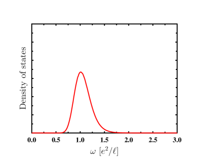
Figure 2: The DOS (up to an overall constant prefactor) of the LLL. Found by analytic continuation of (V), using the experimentally relevent parameters $\beta=10$, $\alpha=.05$, and $\nu=1/3$, in units of $e^{2}/\ell$ and $\ell$.

Figure 2 shows the DOS obtained from (V), by analytically continuation using the maximum entropy method. As can be seen, a pseudogap is present in agreement with experiment. Although, the width of the peak is of the order seen experimentally, the actual location cannot be totally trusted. This is because we have solved for $G_{\rm sp}$ using a long time approximation for $G_{0}$. Then used the solution to find $Z_{\rm sp}$, (see appendix B) but short time information enters into $Z_{\rm sp}$. This is a well-known result from the x-ray edge problem, where unknown energy shifts can occur. The inclusion of higher Landau levels in $G_{0}$ would fix this.

VI Conclusions

By starting with an exact functional integral representation of an interacting Green’s function, followed by a saddle-point approximation, we have shown that the low-energy tunneling behavior of electronic systems is governed by the response of the host system to the time-dependent potential produced by the newly added electron. In the x-ray edge limit the infrared catastrophe occurring during a tunneling event can be exactly mapped to the well-known x-ray edge problem. Within various approximations for the saddle-point we have obtain qualitative as well as quantitative results in a wide spectrum of systems including: Fermi liquids, the Tomonaga-Luttinger liquid, and quantum Hall system.

Future work will involve applying and comparing this method to other exactly solvable models, such as the 1-D Hubbard model and ultimately to the edge of a quantum Hall fluid, where existing theoretical methods fail.

Appendix A Saddle-point field for the Quantum Hall system

Here, we solve for the saddle-point field including the linear term in $\phi_{\rm sp}$ of the integral equation (17). This is needed because the simplest approximation for the saddle-point obtained by keeping only the zeroth order term of Eq. (17) is not in the integration domain of the functional integral. For the quantum Hall system this then reads

$$\phi_{\rm sp}({\bf r},\tau)=i\int d^{2}r^{\prime}\,U({\bf r}-{\bf r}^{\prime})\rho({\bf r^{\prime}},\tau)+\int d^{2}r^{\prime}d^{2}r^{\prime\prime}\int\limits_{0}^{\beta}d\tau^{\prime}\,U({\bf r}-{\bf r}^{\prime})\chi({\bf r}^{\prime},{\bf r}^{\prime\prime},\tau,\tau^{\prime})\phi_{\rm sp}({\bf r}^{\prime\prime},\tau^{\prime})$$

$$+\frac{1}{(2\pi)^{2}}\int d^{2}r^{\prime}d^{2}r^{\prime\prime}\int\limits_{0}^{\beta}d\tau^{\prime}\,U({\bf r}-{\bf r}^{\prime})e^{-|{\bf r}^{\prime}|^{2}/2}e^{-|{\bf r}^{\prime\prime}|^{2}/2}\Big{\{}[\Theta(\tau_{0}-\tau)\Theta(\tau)-n_{\rm F}(\epsilon_{0}-\mu)][\Theta(\tau_{0}-\tau^{\prime})-n_{\rm F}(\epsilon_{0}-\mu)]$$

$$-[n_{\rm F}(\epsilon_{0}-\mu)-\Theta(\tau-\tau^{\prime})][n_{\rm F}(\epsilon_{0}-\mu)-\Theta(\tau_{0}-\tau)]-[n_{\rm F}(\epsilon_{0}-\mu)-\Theta(\tau^{\prime}-\tau)][n_{\rm F}(\epsilon_{0}-\mu)-\Theta(\tau_{0}-\tau^{\prime})]\Big{\}}\phi_{\rm sp}({\bf r}^{\prime\prime},\tau^{\prime}).$$ (56)

Using $\chi({\bf r},{\bf r^{\prime}},\tau,\tau^{\prime})=-\frac{n_{\rm F}(1-n_{\rm F})}{(2\pi)^{2}}\,e^{-|{\bf r}-{\bf r}^{\prime}|^{2}/2}$ and

$$\Theta(\tau_{0}-\tau)\big{[}\Theta(\tau_{0}-\tau^{\prime})-\Theta(\tau-\tau^{\prime})\big{]}-\Theta(\tau^{\prime}-\tau)\Theta(\tau_{0}-\tau^{\prime})=0$$ (57)

gives

$$\phi_{\rm sp}({\bf r},\tau) =i\int d^{2}r^{\prime}\,U({\bf r}-{\bf r}^{\prime})\rho({\bf r^{\prime}},\tau)-\frac{n_{\rm F}(\epsilon_{0}-\mu)[1-n_{\rm F}(\epsilon_{0}-\mu)]}{(2\pi)^{2}}\int d^{2}r^{\prime}d^{2}r^{\prime\prime}\int\limits_{0}^{\beta}d\tau^{\prime}\,U({\bf r}-{\bf r}^{\prime})e^{-|{\bf r}^{\prime}-{\bf r}^{\prime\prime}|^{2}/2}\phi_{\rm sp}({\bf r}^{\prime\prime},\tau^{\prime})$$

$$+\frac{n_{\rm F}(\epsilon_{0}-\mu)\big{[}1-n_{\rm F}(\epsilon_{0}-\mu)\big{]}}{(2\pi)^{2}}\int d^{2}r^{\prime}d^{2}r^{\prime\prime}\int\limits_{0}^{\beta}d\tau^{\prime}\,U({\bf r}-{\bf r}^{\prime})e^{-|{\bf r}^{\prime}|/2}e^{-|{\bf r}^{\prime\prime}|/2}\phi_{\rm sp}({\bf r}^{\prime\prime},\tau^{\prime}).$$ (58)

Introducing the Fourier transforms

$$\phi_{\rm sp}({\bf k},i\Omega_{n})=\int d^{2}r\int\limits_{0}^{\beta}d\tau\,\phi_{\rm sp}({\bf r},\tau)e^{i\Omega_{n}\tau}e^{-i{\bf k}\cdot{\bf r}}\hskip 28.45274pt\text{and}\hskip 28.45274pt\phi_{\rm sp}({\bf r},\tau)=\frac{1}{\beta}\sum_{n}\int\frac{d^{2}k}{(2\pi)^{2}}\phi_{\rm sp}({\bf k},i\Omega_{n})e^{-i\Omega_{n}\tau}e^{i{\bf k}\cdot{\bf r}},$$ (59)

where $i\Omega_{n}$ is a bonsonic frequency, the integral equation in Fourier space is

$$\phi_{\rm sp}({\bf k},i\Omega_{n}) =iU({\bf k})\rho({\bf k},i\Omega_{n})-\frac{n_{\rm F}(\epsilon_{0}-\mu)[1-n_{\rm F}(\epsilon_{0}-\mu)]}{(2\pi)^{2}}U({\bf k})e^{-|{\bf k}|^{2}/2}\phi_{\rm sp}({\bf k},i\Omega_{n^{\prime}})\beta\delta_{i\Omega_{n^{\prime}},0}\delta_{i\Omega_{n},0}$$

$$+\frac{n_{\rm F}(\epsilon_{0}-\mu)[1-n_{\rm F}(\epsilon_{0}-\mu)]}{(2\pi)^{2}}U({\bf k})e^{-|{\bf k}|^{2}/2}\int d^{2}k\,^{\prime}e^{-|{\bf k}^{\prime}|^{2}/2}\phi_{\rm sp}({\bf k}^{\prime},i\Omega_{n^{\prime}})\beta\delta_{i\Omega_{n^{\prime}},0}\delta_{i\Omega_{n},0}.$$ (60)

Thus for $i\Omega_{n}\neq 0$

$$\phi_{\rm sp}({\bf k},i\Omega_{n}\neq 0)=iU({\bf k})\rho({\bf k},i\Omega_{n}\neq 0)$$ (61)

and for $i\Omega_{n}=0$

$$\phi_{\rm sp}({\bf k},i\Omega_{n}=0) =iU({\bf k})\rho({\bf k},i\Omega_{n}=0)-\frac{\beta}{(2\pi)^{2}}n_{\rm F}(\epsilon_{0}-\mu)[1-n_{\rm F}(\epsilon_{0}-\mu)]U({\bf k})e^{-|{\bf k}|^{2}/2}\phi_{\rm sp}({\bf k},i\Omega_{n}=0)$$

$$+\frac{\beta}{(2\pi)^{2}}n_{\rm F}(\epsilon_{0}-\mu)[1-n_{\rm F}(\epsilon_{0}-\mu)]U({\bf k})e^{-|{\bf k}|^{2}/2}\int d^{2}k^{\prime}e^{-|{\bf k}^{\prime}|^{2}/2}\phi_{\rm sp}({\bf k}^{\prime},i\Omega_{n}=0).$$ (62)

or

$$\phi_{\rm sp}({\bf k},i\Omega_{n}=0) =\frac{iU({\bf k})\rho({\bf k},i\Omega_{n}=0)}{1+\frac{\beta}{(2\pi)^{2}}n_{\rm F}(\epsilon_{0}-\mu)[1-n_{\rm F}(\epsilon_{0}-\mu)]U({\bf k})e^{-|{\bf k}|^{2}/2}}$$

$$+\frac{\beta}{(2\pi)^{2}}\frac{n_{\rm F}(\epsilon_{0}-\mu)[1-n_{\rm F}(\epsilon_{0}-\mu)]U({\bf k})e^{-|{\bf k}|^{2}/2}}{1+\frac{\beta}{(2\pi)^{2}}n_{\rm F}(\epsilon_{0}-\mu)[1-n_{\rm F}(\epsilon_{0}-\mu)]U({\bf k})e^{-|{\bf k}|^{2}/2}}\int d^{2}k^{\prime}e^{-|{\bf k}^{\prime}|^{2}/2}\phi_{\rm sp}({\bf k}^{\prime},i\Omega_{n}=0)$$ (63)

This is a Fredholm integral equation with a degenerate kernel whose solution is simply given byPolyamin and Manzhirov (1998)

$$\phi_{\rm sp}({\bf k},i\Omega_{n}=0) =\frac{iU({\bf k})\rho({\bf k},i\Omega_{n}=0)}{1+\frac{\beta}{(2\pi)^{2}}n_{\rm F}(\epsilon_{0}-\mu)[1-n_{\rm F}(\epsilon_{0}-\mu)]U({\bf k})e^{-|{\bf k}|^{2}/2}}$$

$$+A(i\Omega_{n}=0)\frac{\beta}{(2\pi)^{2}}\frac{n_{\rm F}(\epsilon_{0}-\mu)[1-n_{\rm F}(\epsilon_{0}-\mu)]U({\bf k})e^{-|{\bf k}|^{2}/2}}{1+\frac{\beta}{(2\pi)^{2}}n_{\rm F}(\epsilon_{0}-\mu)[1-n_{\rm F}(\epsilon_{0}-\mu)]U({\bf k})e^{-|{\bf k}|^{2}/2}}$$ (64)

where

$$A(i\Omega_{n}=0)=\frac{\displaystyle{\int}d^{2}k\,\frac{iU({\bf k})\rho({\bf k},i\Omega_{n}=0)e^{-|{\bf k}|^{2}/2}}{1+\frac{\beta}{(2\pi)^{2}}n_{\rm F}(\epsilon_{0}-\mu)[1-n_{\rm F}(\epsilon_{0}-\mu)]U({\bf k})e^{-|{\bf k}|^{2}/2}}}{\displaystyle{1-\frac{\beta}{(2\pi)^{2}}\int d^{2}k\frac{n_{\rm F}(\epsilon_{0}-\mu)[1-n_{\rm F}(\epsilon_{0}-\mu)]U({\bf k})e^{-|{\bf k}|^{2}/2}e^{-|{\bf k}|^{2}/2}}{1+\frac{\beta}{(2\pi)^{2}}n_{\rm F}(\epsilon_{0}-\mu)[1-n_{\rm F}(\epsilon_{0}-\mu)]U({\bf k})e^{-|{\bf k}|^{2}/2}}}}.$$ (65)

Converting back to $\tau$ space

$$\phi_{\rm sp}({\bf k},\tau)=\frac{1}{\beta}\sum_{n\in\mathbb{Z}}iU({\bf k})\rho({\bf k},i\Omega_{n})e^{-i\Omega_{n}\tau}-\beta^{-1}iU({\bf k})\rho({\bf k},i\Omega_{n}=0)+\beta^{-1}\phi_{\rm sp}({\bf k},i\Omega_{n}=0),$$ (66)

where the $i\Omega=0$ term has been subtracted from the sum over frequencies. In the $\beta\rightarrow\infty$ limit

$$\phi_{\rm sp}({\bf k},\tau)\rightarrow\frac{i}{2\pi}U({\bf k})e^{-|{\bf k}|^{2}/2}\Theta(\tau_{0}-\tau)\Theta(\tau),$$ (67)

or in real space

$$\phi_{\rm sp}({\bf r},\tau)=\frac{i}{2\pi}\int d^{2}r^{\prime}\,U({\bf r}-{\bf r}^{\prime})e^{-|{\bf r}^{\prime}|^{2}/2}\Theta(\tau_{0}-\tau)\Theta(\tau).$$ (68)

This is the form of the saddle-point field that is used in Sec. V.

Appendix B Saddle-Point S-matrix

Here, the saddle-point scattering matrix $Z_{\rm sp}$ is found from $G_{\rm sp}$. This is a straightforward generalization of the coupling constant integration trick found in Ref. [Nozières and De Dominicis, 1969].

From the linked cluster theorem,

$$Z_{\rm sp}=\big{\langle}Te^{i\int d\tau d^{D}r\ \phi_{\rm sp}({\bf r},t)\hat{n}({\bf r},\tau)}\big{\rangle}_{0}=e^{M},$$ (69)

where

$$M=\sum_{l=1}^{\infty}\frac{i^{l}}{l}\int d\tau_{1}d^{D}r_{1}\cdots d\tau_{l}d^{D}r_{l}\,\phi_{\rm sp}({\bf r}_{1},\tau_{1})\cdots\phi_{\rm sp}({\bf r}_{l},\tau_{l})\left<T\hat{n}({\bf r}_{1},\tau_{1})\cdots\hat{n}({\bf r}_{l},\tau_{l})\right>_{{\rm different\,connected}}$$ (70)

or

$$M=i\sum_{l=1}^{\infty}\frac{1}{l}\int d\tau_{1}d^{D}r_{1}\cdots d\tau_{l}d^{D}r_{l}\,\phi_{\rm sp}({\bf r}_{1},\tau_{1})\cdots\phi_{\rm sp}({\bf r}_{l},\tau_{1})G_{0}({\bf r}_{1},{\bf r}_{l},\tau_{1},\tau_{l})\cdots G_{0}({\bf r}_{l},{\bf r}_{1},\tau_{l},\tau_{1}^{+}).$$ (71)

Changing the summation limit leads to

$$M=i\sum_{l=0}^{\infty}\frac{1}{l+1}\int d\tau_{1}d^{D}r_{1}\cdots d\tau_{l+1}d^{D}r_{l+1}\phi_{\rm sp}({\bf r}_{1},\tau_{1})\cdots\phi_{\rm sp}({\bf r}_{l+1},\tau_{l+1})G_{0}({\bf r}_{1},{\bf r}_{l+1},\tau_{1},\tau_{l+1})\cdots G_{0}({\bf r}_{l+1},{\bf r}_{1},\tau_{l+1},\tau_{1}^{+}).$$ (72)

Introducing

$${G}^{\xi}_{\rm sp}({\bf r},{\bf r}^{\prime},\tau,\tau^{+})=G_{0}({\bf r},{\bf r}^{\prime},\tau,\tau^{+})-i\,\xi\int d\tau^{\prime\prime}d^{D}r^{\prime\prime}\,G_{0}({\bf r},{\bf r}^{\prime\prime},\tau,\tau^{\prime\prime})\phi_{\rm sp}({\bf r}^{\prime\prime},\tau^{\prime\prime})G^{\xi}_{\rm sp}({\bf r}^{\prime\prime},{\bf r}^{\prime},\tau^{\prime\prime},\tau^{+})$$ (73)

and using

$$\frac{1}{l+1}=\int_{0}^{1}d\xi\ \xi^{l}$$ (74)

Eq. (72) can be written simply as

$$M=i\int d\tau\int d^{D}r\int_{0}^{1}d\xi\,\phi_{\rm sp}({\bf r},\tau)G^{\xi}_{\rm sp}({\bf r},{\bf r},\tau,\tau^{+}).$$ (75)

Reinstating spin for completeness gives

$$M=i\sum_{\sigma}\int d\tau\int d^{D}r\int_{0}^{1}d\xi\,\phi_{\rm sp}({\bf r},\tau)G^{\xi}_{\rm sp}({\bf r},{\bf r},\tau,\tau^{+},\sigma).$$ (76)

References

• Gross and Dreizler (1995) E. Gross and R. Dreizler, Density Functional Theory (Plenum Press, New York, 1995).
• Haldane (1981) F. D. M. Haldane, J. Phys. C 14, 2585 (1981).
• White (1992) S. R. White, Phys. Rev. Lett. 69, 2863 (1992).
• Georges et al. (1996) A. Georges, G. Kotliar, W. Krauth, and M. J. Rozenberg, Rev. Mod. Phys. 68, 13 (1996).
• Rubtsov et al. (2008) A. N. Rubtsov, M. I. Katsnelson, and A. I. Lichtenstein, Phys. Rev. B 77, 033101 (2008).
• Goldman (2001) V. J. Goldman, Phys. Rev. Lett. 86, 5841 (2001).
• Wian et al. (2002) X. Wian, K. Yang, and E. H. Rezayi, Phys. Rev. Lett. 88, 056802 (2002).
• Wan et al. (2005) X. Wan, F. Evers, and E. H. Rezayi, Phys. Rev. Lett. 94, 166804 (2005).
• Grayson et al. (1998) M. Grayson, D. C. Tsui, L. N. Pfeiffer, K. W. West, and A. M. Chang, Phys. Rev. Lett. 80, 1062 (1998).
• Levitov and Shytov (1997) L. S. Levitov and A. V. Shytov, JETP Lett. 66, 216 (1997).
• Mahan (1967) G. D. Mahan, Phys. Rev. 163, 612 (1967).
• Nozières and De Dominicis (1969) P. Nozières and C. T. De Dominicis, Phys. Rev. 178, 1097 (1969).
• Anderson (1967) P. W. Anderson, Phys. Rev. Lett. 18, 1049 (1967).
• Hamann (1971) D. R. Hamann, Phys. Rev. Lett. 26, 1030 (1971).
• Yuval and Anderson (1970) G. Yuval and P. W. Anderson, Phys. Rev. B 1, 1522 (1970).
• Patton and Geller (2008) K. R. Patton and M. R. Geller, J. Phys.: Condens. Matter 20, 295210 (2008).
• Patton and Geller (2006a) K. R. Patton and M. R. Geller, Phys. Rev. B 73, 125416 (2006a).
• Patton and Geller (2006b) K. R. Patton and M. R. Geller, Phys. Rev. B 73, 245306 (2006b).
• Patton and Geller (2005) K. R. Patton and M. R. Geller, Phys. Rev. B 72, 125108 (2005).
• Nozières and De Dominicis (1969) P. Nozières and C. T. De Dominicis, Phys. Rev. 178, 1097 (1969).
• Ohtaka and Tanabe (1990) K. Ohtaka and Y. Tanabe, Rev. Mod. Phys. 62, 929 (1990).
• Anderson and Yuval (1969) P. W. Anderson and G. Yuval, Phys. Rev. Lett. 23, 89 (1969).
• Eisenstein et al. (1992) J. P. Eisenstein, L. N. Pfeiffer, and K. W. West, Phys. Rev. Lett. 69, 3804 (1992).
• Yang and MacDonald (1993) S.-R. E. Yang and A. H. MacDonald, Phys. Rev. Lett. 70, 4110 (1993).
• Hatsugai et al. (1993) Y. Hatsugai, P.-A. Bares, and X.-G. Wen, Phys. Rev. Lett. 71, 424 (1993).
• He et al. (1993) S. He, P. M. Platzman, and B. I. Halperin, Phys. Rev. Lett. 71, 777 (1993).
• Johansson and Kinaret (1993) P. Johansson and J. M. Kinaret, Phys. Rev. Lett. 71, 1435 (1993).
• Kim and Wen (1994) Y. B. Kim and X. G. Wen, Phys. Rev. B 50, 8078 (1994).
• Aleiner et al. (1995) I. L. Aleiner, H. U. Baranger, and L. I. Glazman, Phys. Rev. Lett. 74, 3435 (1995).
• Haussmann (1996) R. Haussmann, Phys. Rev. B 53, 7357 (1996).
• Wang and Xiong (1999) Z. Wang and S. Xiong, Phys. Rev. Lett. 83, 828 (1999).
• Polyamin and Manzhirov (1998) A. D. Polyamin and A. V. Manzhirov, Handbook of Integral Equations (CRC Press, Boca Raton, 1998).