Three-dimensional simulations of molecular cloud fragmentation regulated by magnetic fields and ambipolar diffusion

Abstract

We employ the first fully three-dimensional simulation to study the role of magnetic fields and ion-neutral friction in regulating gravitationally-driven fragmentation of molecular clouds. The cores in an initially subcritical cloud develop gradually over an ambipolar diffusion time while the cores in an initially supercritical cloud develop in a dynamical time. The infall speeds on to cores are subsonic in the case of an initially subcritical cloud, while an extended ($\ga 0.1$ pc) region of supersonic infall exists in the case of an initially supercritical cloud. These results are consistent with previous two-dimensional simulations. We also found that a snapshot of the relation between density ($\rho$) and the strength of the magnetic field ($B$) at different spatial points of the cloud coincides with the evolutionary track of an individual core. When the density becomes large, both relations tend to $B\propto\rho^{0.5}$.

1 Introduction

Magnetic fields in molecular clouds play an important role in the early stages of star formation. They may regulate the cloud fragmentation process, moderate the infall motions on to density peaks, control angular momentum evolution through magnetic braking, launch jets from the near-protostellar environment, and possibly determine a finite mass reservoir for star formation by limiting accretion from a magnetically-dominated envelope. The prevailing macroturbulence in molecular cloud envelopes also likely represents magnetohydrodynamic motions. This paper concerns itself with the first two issues above: we employ the first fully three-dimensional simulation to study the role of magnetic fields and ion-neutral friction in regulating gravitationally-driven fragmentation and infall.

The relative strengths of gravity and the magnetic field can be quantified through the mass-to-flux ratio $M/\Phi$. There exists a critical mass-to-flux ratio $(M/\Phi)_{\rm crit}$ (Mestel & Spitzer, 1956; Strittmatter, 1966; Mouschovias & Spitzer, 1976; Tomisaka, Ikeuchi, & Nakamura, 1988) such that if $M/\Phi>(M/\Phi)_{\rm crit}$, a pressure-bounded cloud is supercritical and is prone to indefinite collapse if the external pressure exceeds some value. This behaviour is analogous to that of the nonmagnetic Bonnor-Ebert sphere. Conversely, if $M/\Phi<(M/\Phi)_{\rm crit}$, a cloud is subcritical and cannot collapse even in the limit of infinite external pressure, as long as magnetic flux-freezing applies. A similar condition $M/\Phi<(M/\Phi)_{\rm crit}=(2\pi G^{1/2})^{-1}$ is required for unconditional stability of an infinite uniform (in $x,y$) layer that is flattened along the $z$-direction of a background magnetic field (Nakano & Nakamura, 1978). The various numerical values of $(M/\Phi)_{\rm crit}$ differ by small factors of order unity, and we adopt the result of Nakano & Nakamura (1978) since their model closely resembles the initial state in our calculation.

Magnetic field strength measurements through the Zeeman effect reveal that the mass-to-flux ratios are clustered about the critical value for collapse (Crutcher, 1999, 2004; Shu et al., 1999) and that there is also an approximate equipartition between the absolute values of gravitational energy and nonthermal (hereafter, “turbulent”) energy (Myers & Goodman, 1988; Basu, 2000). Measurements of polarized emission from dust grains, which reveal the field morphology, generally indicate that the field in cloud cores is well ordered and not dominated by turbulent motions, with application of the Chandrasekhar-Fermi method yielding mass-to-flux ratios near the critical value (Lai et al., 2001, 2002; Crutcher, Nutter, & Ward-Thompson, 2004; Curran et al., 2004; Kirk, Ward-Thompson, & Crutcher, 2006).

Mestel & Spitzer (1956) pointed out that even if clouds are magnetically supported, ambipolar diffusion (resulting from ion-neutral slip) will cause the support to be lost and stars to form. More specifically, a medium with a subcritical mass-to-flux ratio will still undergo a gravitationally-driven instability, occurring on the ambipolar diffusion time scale rather than the dynamical time scale (Langer, 1978; Zweibel, 1998; Ciolek & Basu, 2006). The length scale of the instability is essentially the Jeans scale in the limit of highly subcritical clouds (the same length scale as for highly supercritical fragmentation) but can be much larger when the mass-to-flux ratio is close to the critical value (Ciolek & Basu, 2006). Most nonlinear calculations of ambipolar diffusion driven evolution have focused on a single axisymmetric core, but newer models focus on a fragmentation process that results in the formation of multiple cores and somewhat irregular density and velocity structure. Indebetouw & Zweibel (2000) carried out a two-dimensional simulation of an infinitesimally-thin sheet threaded by an initially perpendicular magnetic field. Starting with slightly subcritical initial conditions, they followed the initial growth of mildly elongated fragments which occurred on a time scale intermediate between the dynamical time associated with supercritical collapse and the ambipolar diffusion time-scale associated with highly subcritical clouds. Basu & Ciolek (2004) carried out two-dimensional simulations of a magnetized sheet in the thin-disc approximation, which incorporates a finite disc half-thickness $Z$ consistent with hydrostatic equilibrium and thereby includes the effect of magnetic pressure. They studied a model which had an initially critical mass-to-flux ratio and another which was supercritical by a factor of two. One of their main results was that the critical model had subsonic (maximum speed $\approx 0.5c_{\rm s}$, where $c_{\rm s}$ is the isothermal sound speed) infall, while the decidedly supercritical cloud had infall speeds $\ga 1c_{\rm s}$ on scales $\sim 0.1$ pc from the core centres. This is a significant observationally-testable difference between dynamical (supercritical) fragmentation and ambipolar-diffusion regulated (critical or subcritical) fragmentation. Yet another mode of fragmentation is the so-called turbulent fragmentation, which in fact corresponds to collapse driven by a strong external compression. Li & Nakamura (2004) and Nakamura & Li (2005) have studied this process for a magnetized sheet using the thin-disc approximation, and including the effect of ion-neutral friction. They find that a mildly subcritical cloud can undergo locally rapid ambipolar diffusion and form multiple fragments because of an initial large-scale highly supersonic compression wave. The core formation occurs on a crossing time of the simulation box, which is related to the dynamical time. Li & Nakamura (2004) estimate that such a process can simultaneously maintain a relatively low efficiency of star formation, as is required by observations (Lada & Lada, 2003).

In this paper, we study the three-dimensional extension of models such as those of Indebetouw & Zweibel (2000) and Basu & Ciolek (2004). The self-consistent calculation of the vertical structure of the cloud allows us to test the predictions of two-dimensional models as well as to make some new predictions. We model clouds that are either decidedly supercritical or subcritical and study the evolution after the introduction of small-amplitude perturbations. The case of compression-induced collapse will be studied in a separate paper. We note that our three-dimensional model is not a cubic region but rather a flattened three-dimensional layer that is consistent with the expected settling of gas along the direction of the magnetic field. In reality, we believe that our modeled region would represent the dense midplane of a larger more turbulent cloud. As demonstrated by the one-dimensional models of Kudoh & Basu (2003, 2006), the turbulent motions in a stratified magnetized cloud develop the largest amplitude motions in the outer low-density envelope, while maintaining transonic or subsonic motions near the midplane. We believe that the fragmentation process as modeled in this paper may proceed while long-lived turbulent motions continue on larger scales.

2 Numerical Model

2.1 Basic Equations

We solve the three-dimensional magnetohydrodynamic (MHD) equations including self-gravity and ambipolar diffusion, assuming that neutrals are much more numerous than ions:

$$\frac{\partial\rho}{\partial t}+\mbox{\boldmath$v$}\cdot\nabla\rho=-\rho\nabla\cdot\mbox{\boldmath$v$},$$ (1)

$$\frac{\partial\mbox{\boldmath$v$}}{\partial t}+(\mbox{\boldmath$v$}\cdot\nabla)\mbox{\boldmath$v$}=-\frac{1}{\rho}\nabla p+\frac{1}{c\rho}\mbox{\boldmath$j$}\times\mbox{\boldmath$B$}-\nabla\psi,$$ (2)

$$\frac{\partial\mbox{\boldmath$B$}}{\partial t}=\nabla\times(\mbox{\boldmath$v$}\times\mbox{\boldmath$B$})+\nabla\times\left[\frac{\tau_{ni}}{c\rho}(\mbox{\boldmath$j$}\times\mbox{\boldmath$B$})\times\mbox{\boldmath$B$}\right],$$ (3)

$$\mbox{\boldmath$j$}=\frac{c}{4\pi}\nabla\times\mbox{\boldmath$B$},$$ (4)

$$\nabla^{2}\psi=4\pi G\rho,$$ (5)

$$p=c_{s}^{2}\rho,$$ (6)

where $\rho$ is the density of neutral gas, $p$ is the pressure, $v$ is the velocity, $B$ is the magnetic field, $j$ is the electric current density, $\psi$ is the self-gravitating potential, and $c_{s}$ is the sound speed. Instead of solving a detailed energy equation, we assume isothermality for each Lagrangian fluid particle (Kudoh & Basu, 2003, 2006):

$$\frac{dc_{s}}{dt}=\frac{\partial c_{s}}{\partial t}+\mbox{\boldmath$v$}\cdot\nabla c_{s}=0.$$ (7)

For the neutral-ion collision time in equation (3) and associated quantities, we follow Basu & Mouschovias (1994), so that

$$\tau_{ni}=1.4\,\frac{m_{i}+m_{n}}{\rho_{i}\langle\sigma w\rangle_{in}},$$ (8)

where $\rho_{i}$ is the density of ions and $\langle\sigma w\rangle_{in}$ is the average collisional rate between ions of mass $m_{i}$ and neutrals of mass $m_{n}$. Here, we use typical values of HCO⁺-H₂ collisions, for which $\langle\sigma w\rangle_{in}=1.69\times 10^{-9}$ cm^-3s^-1 and $m_{i}/m_{n}=14.4$. We also assume that the ion density $\rho_{i}$ is determined by the approximate relation (Elmegreen, 1979; Nakano, 1979)

$$\rho_{i}=m_{i}K\left(\frac{\rho/m_{n}}{10^{5}\mbox{cm${}^{-3}$}}\right)^{k},$$ (9)

where we assume $K=3\times 10^{-3}$cm^-3 and $k=0.5$ throughout this paper.

2.2 Initial Conditions

As an initial condition, we assume hydrostatic equilibrium of a self-gravitating one-dimensional cloud along $z$-direction (Kudoh & Basu, 2003, 2006). The hydrostatic equilibrium is calculated from equations

$$\frac{dp}{dz}=\rho g_{z},$$ (10)

$$\frac{dg_{z}}{dz}=-4\pi G\rho,$$ (11)

$$p=c_{s}^{2}\rho,$$ (12)

subject to the boundary conditions

$$g_{z}(z=0)=0,\ \ \rho(z=0)=\rho_{0},\ \ p(z=0)=\rho_{0}c_{s0}^{2}$$ (13)

where $\rho_{0}$ and $c_{s0}$ are the initial density and sound speed at $z=0$. If the initial sound speed (temperature) is uniform throughout the region, we have the following analytic solution $\rho_{S}$ found by Spitzer (1942):

$$\rho_{S}(z)=\rho_{0}\,\mbox{sech}^{2}(z/H_{0}),$$ (14)

where

$$H_{0}=\frac{c_{s0}}{\sqrt{2\pi G\rho_{0}}}$$ (15)

is the scale height. However, an isothermal molecular cloud is usually surrounded by warm material, such as neutral hydrogen gas. Hence, we assume the initial sound speed distribution to be

$$c_{s}^{2}(z)=c_{s0}^{2}+\frac{1}{2}(c_{sc}^{2}-c_{s0}^{2})\left[1+\tanh\left(\frac{|z|-z_{c}}{z_{d}}\right)\right]$$ (16)

where we take $c_{sc}^{2}=10\,c_{s0}^{2}$, $z_{c}=2H_{0}$, and $z_{d}=0.1H_{0}$ throughout the paper. By using this sound speed distribution, we can solve equations (10)-(12) numerically. The initial density distribution of the numerical solution shows that it is almost the same as Spitzer’s solution for $0\leq z\leq z_{c}$.

We also assume that the initial magnetic field is uniform along the $z$-direction:

$$B_{z}=B_{0},\ \ B_{x}=B_{y}=0,$$ (17)

where $B_{0}$ is constant.

In this equilibrium sheet-like gas, we input a random velocity perturbation (Miyama, Narita, & Hayashi, 1987b) at each grid point:

$$v_{x}=0.1c_{s0}R_{m},\ \ v_{y}=0.1c_{s0}R_{m},\ \ v_{z}=0.0$$ (18)

where $R_{m}$ is a random number chosen uniformly from the range [-1,1]. The $R_{m}$’s for each of $v_{x}$ and $v_{y}$ are independent realizations. However, each model presented in this paper uses the same pair of realizations of $R_{m}$ for generating the initial perturbations.

2.3 Numerical Parameters

A set of fundamental units for this problem are $c_{s0}$, $H_{0}$, and $\rho_{0}$. These yield a time unit $t_{0}=H_{0}/c_{s0}$. The initial magnetic field strength introduces one dimensionless free parameter,

$$\beta_{0}\equiv\frac{8\pi p_{0}}{B_{0}^{2}}=\frac{8\pi\rho_{0}c_{s0}^{2}}{B_{0}^{2}},$$ (19)

the ratio of gas to magnetic pressure at $z=0$.

In the sheet-like equilibrium cloud with a vertical magnetic field, $\beta_{0}$ is related to the mass-to-flux ratio for Spitzer’s self-gravitating cloud. The mass-to-flux ratio normalized to the critical value is

$$\mu_{S}\equiv 2\pi G^{1/2}\frac{\Sigma_{S}}{B_{0}}$$ (20)

where

$$\Sigma_{S}=\int_{-\infty}^{\infty}\rho_{S}dz=2\rho_{0}H_{0}$$ (21)

is the column density of Spitzer’s self-gravitating cloud. Therefore,

$$\beta_{0}=\mu_{S}^{2}.$$ (22)

Although the initial cloud we used is not exactly the same as the Spitzer cloud, $\beta_{0}$ is a good indicator to whether or not the magnetic field can prevent gravitational instability (Nakano & Nakamura, 1978).

Dimensional values of all quantities can be found through a choice of $\rho_{0}$ and $c_{s0}$. For example, for $c_{s0}=0.2$ km s^-1 and $n_{0}=\rho_{0}/m_{n}=10^{4}$ cm^-3, we get $H_{0}=0.05$ pc, $t_{0}=2.5\times 10^{5}$ yr, and $B_{0}=20\,\mu$G if $\beta_{0}=1$.

2.4 Numerical Technique

In order to solve the equations numerically, we use the CIP method (Yabe & Aoki, 1991; Yabe, Xiao, & Utsumi, 2001) for equations (1), (2) and (7), and the method of characteristics-constrained transport (MOCCT; Stone & Norman (1992)) for equation (3), including an explicit integration of the ambipolar diffusion term. The combination of the CIP and MOCCT methods is summarized in Kudoh, Matsumoto, & Shibata (1999) and Ogata et al. (2004). It includes the CCUP method (Yabe & Wang, 1991) for the calculation of gas pressure, in order to get more numerically stable results. The numerical code in this paper is based on that of Ogata et al. (2004).

In this paper, the ambipolar diffusion term is only included when the density is greater than a certain value, $\rho_{cr}$. We let $\rho_{cr}=0.3\rho_{0}$ both for numerical convenience and due to the physical idea that the low density region is affected by external ultraviolet radiation so that the ionization fraction becomes large, i.e. $\tau_{ni}$ becomes small (Ciolek & Mouschovias, 1995). Under this assumption, the upper atmosphere of the sheet-like cloud is not affected by ambipolar diffusion. This simple assumption helps to avoid very small time-steps due to the low density region in order to maintain stability of the explicit numerical scheme.

We used a mirror-symmetric boundary condition at $z=0$ and periodic boundaries in the $x$ and $y$-directions. At the upper boundary at $z=z_{\rm out}=4H_{0}$, we also used a mirror-symmetric boundary except when we solve the gravitational potential. This symmetric condition is just for numerical convenience. However, because the results we show later in this paper are consistent with previous two-dimensional simulations, we believe that the boundary conditions do not affect the result significantly. The Poisson equation (5) is solved by the Greens function method to compute the gravitational kernels in $z$-direction, along with a Fourier transform method in the $x$ and $y$-directions (Miyama, Narita, & Hayashi, 1987b). This method of solving the Poisson equation allows us to find the gravitational potential of a vertically isolated cloud within $|z|<z_{\rm out}$.

The computational region is $|x|,|y|\leq 8\pi H_{0}$ and $0\leq z\leq 4H_{0}$. The number of grid points for each direction is $(N_{x},N_{y},N_{z})=(64,64,40)$. Since the most unstable wavelength for no magnetic field is about $4\pi H_{0}$ (Miyama, Narita, & Hayashi, 1987a), we have 16 grid points within this wavelength. We have also 10 grid points within the scale height of the initial cloud in the $z$-direction. While this is not a high-resolution simulation, we believe that we have the minimum number of grid points to study the gravitational instability, especially by using the code based on CIP (Ogata et al., 2004). The maximum computational time, which occurs for the case of the subcritical cloud, is about 85 hours of CPU time using a single processor of the VPP5000 in the National Astronomical Observatory of Japan.

3 Results

Figure 1: The time evolution of the density at the location where the density reaches its maximum value in each simulation. Each line shows a case of different $\beta_{0}$.

Figure 1 shows the time evolution of the density at the location where the density reaches its maximum value in each simulation. The simulations are stopped when the maximum density is about $30\rho_{0}$. Each line shows a case of different $\beta_{0}$. When $\beta_{0}$ is 100 or 4, the magnetic field is not strong enough to suppress the self-gravitational instability of the cloud. In these cases, the density evolves rapidly, over the sound-crossing time of the most unstable wavelength ($\sim 4\pi H_{0}$). However, when $\beta_{0}=0.25$, the cloud is self-gravitationally stable unless ion-neutral slip is present. Therefore, the density evolves gradually over the diffusion time of the magnetic field. According to the two-dimensional linear analysis by Ciolek & Basu (2006), the evolutionary time scale of a significantly subcritical cloud is about ten times longer than the dynamical time, for a standard ionization fraction, as used here. Our numerical result is consistent with their analysis.

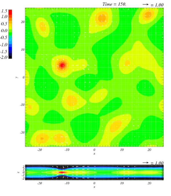
Figure 2: The logarithmic density contours for $\beta_{0}=0.25$ at $t=150$. Arrows show velocity vectors on each cross section. Upper panel shows the cross section at $z=0$, and the lower panel shows the cross section at $y=4.3$.

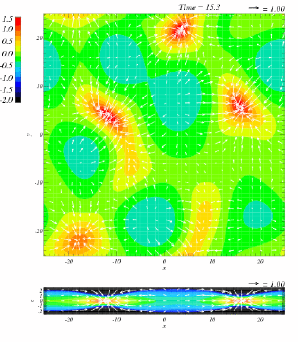
Figure 3: The logarithmic density contours for $\beta_{0}=4$ at $t=15.3$. Arrows show velocity vectors on each cross section. Upper panel shows the cross section at $z=0$, and the lower panel shows the cross section at $y=5.1$.

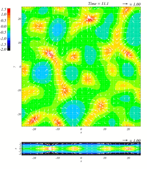
Figure 4: The logarithmic density contours for $\beta_{0}=100$ at $t=11.1$. Arrows show velocity vectors on each cross section. Upper panel shows the cross section at $z=0$, and the lower panel shows the cross section at $y=5.1$.

Figure 2, Figure 3, and Figure 4 show the logarithmic density contours for $\beta_{0}=0.25$ at $t=150$, $\beta_{0}=4$ at $t=15.3$, and $\beta_{0}=100$ at $t=11.1$ respectively. Each upper panel shows the cross section at $z=0$, and the lower panel shows the cross section at $y=4.3$ for $\beta_{0}=0.25$, $y=5.1$ for $\beta_{0}=4$, and $y=5.1$ for $\beta_{0}=100$ respectively. The values of $y$ for the lower panels are chosen so that the vertical cut passes through at least one dense core. (In these numerical simulations, we use the term ”core” to refer to the region where the density is greater than the mean background density by about a factor of 3.) The size of cores for $\beta_{0}=4$ is bigger than that of $\beta_{0}=100$. The size becomes smaller again when the magnetic field is stronger than critical ($\beta_{0}=0.25$). This result is consistent with the two-dimensional linear analysis of Ciolek & Basu (2006), who found a hybrid mode for critical or mildly supercritical clouds in which the combined effect of field-line dragging and magnetic restoring forces enforce a larger than usual fragmentation scale. Arrows show velocity vectors on each cross section. Maximum velocities become supersonic for $\beta_{0}=4$ and $\beta_{0}=100$, but remain subsonic for $\beta_{0}=0.25$. This is also consistent with the two-dimensional numerical simulations of Basu & Ciolek (2004).

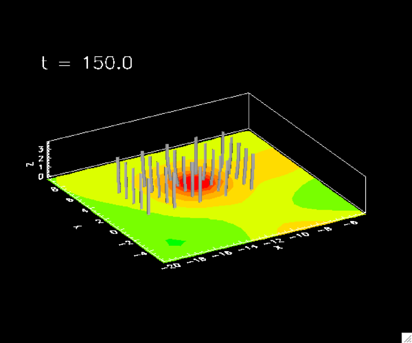
Figure 5: The close up views of the density contours around cores for $\beta_{0}=0.25$. Magnetic field lines near cores are also plotted in three-dimensional space.

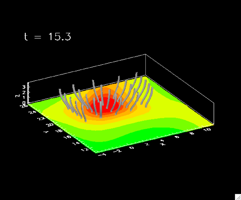
Figure 6: The close up views of the density contours around cores for $\beta_{0}=4$. Magnetic field lines near cores are also plotted in three-dimensional space.

Figure 5 and Figure 6 shows the close up views of the density contours around cores for $\beta_{0}=0.25$ and $\beta_{0}=4$ respectively. Magnetic field lines near cores are also plotted in three-dimensional space. When $\beta_{0}=0.25$, the neutral gas has to slip through the field lines to make a gravitationally bound core. Therefore, the field lines are not so deformed in the case of $\beta_{0}=0.25$, in contrast to those of $\beta_{0}=4$.

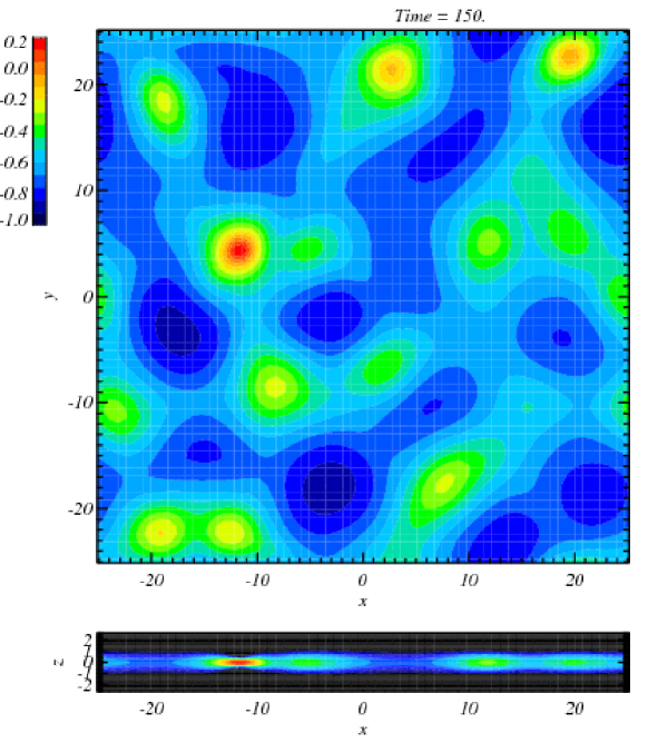
Figure 7: The logarithmic contours of plasma $\beta$ for $\beta_{0}=0.25$ at $t=150$. Upper panel shows the cross section at $z=0$, and the lower panel shows the cross section at $y=4.3$.

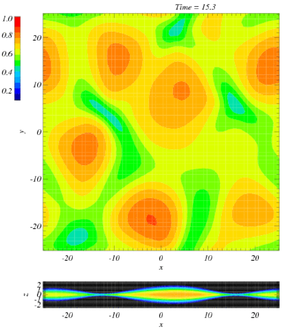
Figure 8: The logarithmic contours of plasma $\beta$ for $\beta_{0}=4$ at $t=15.3$. Upper panel shows the cross section at $z=0$, and the lower panel shows the cross section at $y=5.1$.

Figure 7 and Figure 8 show the logarithmic contours of plasma $\beta$ for $\beta_{0}=0.25$ at $t=150$ and $\beta_{0}=4$ at $t=15.3$, respectively. When $\beta_{0}=0.25$, the plasma $\beta$ in cores is greater than in the surroundings. This is because the mass-to-flux ratio (and therefore $\beta$) has to increase in order for the core to become gravitationally unstable. The maximum $\beta$ is larger than 1 at the centre of a core, which means that the centre of the core is approximately supercritical. In contrast to this, the plasma $\beta$ in cores is slightly lower than the surroundings when $\beta_{0}=4$. In this case, the magnetic field is swept up by the contracting cloud before ion-neutral slip works efficiently. If hydrostatic equilibrium along the $z$-direction is exactly satisfied, the plasma $\beta$ would remain constant in time and space. The slightly lower values of $\beta$ in cores are probably caused by the modestly nonequilibrium state along $z$ during the evolution.

Figure 9: The densities, plasma $\beta$, and $v_{x}$ along $x$-axes for lines that cut through the cores shown in Figure 5 and Figure 6. The left panel shows the core for $\beta_{0}=0.25$. The right panel shows the core for $\beta_{0}=4$.

Figure 10: The densities, plasma $\beta$, and $v_{z}$ along $z$-axes for lines that cut through the cores shown in Figure 5 and Figure 6. The left panel shows the core for $\beta_{0}=0.25$. The right panel shows the core for $\beta_{0}=4$.

Figure 9 shows the densities, plasma $\beta$, and $v_{x}$ along $x$-axes for lines that cut through the cores shown in Figure 5 and Figure 6. The left panel shows the core for $\beta_{0}=0.25$. The right panel shows the core for $\beta_{0}=4$. Figure 9 shows that the plasma $\beta$ in the core is higher than the surroundings for $\beta_{0}=0.25$ and lower for $\beta_{0}=4$. The infall velocity for $\beta_{0}=4$ shows supersonic values, while the velocity for $\beta_{0}=0.25$ is subsonic. These velocities are comparable to those in Figure 2 and Figure 3 of Basu & Ciolek (2004). Figure 10 shows the densities, plasma $\beta$, and $v_{z}$ along $z$-axes for lines that cut through the same cores. It also shows that the infall velocity for $\beta_{0}=4$ reaches mildly supersonic values, while the velocity for $\beta_{0}=0.25$ is subsonic.

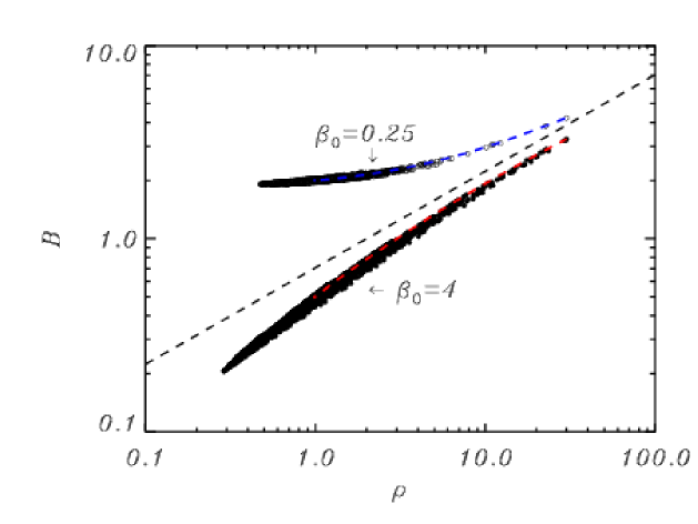
Figure 11: Open circles show the magnetic field strength as a function of density along $z=0$ at $t=150$ for the model with $\beta_{0}=0.25$. The strength of the magnetic field is normalized by $\sqrt{8\pi\rho_{0}c_{s0}^{2}}$. Filled circles are the same for $\beta_{0}=4$, at $t=15.3$. The blue line shows the evolutionary track of the point at which the density achieves its maximum value for the model with $\beta_{0}=0.25$. The red line is the same for $\beta_{0}=4$.

Figure 11 shows the relation between density and magnetic field on the plane $z=0$. The strength of the magnetic field is normalized by $\sqrt{8\pi\rho_{0}c_{s0}^{2}}$. Open circles show the magnetic field strength as a function of density along $z=0$ at $t=150$ for the model with $\beta_{0}=0.25$ (see Fig. 2). Filled circles are the same for $\beta_{0}=4$, at $t=15.3$ (see Fig. 3). The blue line shows the evolutionary track of the point at which the density achieves its maximum value for the model with $\beta_{0}=0.25$. The red line is the same but for $\beta_{0}=4$. This figure shows that the snapshot of the relation between density and magnetic field at different spatial points in the midplane of the cloud overlaps with the evolutionary track of an individual core . The dashed line shows $B\propto\rho^{0.5}$. When the density becomes large, each relation approximately tends to $B\propto\rho^{0.5}$. In the case of $\beta_{0}=0.25$, the relation shows that core initially evolves to greater density without increasing the magnetic field strength. This is caused by the slip of neutral gas through the magnetic field during the subcritical phase of evolution.

4 Conclusions and Discussion

We have studied fragmentation of a sheet-like self-gravitating cloud by three-dimensional MHD simulations. The main results are as follows.

• We confirmed that in the case of an initially subcritical cloud ($\beta_{0}=0.25$), cores developed gradually over an ambipolar diffusion time, while the cores in an initially supercritical cloud ($\beta_{0}=4$ or $\beta_{0}=100$) developed in a dynamical time.

• The infall speed on to cores is subsonic in the case of an initially subcritical cloud, while there is extended supersonic infall in the case of an initially supercritical cloud. This is consistent with the result of the two-dimensional simulations of Basu & Ciolek (2004). In our three-dimensional simulations, we also find that the $z$-component of the velocity follows the same pattern.

• The size of cores for mildly supercritical cloud ($\beta_{0}=4$) is bigger than that of highly supercritical cloud ($\beta_{0}=100$). The size becomes smaller again when the magnetic field is stronger than the critical ($\beta_{0}=0.25$). This result is consistent with the two-dimensional linear analysis of Ciolek & Basu (2006).

• When the cloud is initially subcritical ($\beta_{0}=0.25$), the plasma $\beta$ in cores is greater than in the surroundings. In contrast to this, the plasma $\beta$ in cores is slightly lower than the surroundings when the cloud is initially supercritical ($\beta_{0}=4$). The latter result is probably caused by the modestly nonequilibrium state along $z$ during the evolution.

• In the $B-\rho$ plane, the snapshot of the relation between magnetic field strength ($B$) and density ($\rho$) at different spatial points of the cloud overlaps with the evolutionary track of an individual core. When the density becomes large, each relation approximately tends to $B\propto\rho^{0.5}$.

Our simulation is the first fully three-dimensional simulation to study the role of magnetic fields and ion-neutral friction in fragmentation. In this paper, we concentrated on the effect of initially small perturbations, partly as a way to compare with established predictions of linear theory. Our models also serve as a guide to understand fragmentation occurring exclusively in dense subregions of clouds that contain only subsonic or transonic motions. Real molecular clouds certainly contain supersonic turbulence, at least in their low-density envelopes, as is observed through large line-widths of emission lines from relatively low-density tracers. The additional effect of supersonic turbulence on three-dimensional fragmentation with magnetic fields and ion-neutral friction will be studied in an upcoming paper.

References

- Basu (2000) Basu, S., 2000, ApJ, 540, L103
- Basu (2005) ., 2005, in Chalabaev, A., Montmerle, T., Tran Thanh Van, J., eds, Proc. 39th Rencontres de Moriond, Young Local Universe, Gioi, Hanoi, p. 191
- Basu & Ciolek (2004) Basu, S., Ciolek, G. E., 2004, ApJ, 607, L39
- Basu & Mouschovias (1994) Basu, S., Mouschovias, T. Ch., 1994, ApJ, 432, 720
- Ciolek & Basu (2006) Ciolek, G. E., Basu, S., 2006, ApJ, 652, 442
- Ciolek & Mouschovias (1995) Ciolek, G. E., Mouschovias, T. Ch., 1995, ApJ, 454, 194
- Crutcher (1999) Crutcher, R. M., 1999, ApJ, 520, 706
- Crutcher (2004) ., 2004, ApSS, 292, 225
- Crutcher, Nutter, & Ward-Thompson (2004) Crutcher, R. M., Nutter, D. J., Ward-Thompson, D. W., Kirk, J. M., 2004, ApJ, 600, 279
- Curran et al. (2004) Curran, R. L., Chrysostomou, A., Collett, J. L., Jenness, T., Aitken, D. K., 2004, A&A, 421, 195
- Elmegreen (1979) Elmegreen, B. G., 1979, ApJ, 232, 729
- Indebetouw & Zweibel (2000) Indebetouw, R. M., Zweibel, E. G., 2000, ApJ, 532, 361
- Kirk, Ward-Thompson, & Crutcher (2006) Kirk, J. M., Ward-Thompson, D., Crutcher, R. M., 2006, MNRAS, 369, 144
- Kudoh & Basu (2003) Kudoh, T., Basu. S., 2003, ApJ, 595, 842
- Kudoh & Basu (2006) ., 2006, ApJ, 642, 270
- Kudoh, Matsumoto, & Shibata (1999) Kudoh, T., Matsumoto, R., Shibata, K., 1999, Computational Fluid Dynamics Journal, 8, 56
- Lai et al. (2001) Lai, S.-P., Crutcher, R. M., Girart, J. M., Rao, R., 2001, ApJ, 561, 864
- Lai et al. (2002) ., 2002, ApJ, 566, 925
- Lada & Lada (2003) Lada, C. J., Lada, E. A., 2003, ARAA, 41, 57
- Langer (1978) Langer, W. D., 1978, ApJ, 225, 95
- Li & Nakamura (2004) Li, Z.-Y., Nakamura, F., 2004, ApJ, 609, L83
- McKee (1989) McKee, C. F., 1989, ApJ, 345, 782
- Mestel & Spitzer (1956) Mestel, L., Spitzer, L., Jr., 1956, MNRAS, 116, 503
- Miyama, Narita, & Hayashi (1987a) Miyama, S. M., Narita, S., Hayashi, C., 1987a, Prog. Theor. Phys., 78, 1051
- Miyama, Narita, & Hayashi (1987b) Miyama, S. M., Narita, S., Hayashi, C., 1987b, Prog. Theor. Phys., 78, 1273
- Mouschovias & Spitzer (1976) Mouschovias, T. Ch., Spitzer, L., Jr., 1976, ApJ, 210, 326
- Myers & Goodman (1988) Myers, P. C., Goodman, A. A., 1988, ApJ, 326 L27
- Nakamura & Li (2005) Nakamura, F., Li, Z.-Y., 2005, ApJ, 631, 411
- Nakano (1979) Nakano, T., 1979, PASJ, 31, 697
- Nakano & Nakamura (1978) Nakano, T., Nakamura, T., 1978, PASJ, 30, 671
- Ogata et al. (2004) Ogata, Y., Yabe, T., Shibata, K., Kudoh, T., 2004, International Journal of Computational Methods, 1, 201
- Shu et al. (1999) Shu, F. H., Allen, A., Shang, H., Ostriker, E. C., Li, Z.-Y., 1999, in Lada, C. J., Kylafis, N., eds, The Origin of Stars and Planetary Systems, Kluwer, Dordrecht, p. 193
- Spitzer (1942) Spitzer, L., Jr. 1942, ApJ, 95, 329
- Stone & Norman (1992) Stone, J. M., Norman, M. L., 1992, ApJS, 80, 791
- Strittmatter (1966) Strittmatter, P., 1966, MNRAS, 132, 359
- Tomisaka, Ikeuchi, & Nakamura (1988) Tomisaka, K., Ikeuchi, S., Nakamura, T., 1988, ApJ, 335, 239
- Yabe & Aoki (1991) Yabe, T., Aoki, T., 1991, Comput. Phys. Commun., 66, 219
- Yabe & Wang (1991) Yabe, T., Wang, P.-Y., 1991, J. Phys. Soc. Japan, 60, 2105
- Yabe, Xiao, & Utsumi (2001) Yabe, T., Xiao, F., Utsumi, T., 2001, J. Comput. Phys., 169, 556
- Zweibel (1998) Zweibel, E. G., 1998, ApJ, 499, 746