Chandra ACIS Survey of M33 (ChASeM33): X-ray Imaging Spectroscopy of M33SNR 21, the brightest X-ray Supernova Remnant in M33

Abstract

We present and interpret new X-ray data for M33SNR 21, the brightest X-ray supernova remnant (SNR) in M33. The SNR is in seen projection against (and appears to be interacting with) the bright H ii region NGC 592. Data for this source were obtained as part of the Chandra ACIS Survey of M33 (ChASeM33) Very Large Project. The nearly on-axis Chandra data resolve the SNR into a $\sim 5\arcsec$ diameter (20 pc at our assumed M33 distance of $817\pm 58$ kpc) slightly elliptical shell. The shell is brighter in the east, which suggests that it is encountering higher density material in that direction. The optical emission is coextensive with the X-ray shell in the north, but extends well beyond the X-ray rim in the southwest. Modeling with X-ray spectrum with an absorbed sedov model yields a shock temperature of $0.46^{+0.01}_{-0.02}\,\;\mathrm{keV}$, an ionization timescale of $n_{\mathrm{e}}t=2.1^{+0.2}_{-0.3}\times 10^{12}\,\mathrm{cm}^{-3}\,\mathrm{s}$, and half-solar abundances ($0.45^{+0.12}_{-0.09}$). Assuming Sedov dynamics gives an average preshock H density of $1.7\pm 0.3\,\mathrm{cm}^{-3}$. The dynamical age estimate is $6500\pm 600\,\mathrm{yr}$, while the best fit $n_{\mathit{e}}t$ value and derived $n_{\mathit{e}}$ gives $8200\pm 1700\,\mathrm{yr}$; the weighted mean of the age estimates is $7600\pm 600\,\mathrm{yr}$. We estimate an X-ray luminosity (0.25-4.5 keV) of $(1.2\pm 0.2)\times 10^{37}\,\mathrm{ergs}\,\mathrm{s}^{-1}$ (absorbed), and $(1.7\pm 0.3)\times 10^{37}\,\mathrm{ergs}\,\mathrm{s}^{-1}$ (unabsorbed), in good agreement with the recent XMM-Newton determination. No significant excess hard emission was detected; the luminosity $\leq 1.2\times 10^{35}\,\mathrm{ergs}\,\mathrm{s}^{-1}$ (2-8 keV) for any hard point source.

1 Introduction

Multiwavelength studies of nearby galaxies are becoming increasingly effective at providing statistically interesting samples of many classes of objects, including supernova remnants (SNRs). At a distance of 817$\pm$58 kpc (Freedman et al., 2001) and with a relatively face-on orientation ($i=55\arcdeg\pm 1\arcdeg$; Zaritsky et al., 1989), the late-type Sc spiral galaxy M33 is a key galaxy for such studies. At the assumed distance to M33, 1″ subtends 4$\;\mathrm{pc}$, allowing the morphology of some objects to be studied and many confused or crowded regions to be at least partially resolved, depending on the wavelength band, instrumentation, and available spatial resolution.

Nearly 100 SNRs have been identified in M33, based on a combination of radio and optical imaging and spectroscopy (Dodorico et al., 1978; Sabbadin, 1979; Blair & Kirshner, 1985; Viallefond et al., 1986; Long et al., 1990; Smith et al., 1993; Gordon et al., 1998, 1999). M33 has also been surveyed by each of the imaging X-ray missions, including Einstein (Long et al., 1981a; Trinchieri et al., 1988), ROSAT (Schulman & Bregman, 1995; Long et al., 1996; Haberl & Pietsch, 2001), and XMM-Newton (Pietsch et al., 2003, 2004; Misanovic et al., 2006). The ROSAT survey of Long et al. (1996) found 12 of the 98 optically identified SNRs in the catalog of Gordon et al. (1998, hereafter GKL98), and the XMM-Newton survey of Pietsch et al. (2003, 2004) brought the total number of X-ray SNR identifications to 21. Ghavamian et al. (2005) used archival Chandra data on M33 in comparison with the optical data sets to detect X-ray counterparts to 22 of the 78 GKL98 SNRs within the Chandra fields of view available at that time. Using the characteristics of this X-ray sample, X-ray sources without optical or radio counterparts but with X-ray hardness ratios similar to those of confirmed SNRs were also identified as candidate SNRs. This earlier work was largely responsible for motivating the Chandra ACIS Survey of M33 (ChASeM33), a Very Large Project to examine the X-ray point- and extended-source populations and diffuse X-ray emission in M33 (Sasaki et al., 2007). At this writing, the survey is in progress and nearly complete. Here we choose to highlight observations of a single region in M33 to demonstrate the benefits that this survey will ultimately provide over much of the galaxy.

M33SNR 21 (SNR #21 in the GKL98 catalog; also #121 in Pietsch et al. 2004 and #108 in Misanovic et al. 2006) is the brightest X-ray SNR in M33 and is located in the outskirts of the giant H ii region NGC 592, which is $\sim$9′ due west of the galaxy’s nucleus (see Fig. 1). The relation between the SNR and the H ii region is shown in more detail in Figure 2, an RGB composite image constructed from continuum-subtracted Local Group Galaxy Survey data (LGGS

; Massey et al. 2006), using H$\alpha$ (red), [S ii] (green), and [O iii] (blue) narrow band images; see §3 for further details. The H ii region consists of a pair of bright cores separated by $\sim 25\arcsec$ which are surrounded by extensive ($\sim 2\arcmin\times 2\arcmin$) faint filamentary structure. As indicated, the SNR stands out by virtue of its elevated [S II] emission relative to H$\alpha$, a signature of shock-heated gas (see, e.g., Blair & Long 2004).

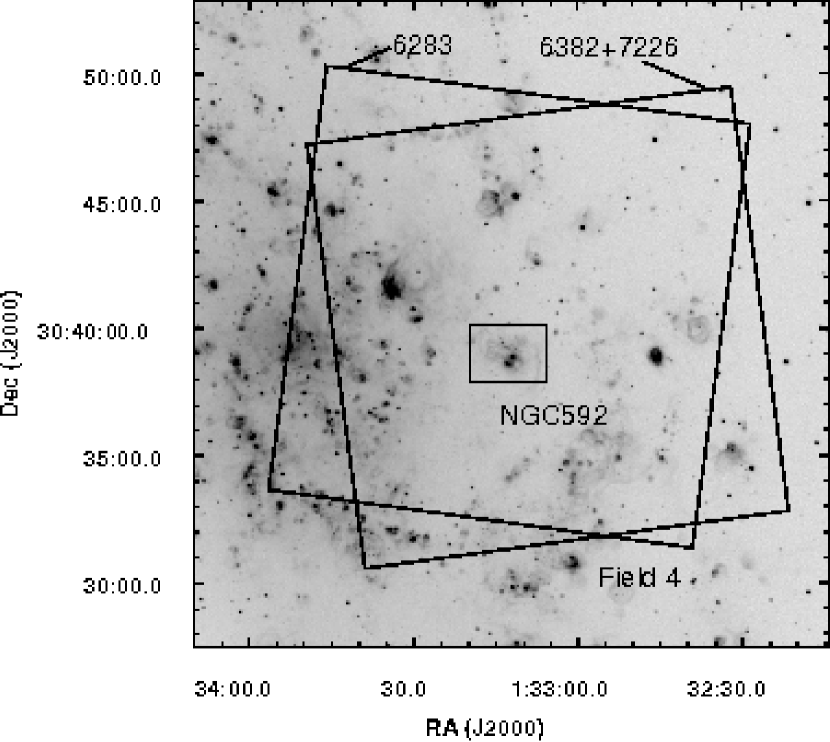
Figure 1: Large squares indicate the $16\farcm 8\times 16\farcm 8$ ACIS-I detector footprint for the pointings closest to the SNR (Field 4), superposed on a deep H$\alpha$ image taken with the Burrell Schmidt telescope at Kitt Peak (McNeil & Winkler, 2006). The small rectangle indicates the region covered by Figure 2

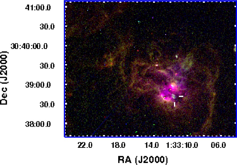
Figure 2: False color RGB composite of continuum-subtracted images from the LGGS of the region surrounding M33SNR 21; H$\alpha$ is shown in red, [S ii] in green, and [O iii] in blue. The SNR appears in projection against the giant H ii region NGC 592. The two bright cores of the H ii region are seen in magenta, and some of the faint outer emission in the northeast can also be seen. M33SNR 21 appears as the indicated cyan structure.

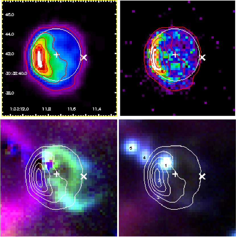
Figure 3: Top left: Exposure-corrected (0.35-4$\;\mathrm{keV}$) Chandra image, binned by 0.5 ACIS pixels in each direction and smoothed with a 3-bin radius Gaussian. The coordinate axes are labeled with J2000 coordinates. The red contours are from a similarly smoothed image for total counts, ranging from 2–18 cts/bin in steps of 4 ct/bin; the background level is 0.03 ct/bin. The white ellipse shows the elliptical shell model dimensions. The central white “+” is the X-ray center, and the white “$\times$” to the west is the centroid position for the nonthermal radio source (see text). Top right: The result of 10 iterations of the Lucy-Richardson deconvolution algorithm. The slight shift of the bright ridge to larger radii is an artifact. Bottom panels: False color RGB composite of the optical images, with H$\alpha$ (red), [S ii] (green), [O iii] (blue). Bottom left: Continuum subtracted LGGS images, overlaid with X-ray contours. Bottom right: LGGS images prior to continuum subtraction, overlaid with X-ray contours. The numbers identify stars from the LGGS catalog (see text).

Long et al. (1981a) first detected M33SNR 21 in X-rays with Einstein, and suggested that it was an SNR based on its extremely soft spectrum. Gordon et al. (1993) confirmed the SNR identification by combining radio (VLA and Westerbork), optical (imaging and spectral), and X-ray (ROSAT) data. The nonthermal nature of the radio emission was important for confirming the SNR in the midst of otherwise thermal emission from the H ii region. Gordon et al. (1993) measured the density-sensitive optical [S ii] lines and found $n_{\mathrm{e}}=270\;\mathrm{cm}^{-3}$, indicating that a dense preshock environment is likely responsible for the high X-ray emissivity. The high luminosity and dense environment are also an indication that the SNR is indeed embedded within the H ii region and not just seen in projection (Gordon et al., 1993). The ROSAT data allowed estimates of $\sim$500 $\rm km~{}s^{-1}$ for the shock velocity and $\sim 4\times 10^{6}\;\mathrm{K}{}$ for the postshock temperature.

More recently, Pietsch et al. (2004) observed M33SNR 21 as part of a deep XMM-Newton survey of M33 and obtained an absorbed 0.2–4.5 keV X-ray flux of $(1.41\pm 0.02)\times 10^{-13}\,\;\mathrm{erg}{}\,\;\mathrm{s}^{-2}\;\mathrm{cm}^{-2}$, which implies an absorbed X-ray luminosity of $(1.13\pm 0.14)\times 10^{37}\,\;\mathrm{erg}{}\,\;\mathrm{s}^{-1}$ at our assumed distance to M33. The SNR has been cataloged and called by a variety of names, including M33 X-3, 2E 0130.3+3023, 013022+30233, 022+233, GKL 21, G98-21, GKL98 21, GDK 29, RX J0133.1+3038, and XMMU J013311.6+303841.

We provide below a detailed analysis of the ChASeM33 data for M33SNR 21. The data reduction and processing steps are described in §2. We select the portion of the data with the best imaging resolution and compare with optical data for the region, finding very different morphologies for the optical and X-ray emitting components of this SNR (§3). We then combine the high resolution X-ray data with other portions of the ChASeM33 data (in which the SNR was farther off-axis) to improve the statistics and perform X-ray spectral analyses (§4). We derive global SNR parameters assuming a Sedov model, and compare and contrast M33SNR 21 with similar SNRs in the LMC – N49 and SNR 0506-68.0 – in §5. The last section, §6, summarizes our results and conclusions.

2 X-ray Observations and Data Reduction

The ChASeM33 survey was designed to cover the inner and most crowded regions of M33 with seven fields, each with a total exposure of 200$\;\mathrm{ks}$ split into two observing intervals; see (Sasaki et al., 2007) for further details on the survey. ACIS-I is the primary detector, while ACIS-S2 and S3 provide additional (though far off-axis) coverage of portions of the galaxy adjacent to the primary positions. At this writing, both $\sim$100$\;\mathrm{ks}$ Field 4 pointings closest to the M33SNR 21 position have been performed (see Fig. 1). The first Field 4 pointing was split into two pieces, ObsIDs 6382 and 7226, totaling 97.2$\;\mathrm{ks}$ after screening for high background. In these data, the SNR is $\sim$1.7′ off-axis on the ACIS-I2 chip and at the same nominal pointing and roll (differing by less than 0.1″ in both); we merged these datasets for subsequent analyses. The second Field 4 pointing, ObsID 6383, was not split and totaled 91.4$\;\mathrm{ks}$ after screening; the SNR was $\sim$2.1′ off-axis on the ACIS-I3 chip. The Field 4 observations are all close enough to on-axis to attain good spatial resolution. We simulated the Chandra PSF with ChaRT (Carter et al., 2003) using the fitted M33SNR 21 spectrum (see §4) and obtained half-power diameters of 0.93″ and 1.01″ for combined ObsIDs 7226+6382 and ObsID 6383, respectively.

M33SNR 21 was also observed in five other pointings at off-axis angles $\sim 8\arcmin$–18′ (see Table 1). Although the rapid degradation of Chandra’s spatial resolution at large off-axis angles (Chandra POG) makes these observations unsuitable for spatial studies of this SNR, the source is bright and isolated enough from other nearby sources to make these data useful for investigating the spectrum of the SNR as a whole. Moreover, ObsIDs 6380 (Field 3) and 6388 (Field 7) imaged the SNR on the ACIS-S3 chip which has superior low-energy response and thus provides improved information about the softest X-rays.

We reprocessed the X-ray data from the Level 1 files to remove pixel randomization and apply time-dependent gain changes. We screened for background flares using the ACIS-I3 light curves except for the ACIS-S3 data, for which we used the ACIS-S3 light curves. We used CIAO version 3.3.0.1 and CALDB version 3.2.0. In the Field 4 ObsIDs 6282 and 7226, the source dithered across two ACIS I2 “bad” columns (162, 196), resulting in the loss of $\sim 13$% of the counts from the SNR. These columns had been marked bad because of a slight excess background. However, the SNR spans only a short stretch of the columns, and a careful examination of the rest of the data for these columns showed that the spurious background would be negligible for the SNR extraction region ($\sim 0.3$ ct for column 162, effectively 0 for column 196). Accordingly, we restored those columns for the analysis to improve the statistics. All the Field 4 data were merged for the imaging analysis to improve the statistics. We applied a subpixel event repositioning (SER) correction to the data using software developed by Li et al. (2004, software available from the Chandra contributed software page) to improve the spatial resolution. The SER algorithm uses the distribution of pulse height amplitudes (PHAs) within the $3\times 3$ pixel event islands to improve the event centroiding.

From the processed event list, we construct a 0.35–4$\;\mathrm{keV}$ “total counts” image (ct/bin) by binning the events from the merged $\sim 200\;\mathrm{ks}{}$ Field 4 data set by 1/2 ACIS pixel in each direction ($\sim 1/4\arcsec\times 1/4\arcsec$ bins). We divide this counts image by a corresponding exposure map constructed using the fitted SNR spectrum (see §4) to generate an exposure corrected image ($\mathrm{phot}\,\mathrm{cm}^{-2}\,\mathrm{s}^{-1}$). This exposure-corrected image is then smoothed with a 3 bin radius Gaussian kernel. The image was overlaid by contours from a similarly smoothed version of the original total counts image, with contours ranging from 2 ct/bin to 18 ct/bin at intervals of 4 ct/bin. The corresponding background level is $\sim 0.03$ ct/bin. The processed X-ray imaging data are shown and compared with optical images of the region in Figure 3; see §3 for a discussion of the optical data. The upper left panel of Figure 3 shows the smoothed, exposure-corrected 0.35–4$\;\mathrm{keV}$ image from the combined $\sim 200\;\mathrm{ks}{}$ Field 4 data set, binned to 1/2 ACIS pixel in each direction, with contours from the smoothed total counts image as described above. The X-ray imagery reveals a strong asymmetry in the surface brightness distribution. The bright clump in the east has a surface brightness $\sim 5$ times that of the fainter portions of the SNR. To examine potential finer spatial structure of M33SNR 21, we experimented with Lucy-Richardson deconvolutions of this image. The upper right panel of Figure 3 shows the result for 10 iterations with the CIAO tool arestore using the combined Field 4 (ObsIDs 6382, 7226, and 6383) total counts image, and merged ChaRT simulations for the PSF. The deconvolution shows an arc of bright emission in the east, and possibly some patchy structure within the interior. The slight shift of the bright ridge to larger radii is an artifact of the reconstruction.

Table 1: Chandra X-Ray Observations

Field	Obsids	$\theta$	Exp	CCD	Counts
		(arcmin)	$(\;\mathrm{ks})$		(0.35–4$\;\mathrm{keV}$)
4	7226, 6382	1.66	97.2	I2	1850
	6383	2.06	91.4	I3	1740
5	6184, 7170, 7171	7.77	100.1	I0	1470
1	6376	8.51	93.1	I1	1430
3	6380	11.26	89.7	S3	2155
2	6378	16.21	103.7	S2	1746
7	6388	17.60	88.7	S3	2470

Figure 4: Elliptical shell fit to Field 4 image data. The panels compare the data and projected model for the four quadrants centered on North, South, East, and West.

3 Imaging Analysis

For optical images of the M33SNR 21 field, we took data from the Local Group Galaxies Survey (LGGS; Massey et al. 2006) which used the KPNO 4m telescope and Mosaic CCD camera to survey most of M33 (3 overlapping fields) through narrow-band H$\alpha$, [O iii] $\lambda$ 5007, and [S ii] $\lambda\lambda 6716,6731$ filters, plus broadband UBVRI. M33SNR 21 appears in both the north and central fields. From each Mosaic image we clipped out a small section centered on the SNR and precisely aligned these using several dozen field stars. We then selected the images with the best seeing in each of the 3 emission lines (all from the north field) and in the V and R bands (both from the central field) and matched the point-spread functions. Finally we scaled the broadband images appropriately, and performed continuum subtraction to remove the stars as effectively as possible. In this case, we subtracted V from [O iii], and R from both H$\alpha$ and [S ii]. The result is shown in Figure 2. The lower left panel of Figure 3 is an enlarged version of the same image with colors rescaled to emphasize the SNR, and the lower right panel is an RGB composite of the narrow-band images prior to continuum subtraction to show the locations of the bright stars. X-ray contours have been plotted on both to facilitate comparison with the upper panels. Based on the V magnitudes and UBVRI colors obtained by the LGGS, the three stars seen in projection (labeled “1”, “2”, and “3”) and the star furthest to the northeast (“5”) are O stars in M33. Typical O star X-ray luminosities are $\lesssim 10^{33}\;\mathrm{erg}{}\,\;\mathrm{s}^{-1}$ (Vaiana et al., 1981) and an O star would be undetectable in the 500$\;\mathrm{ks}$ of data used in our analysis. The “star” closest to the northeast rim , “4”, consists of three stars, two of which appear to be O stars. The third (much fainter) star has an unusual color, but no X-ray events were detected in the 190$\;\mathrm{ks}$ of the Field 4 imaging data (Fig. 3). The X-ray data are not significantly contaminated by stellar emission.

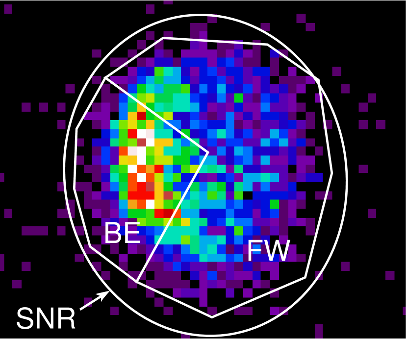
Figure 5: Unsmoothed total counts image, binned to 1/2 ACIS pixels. The Field 4 Bright Eastern (“BE”) and Faint Western (“FW”) wedge extraction regions are indicated. The extraction region for the full SNR is indicated by the ellipse labeled “SNR”.

To characterize the overall shape of the X-ray SNR, we fitted the 0.35-4$\;\mathrm{keV}$ image data with an elliptical shell model (assuming that the symmetry axis lies in the plane of the sky), with density within the shell varying azimuthally as

$$n(\theta)\propto n_{0}(1+0.5A(1+\cos(\theta-\theta_{0}))).$$ (1)

Figure 4 shows four projections of the model onto the data (including the effect of the simulated Chandra PSF) for quadrants centered on north, south, east, and west. The greater brightness in the eastern quadrant compared to the western quadrant is evident. The model shows the SNR to be slightly elliptical (axis ratio 1.07) with the position angle of the major axis $\sim 9^{\circ}$ east from north. The semimajor (semiminor) axis is 2.65″(2.48″) with an uncertainty of $\sim\pm 0.05\arcsec$. At the assumed distance of M33, this corresponds to a semimajor (semiminor) axis of 10.5$\;\mathrm{pc}$ (9.8$\;\mathrm{pc}$) with an uncertainty of $\sim\pm 0.2\,\mathrm{pc}$, and an overall size uncertainty of $\sim 0.7\,\mathrm{pc}$ when the distance uncertainty is included. The surface brightness peaks at position angle $\sim 104\arcdeg$ east from north. The fitted value for the factor $A$ in the elliptical shell model is 1.19; this implies the ambient density on the bright side is about a factor of $1+A\approx 2$ higher than that on the faint side. The outline of the elliptical shell model is indicated by an ellipse in the upper panels of Figure 3. Compared to the fitted ellipse, the X-ray emission extends slightly further to the south than other directions (Fig. 3, upper left panel; see also the comparison between the northern vs. southern quadrants in Figure 4). The fractional thickness of the shell, $\Delta R_{\mathit{s}}/R_{\mathit{s}}$, is poorly constrained because the SNR is only barely resolved; we found that a value of $0.065$ provides an adequate description for the limb-brightening of the SNR’s shell. The resulting center position is $(\alpha_{\mathrm{J2000}},\delta_{\mathrm{J2000}})$=($01^{\mathrm{h}}33^{\mathrm{m}}11\fs 73$, +$30\arcdeg 38\arcmin 41\farcs 9$), indicated by the central “+” in each panel of Figure 3. This position agrees well with the XMM-Newton position determination (Misanovic et al., 2006) of $(\alpha_{\mathrm{J2000}},\delta_{\mathrm{J2000}})=(01^{\mathrm{h}}33^{\mathrm{m}}11\fs 76$, +$30\arcdeg 38\arcmin 42\farcs 1)$, well within the XMM-Newton uncertainty of 0.55″.

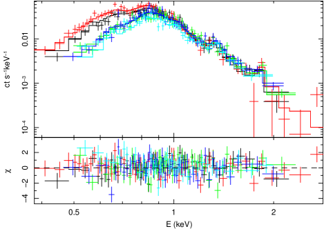
Figure 6: Chandra ACIS-I and ACIS-S3 spectra and best fit sedov model of M33SNR 21; the curves which are higher at low energies are ACIS-S3, and the rest are ACIS-I data.

Using techniques similar to those in the Weisskopf & Hughes (2006) review paper, we also examined the merged Field 4 hard band (3–8$\;\mathrm{keV}$) image for any indications of a point source or emission from a plerion. The extraction region for the whole SNR includes only 14 counts in the 3–8$\;\mathrm{keV}$ band during the entire 190 ks integration. The best fit XSPEC sedov model (see §4) predicts $11\pm 5$ counts in this band, so there is no evidence for a significant excess of hard emission. The brightest potential point source has a total of 3 counts (3–8$\;\mathrm{keV}$) within two adjacent pixels, providing a 3$\sigma$ count rate upper limit of $\lesssim 4.2\times 10^{-5}\,\mathrm{ct}\,\mathrm{s}^{-1}$. If we assume a Crab-like powerlaw spectrum (powerlaw index $\alpha=2.05$), the same absorbing column as for the best fit sedov model and the response for the ACIS-I2 observation, this count rate limit allows an unabsorbed flux upper limit for a point source of $\lesssim 1.5\times 10^{-15}\,\mathrm{erg}\,\mathrm{cm}^{-2}\,\mathrm{s}^{-1}$ (2–8 $\;\mathrm{keV}$) corresponding to an unabsorbed X-ray luminosity upper limit of $\lesssim 1.2\times 10^{35}\,\mathrm{erg}\,\mathrm{s}^{-1}$ for the same band.

The centroid of the nonthermal radio source (Gordon et al., 1993, precessed to J2000) is 2.8″ west of the center of the X-ray emission, and indicated by a “$\times$” toward the right in each panel of Figure 3. Thermal emission from the H ii region may confuse the radio picture (Gordon et al., 1993). The resolution of the radio data is $\sim 7\arcsec$ so the $\sim 3\arcsec$ offset of the radio centroid from the X-ray center is unlikely to be significant.

The relative morphologies of the optical and X-ray emissions from M33SNR 21 are interesting and somewhat perplexing. The X-ray SNR appears nearly circular, although with the strong brightness gradient already described, but the optical SNR appears somewhat more structured and extended. The bright optical emission agrees well with the outer X-ray contour shown in Figure 3 along the northern and northwestern X-ray limbs, apparently validating the relative astrometry used to align the images. However, the bright eastern X-ray limb is almost devoid of optical emission (although this comparison is hampered by the stellar emission) and faint optical emission extends farther to the southwest from the X-ray contour. Taken on its own, the optical morphology in the southwest is reminiscent of a “blow-out,” which is consistent with the idea that the density is lower on the side of the SNR away from the bright H ii cores. The absence of optical emission on the eastern X-ray peak does not appear to be due to obscuration, as the $N_{\mathrm{H}}$ column derived below is not extreme.

Table 2: Spectral Fit Results for M33SNR 21.

Parameter	Units	BE	FW	SNR	SNR
		F4 data	F4 data	F4 data	F1,3,4,7 data
const(phabs(vphabs(pshock))) model
Abundance	(solar)	$\displaystyle 0.4^{+0.6}_{-0.2}$	$\displaystyle 0.4^{+0.3}_{-0.1}$	$\displaystyle 0.3\pm 0.1$	$\displaystyle 0.28^{+0.06}_{-0.05}$
$kT_{\mathit{e}}$	[keV]	$\displaystyle 0.55^{+0.04}_{-0.07}$	$\displaystyle 0.61^{+0.04}_{-0.05}$	$\displaystyle 0.58\pm 0.03$	$\displaystyle 0.58\pm 0.02$
$\tau$	[10${}^{12}\,\;\mathrm{cm}^{-3}\,\sec$]	$\displaystyle 0.7^{+0.4}_{-0.2}$	$\displaystyle 0.8^{+0.5}_{-0.3}$	$\displaystyle 0.8^{+0.3}_{-0.2}$	$\displaystyle 0.6\pm 0.1$
$N_{\rm H,M33}$	[10${}^{20}\,\;\mathrm{cm}^{-2}$]	$\displaystyle\leq 7.8$	$\displaystyle 2.4^{+14.3}_{-2.0}$	$\displaystyle\leq 3.0$	$\displaystyle\leq 2.9$
$K$	[$10^{-4}\;\mathrm{cm}^{-5}$]	$\displaystyle 0.54\pm 0.02$	$\displaystyle 0.61^{+0.03}_{-0.02}$	$\displaystyle 1.36^{+0.03}_{-0.04}$	$\displaystyle 1.46^{+0.03}_{-0.02}$
$\chi^{2}_{\mathit{red}}$ (d.o.f.)		$\displaystyle 1.11(51)$	$\displaystyle 1.11(62)$	$\displaystyle 1.14(111)$	$\displaystyle 1.14(259)$
const(phabs(vphabs(sedov))) model
Abundance	(solar)	$\displaystyle 0.5^{+0.6}_{-0.2}$	$\displaystyle 0.7^{+2.1}_{-0.3}$	$\displaystyle 0.5^{+0.3}_{-0.2}$	$\displaystyle 0.45^{+0.12}_{-0.09}$
$kT_{\mathit{e}}$	[keV]	$\displaystyle 0.43^{+0.03}_{-0.05}$	$\displaystyle 0.48^{+0.04}_{-0.08}$	$\displaystyle 0.46\pm 0.02$	$\displaystyle 0.46^{+0.01}_{-0.02}$
$\tau$	[10${}^{12}\,\;\mathrm{cm}^{-3}\,\sec$]	$\displaystyle 2.4^{+1.5}_{-0.8}$	$\displaystyle 2.4^{+1.7}_{-1.2}$	$\displaystyle 2.6^{+0.9}_{-0.6}$	$\displaystyle 2.1^{+0.2}_{-0.3}$
$N_{\rm H,M33}$	[10${}^{20}\,\;\mathrm{cm}^{-2}$]	$\displaystyle\leq 9.6$	$\displaystyle 4.1^{+17.5}_{-4.1}$	$\displaystyle\leq 4.0$	$\displaystyle\leq 3.4$
$K$	[$10^{-4}\,\;\mathrm{cm}^{-5}$]	$\displaystyle 0.51\pm 0.02$	$\displaystyle 0.49\pm 0.02$	$\displaystyle 1.08\pm 0.03$	$\displaystyle 1.20\pm 0.02$
$\chi^{2}_{\mathit{red}}$ (d.o.f.)		$\displaystyle 1.02(51)$	$\displaystyle 1.05(62)$	$\displaystyle 1.07(111)$	$\displaystyle 1.08(261)$

Note. — Error ranges are 90% confidence intervals ($\Delta\chi^{2}\leq 2.706$ for one parameter).

Table 3: X-ray fluxes and luminosities based on the sedov model fits

Band	$F$ (absorbed)	$F$ (unabsorbed)	$L_{X}$ (absorbed)	$L_{X}$ (unabsorbed)
	$(10^{-13}\,\;\mathrm{erg}\,\mathrm{s}^{-1}\,\;\mathrm{cm}^{-2})$	$(10^{-13}\,\;\mathrm{erg}\,\mathrm{s}^{-1}\,\;\mathrm{cm}^{-2})$	$(10^{37}\,\;\mathrm{erg}\,\mathrm{s}^{-1})$	$(10^{37}\,\;\mathrm{erg}\,\mathrm{s}^{-1})$
0.35–3.0 $\;\mathrm{keV}$	$1.46\pm 0.03$	$1.95\pm 0.03$	$1.2\pm 0.2$	$1.6\pm 0.3$
0.245–4.5 $\;\mathrm{keV}$	$1.50\pm 0.03$	$2.15\pm 0.04$	$1.2\pm 0.2$	$1.7\pm 0.3$

4 Spectral Analyses

The combined Field 4 data (the only X-ray data for which the SNR is resolved well enough to extract spectra from individual subregions) has $\sim 3600$ counts. We extracted spectra from two wedge-shaped regions, each containing roughly half the total counts: the bright eastern part (“BE”, $\sim 1600$ counts), and the fainter western part (“FW”, $\sim 2000$ counts); see Figure 5. The BE region has $28$% of the area. We also extracted spectra for the SNR as a whole using an elliptical region (“SNR”; see Figure 5). Because ObsIDs 6382 and 7226 fell on the ACIS-I2 chip, while ObsID 6383 fell on ACIS-I3, we extracted separate spectra for the merged 6382+7226 data and the 6383 data. The data were grouped to a minimum of 25 counts/bin, and the $\chi^{2}$ statistic was used for the fits. Background spectra were extracted from larger adjacent regions. In order to improve the fit statistics for the spectrum for the SNR as a whole, we also extracted spectra for a number of the far off-axis observations: Field 1 (ACIS-I1), and Fields 3 and 7 (ACIS-S3). The source and background extraction regions were enlarged appropriately to account for the expansion of the Chandra PSF at large off-axis angles. This provided a total of $\sim 10000$ counts for the SNR as a whole. For the ACIS-S3 data (Fields 3 and 7), the SNR was imaged near the edge of the chip and $\sim 10\%$ of the flux spilled off the chip.

We fitted the spectra using XSPEC version 11.3.2. In each case, we included absorption (phabs) corresponding to a Galactic column of $N_{\mathrm{H}}=5.5\times 10^{20}\,\;\mathrm{cm}^{-2}$ toward M33 (Stark et al., 1995); this component was frozen during the fits. To account for absorption within M33, we included a second absorption component (vphabs) which was allowed to vary: the abundances of the vphabs component were fixed to be 0.5 solar, where we assume Anders & Grevesse (1989) values for the solar abundance set. The M33 abundance at the galactocentric radius of M33SNR 21 is $\sim 0.5\,Z_{\odot}$ (Henry & Howard, 1995). For the thermal component, we examined collisional ionization equilibrium models (which provided very poor fits), and a number of nonequilibrium ionization (NEI) models: nei, pshock, and sedov. The nei and pshock models represent impulsive heating to a constant temperature, $T$; in the former model, the spectrum evaluated at a single ionization timescale, $\tau\equiv n_{\mathit{e}}t$, while in the latter, the spectrum is integrated over ionization timescales from $\tau=0$ to $n_{\mathit{e}}t$. In the sedov model, the nonequilibrium ionization spectrum is integrated over a Sedov-stage SNR profile, and the ionization timescale is $\tau=n_{\mathit{e,s}}\,t_{0}$ where $n_{\mathit{e,s}}$ is the postshock electron density and $t_{0}$ is the age of the SNR. See Borkowski et al. (2001) for a more detailed description of the models.

We performed fits for regions BE, FW, and the whole SNR using the high spatial resolution Field 4 data, and also for the whole SNR including data from Fields 1, 3, and 7 in addition to Field 4. The spectra were fitted simultaneously with the model parameters (including model normalizations) linked. To account for the loss of flux off the chip for the ACIS-S3 data, an additional multiplicative const model was applied, allowed to be free for the ACIS-S3 datasets, and fixed at 1.0 for the other datasets. The resulting const fit values were $\sim 0.9$ for the ACIS-S3 data, as expected.

All three models had comparable $\chi^{2}_{\mathit{red}}\sim 1$, but the sedov models consistently produced better fits: 1.08 for 261 degrees of freedom (dof) for sedov vs. 1.14 (259 dof) and 1.21 (259 dof) for pshock and nei, respectively. The nei and pshock models gave lower abundance estimates ($0.15$–$0.19Z_{\odot}$ and $0.22$–$0.34Z_{\odot}$, respectively) compared to the sedov model ($0.36$–$0.57Z_{\odot}$). The temperatures were $0.52$–$0.56\;\mathrm{keV}{}$ (nei), $0.56$–$0.6\;\mathrm{keV}{}$ (pshock), and $0.44$–$0.47\;\mathrm{keV}{}$ (sedov). The pshock and sedov fit parameters are listed in Table 2; the listed parameter uncertainties are 90% confidence intervals ($\Delta\chi^{2}\leq 2.706$ for one parameter) based on the statistical errors.

In the sedov model, the temperature parameter is the postshock (electron) temperature. In the Sedov self-similar solution the temperature increases (and the density decreases) radially inwards so that the emission-weighted X-ray temperature is $\sim 1.3$ times the shock temperature (Rappaport et al., 1974). In the other two models, nei and pshock, the temperature parameter is the (constant) postshock temperature. If the temperature in the SNR is in fact increasing radially inwards as in the Sedov solution, the fitted temperature parameters for the nei and pshock models would reflect an average X-ray temperature higher than the temperature at the shock front; this would be consistent with the generally higher temperature parameters in those fits compared to the sedov model fits (Table 2).

Based on the best fitting sedov model, we evaluated the X-ray flux and luminosity (absorbed and unabsorbed) for 0.35–3 $\;\mathrm{keV}$ (the range best constrained by the data) and a broader 0.25–4.5 $\;\mathrm{keV}$ range; the results are presented in Table 3. The quoted errors include the normalization uncertainty (Table 2) and the distance uncertainty. These luminosities may be compared to the luminosities (scaled to 817$\;\mathrm{kpc}$) estimated with Einstein IPC ($1.7\times 10^{37}\,\mathrm{erg}\,\mathrm{s}^{-1}$ absorbed, 0.15–4.5 keV; Long et al. 1981a), ROSAT PSPC (flux $1.4\times 10^{-13}\,\mathrm{erg}\,\mathrm{cm}^{-2}\,\mathrm{s}^{-1}$ implying $L_{X}=1.1\times 10^{37}\,\mathrm{erg}\,\mathrm{s}^{-1}$ absorbed, 0.1–2.4 keV; Haberl & Pietsch 2001) and XMM-Newton EPIC (flux $(1.41\pm 0.02)\times 10^{-13}\,\mathrm{erg}\,\mathrm{cm}^{-2}\,\mathrm{s}^{-1}$ implying $L_{\mathit{X}}=(1.13\pm 0.16)\times 10^{37}\,\mathrm{erg}\,\mathrm{s}^{-1}$ absorbed, 0.2–4.5 keV; Pietsch et al. 2004). Our luminosity estimate of $L_{\mathit{X}}=(1.2\pm 0.2)\times 10^{37}\,\mathrm{erg}\,\mathrm{s}^{-1}$ (absorbed, 0.25–4.5 keV) is in good agreement with the ROSAT and XMM-Newton estimates and in reasonable agreement with the Einstein estimate. It is also worth noting that the SNR X-ray luminosity function for M33 does not reach as high as in other nearby galaxies (Ghavamian et al., 2005). M33SNR 21, the brightest SNR in M33, would be only the fourth or fifth brightest SNR if it were in the Large Magellanic Cloud (LMC), based on the luminosities reported in Long et al. (1981b).

5 Discussion

5.1 Association with NGC 592

As noted in §1, the SNR lies along the line of sight to the bright H ii region NGC 592. The high X-ray luminosity of the SNR and the relatively high density interstellar medium (ISM) inferred from the optical [S ii] emission imply that the SNR is in fact embedded in the H ii region (Gordon et al., 1993). The fact that the X-ray emission from M33SNR 21 is brightest on the side toward the bright H ii region core further supports the association with NGC 592. This suggests that the M33SNR 21 progenitor could have been a massive star associated with the burst of star formation which produced NGC 592.

Pellerin (2006) recently reported on FUSE observations of NGC 592 in which the FUSE 30″ aperture covered the bright H$\alpha$ cores (but excluded M33SNR 21). The line profiles show extended blue absorption wings, indicating the presence of evolved O stars. Her fits to synthetic spectra based on stellar population models are consistent with a $4.0\pm 0.5$ Myr population at solar metallicity; the FUV models are consistent with a range of $\sim 0.4$–1.2 solar. Bosch et al. (2002) estimated a population age of $\gtrsim 4.5$ Myr, but Pellerin argues that this is inconsistent with the strength of the P-Cygni features. If we assume that the M33SNR 21 progenitor belongs to the same population, the models of Maeder (1990) suggest an initial stellar mass of $\sim 50\,M_{\odot}$ for half-solar to solar abundances. Our X-ray spectroscopic analysis of M33SNR 21 with Chandra data also suggests roughly half-solar abundances. The lack of an X-ray signature from ejecta is likely a combination of the age of the SNR ($\sim 5$–10 kyr) and the limited Chandra spatial resolution at the distance of M33. For the integrated spectrum for the SNR as a whole, most of the X-ray emission arises from the swept-up interstellar medium in M33. These high spatial resolution X-ray observations apparently do not provide sufficient resolution and statistics to separate out high abundance clumps if they are present.

Pellerin (2006) also obtained an intrinsic extinction of $E(B-V)_{i}=0.07\pm 0.02$ for the H ii region. For this extinction, the LMC interstellar extinction curve (Fitzpatrick, 1986) implies $N_{\mathrm{H}}\approx 1.7\times 10^{21}\,\;\mathrm{cm}^{-2}$, while the Galactic extinction curve (Bohlin et al., 1978) implies $N_{\mathrm{H}}\approx 4\times 10^{20}\,\;\mathrm{cm}^{-2}$. The analysis of the Chandra X-ray spectra provides primarily upper limits $N_{\mathrm{H}}\leq(2$–10$)\times 10^{20}\,\;\mathrm{cm}^{-2}$ for the M33 column, consistent with a solar metallicity extinction curve. However, given the complex environment, the position of M33SNR 21 along the line of sight to NGC 592 cannot be determined at present. If the SNR is toward the near side of the H ii region, the low column for the X-ray data could also be consistent with the FUV data and a half-solar metallicity extinction curve.

5.2 Sedov Analysis

In the following, we examine the global properties of M33SNR 21 based on the assumption of a Sedov-stage SNR. Hnatyk & Petruk (1999) investigated the properties of nonspherical SNRs using approximate analytic models, including the cases of an SNR in an exponential density gradient, and an SNR in an off-center $r^{-2}$ powerlaw distribution (for example, an explosion in the wind cavity of another star). The integrated spectral properties of the SNRs were found to be approximately like those of Sedov models, even though the detailed properties are expected to vary spatially across the SNRs. The surface brightness ($\propto n^{2}$) varies more strongly with density around the remnant than the temperature ($\propto n$), and the shock velocity varies only weakly ($\propto n^{1/2}$). The properties derived from the sedov model fits should represent values averaged over the SNR.

The Sedov solution depends on three parameters: the explosion energy, $E_{0}$, the ambient mass density, $\rho_{0}$, and the time since the explosion, $t_{0}$. The ambient density of hydrogen, $n_{0}$, is related to the mass density by $n_{0}=\rho_{0}/(1.43\,\mathrm{amu})$, where we assume a fully ionized gas with half-solar abundances (based on the Anders & Grevesse 1989 solar abundance set). The XSPEC sedov model fits provide estimates for the postshock temperature, $T_{\mathit{s}}$, the ionization timescale, $\tau\equiv n_{\mathit{e,s}}t_{0}$, and also a model normalization $K=(10^{-14}/(4\pi D^{2}))\int\,dV\,n_{\mathit{e}}\,n_{\mathrm{H}}$. In the ionization timescale, $n_{\mathit{e,s}}$ is the postshock electron number density (where we are assuming electron-ion equilibration in the shock), and $n_{\mathit{e,s}}\approx 4.8\times n_{0}$ for our assumed abundances, and assuming strong shock jump conditions. For M33SNR 21, we also have an estimate for the physical radius of the SNR, $R_{\mathit{s}}$, based on the angular radius, $\theta_{\mathit{s}}$, and the distance to M33. With four observational constraints and three model parameters, the system is overconstrained. As noted by Hughes et al. (1998), the age estimates based on the Sedov dynamical age and the age based on ionization timescale allow for a consistency check. If the SNR is well modeled by a Sedov solution, these two age estimates should be the consistent with each other.

The X-ray temperature implies a shock velocity,

$$v_{\mathit{s}}=\left({16kT_{\mathit{s}}\over 3\mu_{\mathit{s}}}\right)^{1/2}=904\,T_{\mathit{s},\mathrm{keV}}^{1/2}\,\;\mathrm{km}\;\mathrm{s}^{-1}{}$$ (2)

where $kT_{\mathit{s},\mathrm{keV}}$ is the postshock temperature in $\;\mathrm{keV}$ and $\mu_{\mathit{s}}$ is the postshock mean mass per free particle. The equation assumes a strong shock into a monatomic gas with three degrees of freedom, and complete equilibration between species (McKee & Hollenbach, 1980). For a fully ionized plasma with half-solar abundances, $\mu_{\mathit{s}}=(m_{\mathrm{H}}+A_{\mathrm{He}}m_{\mathrm{He}}+\cdots)/(2+3A_{\mathrm{He}}+\cdots)\approx 0.61$, where $m_{\mathit{H}}$ and $m_{\mathit{He}}$ are the atomic weights of H and He, respectively, and $A_{\mathrm{He}}$ is the fractional abundance of He relative to H. From the sedov model estimate for the postshock temperature, we have $v_{\mathit{s}}=611\pm 12\;\mathrm{km}\;\mathrm{s}^{-1}{}$ where the error is a purely statistical error, and almost certainly underestimates the real uncertainty in the velocity.

If the SNR is assumed to be expanding as $R_{\mathit{s}}\propto t^{\delta}$, the shock velocity, combined with the current SNR radius, allows for an estimate of the SNR dynamical age, $t_{0}$. The model normalization, $K$, combined with $v_{\mathit{s}}$, provides an estimate for the ambient hydrogen density, $n_{0}$, and the postshock electron density, $n_{\mathit{e,s}}=4.8\,n_{0}$, can be estimated by using the strong shock jump conditions and the (half-solar) abundances. The postshock density can be combined with the ionization timescale estimate, $\tau$, from the sedov model fit to provide a second estimate for the SNR age. From these basic parameters, the swept up mass, $M_{\mathit{SU}}$, and the explosion energy, $E_{0}$, can be estimated. We proceed to the evaluation of the parameters based on the sedov fit parameters from simultaneous fits to the data for the whole SNR (the right hand column in Table 2).

The mean angular radius of the X-ray SNR is $2.56\arcsec\pm 0.13\arcsec$, where the uncertainty in the radius includes a 2% angular size uncertainty and 3.5% uncertainty (added in quadrature) for the azimuthal asymmetry. This angular radius and the assumed distance to M33 imply a radius of $10.1\pm 0.9\;\mathrm{pc}{}$ for the SNR, where the distance uncertainty is now included. For a Sedov-stage SNR, the deceleration parameter is $\delta=2/5$, and we estimate the dynamical age to be $(2/5)R_{\mathit{s}}/v_{\mathit{s}}\approx 6500\pm 600\,\mathrm{yr}$. Given the radial dependence of the electron and H number densities, the emission integral, $\int\,dV\,n_{\mathit{e}}\,n_{\mathrm{H}}$, can be evaluated from the model normalization. For the case of the Sedov solution,

$$\int\,dV\,n_{\mathit{e}}\,n_{\mathrm{H}}\approx 4\xi\left({n_{\mathit{e}}\over n_{\mathrm{H}}}\right)n_{0}^{2}\left({4\pi\over 3}R_{\mathit{s}}^{3}\right)$$ (3)

where $n_{0}$ is the preshock H density and $\xi=0.517773$ is an integration constant evaluated by numerical integration over the Sedov solution. The average preshock H density can be estimated as

$$n_{0}=1.58\,K^{1/2}_{-4}\,D_{800}\,R_{\mathit{s,10}}^{-3/2}\,\;\mathrm{cm}^{-3},$$ (4)

where $K_{-4}$ is the XSPEC sedov model normalization in units of $10^{-4}\;\mathrm{cm}^{-5}$, $D_{800}$ is the distance to the SNR in units of 800$\;\mathrm{kpc}$, and $R_{\mathit{s,10}}$ is the radius of the SNR in units of 10$\;\mathrm{pc}$. From the sedov fit parameters, we obtain an average preshock H density of $n_{0}=1.7\pm 0.3\,\;\mathrm{cm}^{-3}$. Approximate pressure equilibrium around the rim of the SNR would imply that the temperature should vary as $\sim n_{0}^{-1}$. Although the temperature derived from the fit to the BE region is somewhat higher than that obtained from the FW region fit (though not significantly so), even taking the full 90% confidence ranges into account does not provide the $\sim 2$:1 ratio implied by the density variation from the elliptical shell model fit (see §3). The relative overpressure of the BE region compared to the FW region may be an indication that the encounter with the density gradient toward the east is relatively recent. This might also explain the lack of optical emission (see §3) if there has not been sufficient time for the shocks to become radiative. In principle, the ionization timescale provides a constraint on the age of the encounter; however, 90% confidence intervals for $\tau$ for the BE and FW regions are broad enough to make this a weak constraint. An additional possibility is that there are sufficient photoionizing photons toward the east to prevent the postshock gas from recombining. It is notable that the edge of the enhanced [S ii] in the east coincides roughly with a bright rim of H$\alpha$ emission associated with one of the bright cores of the H ii region.

If a Sedov-stage SNR is assumed, the ionization timescale provides for another estimate for the SNR age: $t_{0}=\tau/n_{\mathit{e,s}}\approx 8200\pm 1700\,\mathrm{yr}$. The age based on ionization timescale is somewhat larger than the dynamical age, but the estimates are reasonably consistent. The weighted mean of the estimates yields an age of $6700\pm 600\,\mathrm{yr}$.

From the preshock H density and the radius of the SNR, the swept up mass is $\sim 260\pm 80\,M_{\sun}$, assuming a constant preshock density (which is almost certainly not the case, but would provide a reasonable estimate if the density gradients are not too extreme). For a Sedov-stage SNR, this mass, together with the postshock temperature, implies a total explosion energy of $E_{0}\approx(1.8\pm 0.3)\times 10^{51}\,\;\mathrm{erg}{}$.

Gordon et al. (1993) estimated the nonthermal pressure to be $P_{\mathit{nt}}/k\sim 2.4\times 10^{6}\,\mathrm{cm}^{-3}\,\mathrm{K}$ (where $k$ is the Boltzmann constant) based on the radio flux and assuming a 28$\;\mathrm{pc}$ diameter shell with thickness $\Delta R/R=1/12$ for the emitting region. Scaling their pressure value to our smaller radius and using our Sedov model parameters to estimate the emitting volume, we obtain $P_{\mathit{nt}}/k\approx 4.6\times 10^{6}\,\mathrm{cm}^{-3}\,\mathrm{K}$. As noted by Gordon et al. 1993, the estimated nonthermal pressure is much smaller than the thermal pressure estimate based on X-ray data (see Table 4). They note that the nonthermal pressure estimate is likely to be a lower limit: pressure: field/particle nonequilibrium could increase the nonthermal pressure, and volume for the radio emitting plasma (difficult to ascertain, because of the radio spatial resolution) could be much smaller than was assumed.

5.3 Comparisons with Other SNRs

The asymmetric brightness distribution invites comparison with two LMC supernova SNRs which also show large variations in optical and X-ray surface brightness: N49, and 0506-68.0 (also known as N23). Both SNRs show strongly asymmetric X-ray and optical surface brightnesses as well as indications of interaction with denser material. Table 4 summarizes the X-ray properties and Sedov model parameters for the SNRs, based on Hughes et al. (1998, 2006).

Gordon et al. (1993) compared M33SNR 21 to the LMC SNR N49; in the latter SNR, both the optical and the X-ray emission are strongly enhanced in the southeast. A comprehensive study by Vancura et al. (1992) examined optical and UV data, and developed a self consistent model for N49. The optical emission is coming from slow (40–270$\;\mathrm{km}\;\mathrm{s}^{-1}$) shocks into dense (20–940 cm^-3) gas as the SNR interacts with a molecular cloud to the southeast, while the X-ray emission results from faster (730$\;\mathrm{km}\;\mathrm{s}^{-1}$) shocks into an intercloud medium ($n_{0}\approx 0.9$ cm^-3). A CO cloud to the southeast of the SNR (Banas et al., 1997) would account for the high densities there. Vancura et al. (1992) inferred an age of 5400 yr based on Sedov dynamics.

SNR 0506-68.0 also shows strong asymmetries in its X-ray, optical, and radio morphologies (Hughes et al., 2006, and references therein). Such asymmetries suggest that an interaction is taking place between the SNR and denser gas. However, searches for an associated molecular cloud have not been successful; moreover, the low absorption (as implied by the low column density) argues against the presence of such a cloud (Hughes et al., 1998). Hughes et al. (2006) noted that the open cluster HS114 (Hodge & Sexton, 1966) lies near the high density side of the SNR (only 2 pc in projection, assuming a distance of 50$\;\mathrm{kpc}$ to the LMC). They found at least a factor of 10 variation in the ambient density around the rim of the SNR, and also detect regions with enhanced abundances in parts of the SNR. By assuming that the side of the SNR which is expanding into a region of low density can be modeled approximately as a free Sedov expansion, Hughes et al. (2006) estimated an age of $\sim 4600\,\mathrm{yr}$.

Table 4: Comparison of M33SNR 21with LMC remnants N49 and 0506-68.0.

SNR	$R_{\mathit{s}}$	$L_{\mathit{X}}$	$T_{\mathit{s}}$	$n_{0}$	$v_{s}$	$P_{s}/k\,$	$t_{0}$	$E_{0}$	$M_{\mathrm{SU}}$
	(pc)	$(10^{36}\,\mathrm{erg}\,\mathrm{s}^{-1})$	$(10^{6}\,\;\mathrm{K})$	$(\mathrm{cm}^{-3})$	$(\;\mathrm{km}\;\mathrm{s}^{-1})$	$(10^{7}\,\mathrm{cm}^{-3}\,\;\mathrm{K})$	$(10^{3}\mathrm{yr})$	$(10^{51}\mathrm{erg})$	$(M_{\odot})$
M33SNR 21	10	12	5.3(0.2)	1.7	610	8.3	6.7	1.8	260
N49	8.2	6.3	6.7(0.1)	2.6	690	16	4.4	1.5	210
0506-68.0	6.7	2.5	6.2(0.1)	1.6	660	9.1	3.8	0.46	70
0506-68.0	12	$\cdots$	$\cdots$	0.25	$\cdots$	$\cdots$	4.6	$\cdots$	$\cdots$

M33SNR 21 shows similar asymmetries in the X-ray emission, with the rim toward the H ii region core being much brighter than the rest of the SNR. Despite the X-ray similarities with the other SNRs, the optical emission shows rather different properties. N49 and SNR 0506-68.0 both show optical brightening on the same side as the X-ray brightening. In contrast, M33SNR 21 does not show strong optical brightening near the X-ray bright eastern rim (though the situation is confused by stellar contamination), but instead shows an optical extension toward the southwest well beyond the faint X-ray rim. The strong X-ray emission ahead of the optical emission in the east is puzzling. As noted in §5.2, this may indicate a relatively recent encounter with denser gas for which photoionization associated with the bright H ii region core maintains the ionization at a high enough state that any [S ii] emission is weak. The extension of the optical emission well beyond the X-ray rim in the southwest is suggestive of some sort of breakout into a lower density region which has subsequently driven slower (hence X-ray faint) radiative shocks into denser material. In that case it is puzzling that no X-ray emission is seen within the breakout. Possibly the X-ray emitting plasma driving the optical shocks is tenuous enough that the X-ray emission is too faint to be seen even in this 190$\;\mathrm{ks}$ exposure. In any case, the peculiarities of the X-ray and optical emission for M33SNR 21 suggest an explosion in a complex environment.

6 Conclusions

We have presented the results of an analysis of the ChASeM33 project data for M33SNR 21, an SNR embedded in the giant H ii region NGC 592 (Gordon et al., 1993). These data provide the first well-resolved X-ray imagery of an SNR in M33. The remnant is slightly elliptical, and roughly $5\arcsec$ in diameter. We fitted a three dimensional elliptical shell model to the X-ray distribution, from which we measured the X-ray center of the SNR to be at RA=$01^{\mathrm{h}}33^{\mathit{m}}11\fs 73$, Dec=+30$\arcdeg 38\arcmin 41\farcs 9$ (J2000), and the dimensions of the SNR shell in projection to be $\sim 21.0\,\mathrm{pc}\times 19.6\,\mathrm{pc}$ at the assumed distance to M33. The Chandra data show the emission to be asymmetric, with the eastern rim (closest to the bright H ii region cores) roughly $5$ times brighter than the rest of the SNR. This asymmetry suggests that the SNR is interacting with the H ii region and further supports the argument that the SNR is actually embedded in, rather than merely in projection against, the H ii region (Gordon et al., 1993). The association with NGC 592 suggests that the progenitor could have been a high mass star, and that the SNR was the result of a core collapse supernova.

We augmented the high resolution X-ray data with other ChASeM33 data taken further off-axis in order to improve the statistics for X-ray spectral analyses. By fitting with the XSPEC sedov model, we obtained an estimate for the shock temperature $kT=0.46_{-0.02}^{+0.01}\,\;\mathrm{keV}{}$, an average preshock ISM (hydrogen) density of $n_{\mathrm{0}}\approx 1.7\pm 0.3\,\;\mathrm{cm}^{-3}$, and an ionization timescale $\tau\equiv n_{\mathit{e,s}}\,t_{0}\approx 2.1_{-0.3}^{+0.2}\times 10^{12}\,\mathrm{cm}^{-3}\,\mathrm{s}$. Although the imaging data show the SNR to be somewhat asymmetric, the global average properties can be described approximately by a Sedov model (Hnatyk & Petruk, 1999). The detailed properties would be expected to vary azimuthally around the SNR because of the variation in the preshock density. The surface brightness will vary most strongly with density ($\propto n^{2}$), the postshock temperature varies $\propto n$, and the shock velocity is relatively insensitive to the ambient density ($\propto n^{1/2})$. However, fits to the high spatial resolution data for sectors containing the brightest emission (region BE) and the rest of the SNR (region FW) did not show any significant differences in spectral properties.

From the sedov model estimates, we can also derive average values for other properties. The expansion velocity of the SNR is $v_{\mathit{s}}\approx 611\pm 12\,\;\mathrm{km}\;\mathrm{s}^{-1}{}$ based on the observed size of the remnant and the postshock temperature. By assuming a Sedov expansion rate, we obtain a dynamical age estimate of $6500\pm 600\,\mathrm{yr}$. The average postshock electron density, $n_{\mathrm{e,s}}=4.8\,n_{0}$, where $n_{0}=1.7\pm 0.3$, combined with the ionization timescale, $\tau$, yields an ionization age estimate of $8200\pm 1700\,\mathrm{yr}$. The estimates are reasonably consistent with each other, and the weighted mean of the ages is $6700\pm 600\,\mathrm{yr}$. The large amount of swept up mass, $260\pm 80\,M_{\odot}$, also supports the argument that M33SNR 21 is at least a middle aged SNR.

Our fitted abundance value, $0.45_{-0.09}^{+0.12}$ solar, is consistent with the expected half-solar abundances appropriate to the galactocentric radius of M33SNR 21. Although clumps of enhanced ejecta have been found in other SNRs of a similar age (e.g., SNR 0506-68.0 (N23); Hughes et al. 2006), we do not find evidence here for enhanced abundances due to ejecta. Fits to the SNR as a whole will dilute any ejecta signature in the much larger mass of swept up ISM, while much smaller extraction regions, BE and FW, yielded poor counting statistics for the available 190 ks of high resolution X-ray imaging data.

The total X-ray luminosity (0.25–4.5 $\;\mathrm{keV}$) of the source is estimated to be $(1.2\pm 0.2)\times 10^{37}\,\mathrm{erg}\,\mathrm{s}^{-1}$ (absorbed), or $(1.7\pm 0.3)\times 10^{37}\,\mathrm{erg}\,\mathrm{s}^{-1}$ (unabsorbed), in good agreement with the XMM-Newton result of $(1.13\pm 0.14)\times 10^{37}\,\;\mathrm{erg}{}\,\;\mathrm{s}^{-1}$ (absorbed), based on the observations of Pietsch et al. (2004). We searched for any emission from a point source or plerion. We found no evidence for a significant excess of hard emission, and obtained an upper limit of $L_{\mathit{X}}\leq 1.2\times 10^{35}\,\mathrm{erg}\,\mathrm{s}^{-1}$ (2–8 keV) for the unabsorbed luminosity of any hard pointlike source if present.

We compared the X-ray images with available optical data and found some puzzling morphological differences. In contrast to the slightly elliptical X-ray remnant, the optical remnant is more oblong. The bright optical emission agrees with the X-ray contours in the north and northwest, but falls off more rapidly in the east, with the region of brightest X-ray emission almost devoid of optical emission (although this comparison is hampered by the presence of several bright stars). To the southwest, the optical emission extends considerably beyond the X-ray emission. The lack of optical emission to accompany the bright X-ray emission in the east could be the result of a relatively recent interaction with denser material, in which the shocked gas has not had time to become radiative; the apparent overpressure in the BE region compared to the FW region would support that interpretation. The edge of the [S ii] emission in the east coincides with the rim of an H ii loop, and the bright X-ray emission may be the result of an interaction with a bubble driven by the stars associated with the southern H ii region core. In that case, the lack of [S ii] emission may be the result of the photoionizing flux from the stars in the H ii region core preventing the postshock gas from recombining. On the other hand, the lack of X-ray emission to accompany the optical emission in the southwest is also puzzling. It may be that even with 190 $\;\mathrm{ks}$ of data, the X-ray emission in the southwest is too faint to be picked up. The complex multiwavelength morphology suggests that the shell is expanding into a non-uniform density medium, as may be expected for an SNR evolving in an active star forming region.

References

- Anders & Grevesse (1989) Anders, E, and Grevesse, N., Geochim. Cosmochim. Acta, 53, 197
- Arnaud (1996) Arnaud, K. A. 1996, in ASP Conf. Ser. 101: Astronomical Data Analysis Software and Systems V, ed. G. H. Jacoby & J. Barnes
- Banas et al. (1997) Banas, K. R., Hughes, J. P., Bronfman, L., and Nyman, L. A. 1997, ApJ, 480, 607
- Blair & Kirshner (1985) Blair, W. P., and Kirshner, R. P. 1985, 289, 582
- Blair & Long (2004) Blair, W. P. & Long, K. S. 2004, ApJS, 155, 101
- Bohlin et al. (1978) Bohlin, R. C., Savage, B. D., Drake, J. F. 1978, ApJ, 224, 132
- Borkowski et al. (2001) Borkowski, K. J., Lyerly, W. J., and Reynolds, S. P. 2001, ApJ, 548, 820
- Bosch et al. (2002) Bosch, G.,Terlevich, E., Terlevich, R. 2002, MNRAS, 548, 820
- Carter et al. (2003) Carter, C., Karovska, M., Jerius, D., Glotfelty, K., and Beikman, S. 2003, in ASP Conf. Ser. 295: Astronomical Data Analysis Software and Systems XII, ed. H. E. Payne, R. I. Jedrzewski, & R. N. Hook, 477
- Dodorico et al. (1978) Dodorico, S., Benvenuti, P., Sabbadin, F. 1978, A&A, 63, 63
- Fitzpatrick (1986) Fitzpatrick, E. L. 1986, AJ, 92, 1068
- Freedman et al. (2001) Freedman, W. L., Madore, B. F., Gibson, B. K., Ferrarese, L., Kelson, D. D., Sakai, S., Mould, J. R., Kennicutt, R. C., Ford, H. C., Graham, J. A., Huchra, J. P., Hughes, S. M. G., Illingworth, G. D., Macri, L. M., and Stetson, P. B. 2001, ApJ, 553, 47
- Ghavamian et al. (2005) Ghavamian, P., Blair, W. P., Long, K. S., Sasaki, M., Gaetz, T. J., and Plucinsky, P. P. 2005, AJ, 130, 539
- Gordon et al. (1993) Gordon, S. M., Kirshner, R. P., Duric, N., and Long, K. S. 1993, ApJ, 418, 743
- Gordon et al. (1998) Gordon, S. M., Kirshner, R. P., Long, K. S., Blair, W. P., Duric, N., and Smith, R. C. 1998, ApJS, 117, 89 [GKL98]
- Gordon et al. (1999) Gordon, S. M., Duric, N., Kirshner, R. P., Goss, W. M., Viallefond, F. 1999, ApJS, 120, 247
- Haberl & Pietsch (2001) Haberl, F., and Pietsch, W. 2001, A&A, 373, 438
- Henry & Howard (1995) Henry, R. B. C., and Howard, J. W. 1995, ApJ, 438, 170
- Hnatyk & Petruk (1999) Hnatyk, B., and Petruk, O. 1999, A&A, 344, 295
- Hodge & Sexton (1966) Hodge, P. W., and Sexton, J. A. 1966, AJ, 71, 363
- Hughes et al. (1998) Hughes, J. P., Hayashi, I., and Koyama, K. 1998, ApJ, 505, 732
- Hughes et al. (2006) Hughes, J. P., Rafelski, M., Warren, J. S., Rakowski, C., Slane, P., Burrows, D., and Nousek, J. 2006, ApJ, 645, 117
- Li et al. (2004) Li, J., Kastner, J. H., Prigozhin, G. Y., Schulz, N. S., Feigelson, E. D., Getman, K. V. 2004, ApJ, 610, 1024
- Long et al. (1990) Long, K. S., Blair, W. P., Kirshner, R. P., and Winkler, P. F. 1990, ApJS, 72, 61
- Long et al. (1996) Long, K. S., Charles, P. A., Blair, W. P., and Gordon, S. M. 1996, ApJ, 466, L750
- Long et al. (1981a) Long, K. S., Dodorico, S., Charles, P. A., and Dopita, M. A. 1981a, ApJ, 246, L61
- Long et al. (1981b) Long, K. S., Helfand, D. J, and Grabelsky, D. A. 1981a, ApJ, 248, 925
- Maeder (1990) Maeder, A. 1990, A&AS, 84, 139
- Massey et al. (2006) Massey, P., Olsen, K. A. G., Hodge, P. W., Strong, S. B., Jacoby, G. H., Schlingman, W., and Smith, R. C. 2006, AJ, 131, 2478
- McKee & Hollenbach (1980) McKee, C. F., and Hollenbach, D. J. 1980, ARA&A, 18, 219
- McNeil & Winkler (2006) McNeil, E. K., and Winkler, P. F. 2006, BAAS, 39, 80
- Misanovic et al. (2006) Misanovic, Z., Pietsch, W., Haberl, F., Ehle, M., Hatzidimitriou, D., and Trinchieri, G. 2006, A&A, 448, 1247
- Pellerin (2006) Pellerin, A. 2006, AJ, 131, 849
- Pietsch et al. (2003) Pietsch, W., Ehle, M., Haberl, F., Misanovic, Z., Trinchieri, G. 2003, Astron. Nach, 324, 85
- Pietsch et al. (2004) Pietsch, W., Misanovic, Z., Haberl, F., Hatzidimitriou, D., Ehle, M., Trinchieri, G. 2004, A&A, 426, 11
- Rappaport et al. (1974) Rappaport, S., Doxsey, R., Solinger, A., and Borken, R. 1974, ApJ, 194, 329
- Sabbadin (1979) Sabbadin, F. 1979, A&A, 80, 212
- Sasaki et al. (2007) Sasaki, M., et al. 2007, in preparation
- Schulman & Bregman (1995) Schulman, E., and Bregman, J. N. 1995, ApJ, 441, 568
- Smith et al. (1993) Smith, R. C., Kirshner, R. P., Blair, W. P., Long, K. S., and Winkler, P. F. 1993, ApJ, 407, 564
- Stark et al. (1995) Stark, A. A., Gammie, C. F., Wilson, R. W., Bally, J., Linke, R. A., Heiles, C., and Hurwitz, M. 1995, VizieR Online Data Catalog, 8028, 0
- Trinchieri et al. (1988) Trinchieri, G., Fabbiano, G., and Peres, G. 1988, ApJ, 325, 531
- Vaiana et al. (1981) Vaiana, G. S., Cassinelli, J. P., Fabbiano, G., Giacconi, R., Golub, L., Gorenstein, P., Haisch, B. M., Harnden, Jr., F. R., Johnson, H. M., Linsky, J. L., Maxson, C. W., Mewe, R., Rosner, R., Seward, F., Topka, K., Zwaan, C. 1981, ApJ, 245, 163
- Vancura et al. (1992) Vancura, O., Blair, W. P., Long, K. S., and Raymond, J. C 1992, ApJ, 394, 158
- Viallefond et al. (1986) Viallefond, F., Goss, W. M., van der Hulst, J. M., and Crane, P. C. 1986, A&AS, 64, 237
- Weisskopf & Hughes (2006) Weisskopf, M. C., and Hughes, J. P. 2007, in Astrophysics Updates 2, ed. John W. Mason (Chichester: Praxis Publishing), 55
- Zaritsky et al. (1989) Zaritsky, D., Elston, R., and Hill, J. M. 1989, AJ, 97, 97