Reconstructing a model of quintessential inflation

Abstract

We present an explicit cosmological model where inflation and dark energy both could arise from the dynamics of the same scalar field. We present our discussion in the framework where the inflaton field $\phi$ attains a nearly constant velocity $m_{\lower 2.0pt\hbox{$\scriptstyle P$}}^{-1}|d\phi/dN|\equiv\alpha+\beta\exp(\beta N)$ (where $N\equiv\ln a$ is the e-folding time) during inflation. We show that the model with $|\alpha|<0.25$ and $\beta<0$ can easily satisfy inflationary constraints, including the spectral index of scalar fluctuations ($n_{s}=0.96\pm 0.013$), tensor-to-scalar ratio ($r<0.28$) and also the bound imposed on $\Omega_{\lower 2.0pt\hbox{$\scriptstyle\phi$}}$ during the nucleosynthesis epoch ($\Omega_{\phi}(1{\rm MeV})<0.1$). In our construction, the scalar field potential always scales proportionally to the square of the Hubble expansion rate. One may thereby account for the two vastly different energy scales associated with the Hubble parameters at early and late epochs. The inflaton energy could also produce an observationally significant effective dark energy at a late epoch without violating local gravity tests.

1 Introduction

The WMAP measurements of fine details of the power spectrum of cosmic microwave background (CMB) anisotropies [1] have lent a strong support to the idea that the universe underwent an inflationary expansion in the distant past [2]. The WMAP data, along with the independent observations of the dimming of type Ia supernovae in distant galaxies [3] also favour a result of growing evidence that a large fraction of the energy density of the present universe is ‘dark’ and has a negative pressure, thereby leading to the ongoing accelerated expansion of the universe. It is then natural to ask whether it is possible to unify the inflation and quintessential fields. In a viable theory the primordial inflation may lead to have a dark energy effect in the conditions of concurrent universe. This picture merits broader discussion.

The main observation that has led many to believe that the dark energy is Einstein’s cosmological constant $\Lambda$, for which $w_{\Lambda}\equiv p_{\lower 2.0pt\hbox{$\scriptstyle\Lambda$}}/\rho_{\lower 2.0pt\hbox{$\scriptstyle\Lambda$}}=-1$ identically and at all times, is the concordance of different cosmological data sets, which appear to indicate that the dark energy equation of state $w_{\lower 2.0pt\hbox{$\scriptstyle DE$}}\equiv p_{\lower 2.0pt\hbox{$\scriptstyle DE$}}/\rho_{\lower 2.0pt\hbox{$\scriptstyle DE$}}$ is not much different from $-1$ at the present epoch. This solution to dark energy, however, raises two immediate questions: (i) why is $\rho_{\Lambda}\equiv\Lambda/8\pi G\sim 3\rho_{M}$ today? and (ii) why is ${\rho_{\lower 2.0pt\hbox{$\scriptstyle\Lambda$}}}$ ($\sim{10}^{-12}\,{\rm(eV)}^{4}$) so tiny? Apparently, ${\rho^{1/4}_{\lower 2.0pt\hbox{$\scriptstyle\Lambda$}}}$ is fifteen orders of magnitude smaller than the electroweak scale ($m_{\lower 2.0pt\hbox{$\scriptstyle\rm EW$}}\sim{10}^{12}\,eV$), the energy domain of major elementary particles in standard model physics, and it is not known at present how to derive it from other small constants in particle physics.

The cosmological constant as the source of dark energy is only a possibility. The other possibility is that the cosmological constant (or gravitational vacuum energy) is fundamentally variable. Explicit examples are provided by models that use a dynamical scalar field $\phi$ with a suitably defined scalar potential $V(\phi)$. Quintessence models are among the most popular alternatives to Einstein’s cosmological constant as they generally predict at late times a small (but still an appreciable) deviation from the central prediction of Einstein’s cosmological constant, i.e. $w_{\lower 2.0pt\hbox{$\scriptstyle\Lambda$}}=-1$. Observations only require that $w_{\lower 2.0pt\hbox{$\scriptstyle\rm DE$}}<-0.82$ at present epoch [1, 3], so one finds worth studying models that support a time-varying dark energy.

There are arguments in the literature [4, 5] that an appropriate modification of Einstein’s theory provides an alternative resolution to dark energy problem and a natural framework to address the inflationary paradigm. In this context, higher-dimensional braneworlds models, scalar-tensor theories and $R+f(R)$ gravity models, which derive motivations from the original idea of Kaluza and Klein to its modern manifestation in string theory, have been of particular interest.

A simple modification of Einstein’s theory of general relativity, which involves a fundamental scalar field $\phi$ with a self-interacting potential $V(\phi)$, is given by

$${\cal L}_{\lower 2.0pt\hbox{$\scriptstyle E$}}=\sqrt{-g}\left(\frac{R}{\kappa^{2}}-\frac{1}{2}(\partial\phi)^{2}-V(\phi)\right)+{\cal L}_{m},$$ (1)

where $\kappa$ is the inverse Planck mass $m_{Pl}^{-1}=(8\pi G_{N})^{1/2}$ and ${\cal L}_{m}$ is the matter Lagrangian. This theory has been studied over the last three decades by crafting different types of scalar potentials. The list of the potentials can be frustratingly long, which includes the quadratic potential $V(\phi)=\frac{1}{2}\,m_{\phi}^{2}\,\phi^{2}$ widely considered in inflationary contexts and the inverse power-law potential $V(\phi)\propto\phi^{-\alpha}$ ($\alpha\geq 2$). These examples are perhaps sufficiently simple to understand the basic ideas of inflation and/or the dynamics dark energy in the concurrent universe, for a review, see [6], but they hardly explain the cosmic expansion of our universe exhibiting all relevant cosmological properties. It is thus natural to ask whether it is possible to unify the inflation and quintessential fields by finding (or constructing) a more general potential.

The model of quintessential inflation [7] proposed by Peebles and Vilenkin uses the idea that inflaton potential could end up as an effective present-day cosmological constant [8] or quintessence [9]. Although quite appealing, the potential considered in [7], which consists of two parts: $V(\phi)=\lambda(\phi^{4}+M^{4})$ ($\phi<0$) for inflation and $V(\phi)=\lambda M^{8}/(\phi^{4}+M^{4})$ ($\phi\geq 0$) for quintessence, finds no natural field theoretic motivations. Recently, attempts have been made in constructing a working model of quintessential inflation within the context of higher dimensional braneworld models, see, e.g. [10, 11] and references therein for the earlier proposals. Also, there are suggestions that a unification of the inflationary era (triggered by $R^{2}$ type corrections) and the late-time acceleration can be made through a simple construction of the modified F(R) models [5], as well as within the framework of reconstruction of scalar-tensor gravity [4].

In this paper, we reconstruct an explicit observationally viable model for evolution from inflation to the present epoch by maintaining the structure of the theory defined by (1). Our reconstruction approach yields a smooth, exponential potential that describes both the inflation and quintessential parts. The model can be shown to be compatible with current cosmological observations, and, presumably, it can be embedded in higher dimensional theories of gravity, such as string theory.

The rest of the paper is organized as follows. In section 2, we motivate our construction with an appropriate ansatz for an inflaton field. We then invert the system of autonomous equations to determine the inflaton potential, along with other cosmological variables. There we also find conditions that have to be satisfied by the reconstructed potential to be consistent with the WMAP inflationary data. In section 3, we briefly discuss about an efficient method of reheating, so called ‘instant preheating’, applicable to our model. In section 4, we include the effect of ordinary fields and then find an explicit quintessence potential in a background dominated by radiation (or matter). In section 5, we show how the reconstructed potential produces an observationally significant effective dark energy and its associated late-time cosmic acceleration. In section 6, we discuss on a possible way of evading local gravity constraints imposed on the model. Further generalization of our construction with higher-order corrections is briefly discussed in section 7. Finally, section 8 is devoted to conclusion.

2 How might inflaton roll?

In this section, we neglect the effect of ordinary fields (matter and radiation). The set of autonomous equations of motion following from (1), with ${\cal L}_{m}=0$, is given by

$$V(\phi) = m_{\lower 2.0pt\hbox{$\scriptstyle P$}}^{2}H^{2}\left[3-{2m_{\lower 2.0pt\hbox{$\scriptstyle P$}}^{2}}\left(\frac{1}{H}\frac{dH}{d\phi}\right)^{2}\right],$$ (2)

$$\frac{\dot{\phi}}{H} = 2m_{\lower 2.0pt\hbox{$\scriptstyle P$}}^{2}\left(\frac{1}{H}\frac{dH}{d\phi}\right),$$ (3)

where $H\equiv H(\phi)=\dot{a}/a$ is the Hubble expansion parameter and $a(t)$ is the scale factor of a spatially flat Friedmann-Robertson-Walker universe.

One of the most crucial parts of a consistent inflationary model is to understand the time-evolution of the inflaton field $\phi$. Any choice of $\phi$ should give rise to a flat potential as required for inflation and also be consistent with cosmological observations, including WMAP results. To this aim, a simple (and possibly a natural) choice for the evolution of inflaton field $\phi$ is

$$\phi\equiv\phi_{0}-\alpha\,m_{\lower 2.0pt\hbox{$\scriptstyle P$}}\ln[a/a_{\lower 2.0pt\hbox{$\scriptstyle i$}}]-{\gamma}\,m_{\lower 2.0pt\hbox{$\scriptstyle P$}}\left(a/a_{\lower 2.0pt\hbox{$\scriptstyle i$}}\right)^{2\zeta},$$ (4)

where $|\alpha|<{\cal O}(1)$ and $a_{\lower 2.0pt\hbox{$\scriptstyle i$}}$ is the initial value of the scale factor before inflation. We shall take $\gamma=1$ for a reason to be explained below, while the parameters $\alpha$ and $\zeta$ ($<0$) will be fixed using bounds on inflationary variables inferred by the WMAP observations [1]. The evolution of the inflaton field in (4), or equivalently $\phi(t)=\phi_{0}+c_{0}\ln t+c_{1}/t^{p}$ (with $p>0$), is a generic solution for a modulus and/or dilaton field in many four-dimensional string models, see, e.g. [12]. The assumption (4) holds, almost universally, in many well motivated inflationary models that satisfy slow roll conditions, after a few e-folds of expansion. For instance, for the chaotic model of inflation with the potential $V(\phi)\propto m^{2}\phi^{2}$, one has $a\propto\rm e^{\phi^{2}/2}$ (cf equation (2.4), ref. [13]) and thus $|\phi|=\sqrt{2}\ln a+{\rm const}$. As discussed in [14], even for two scalar fields model, if the slow-roll conditions $3H\dot{\phi}_{\lower 2.0pt\hbox{$\scriptstyle i$}}\simeq V_{,\,\phi_{\lower 2.0pt\hbox{$\scriptstyle i$}}}$ are satisfied at Hubble exit, then ${\cal N}\equiv\ln a$ depends linearly only on the field values, leading to a generic situation that $\phi(t)\propto\ln a+$ (small correction).

The reconstructed scalar field potential is given by

$$V(\phi)=m_{\lower 2.0pt\hbox{$\scriptstyle P$}}^{2}H^{2}(\phi)\left(3-\epsilon_{\lower 2.0pt\hbox{$\scriptstyle H$}}(\phi)\right),$$ (5)

where

$$H(\phi) = M\exp\left[{-\frac{\alpha^{2}}{2}N(\phi)}-\alpha X-\frac{\zeta}{2}\,X^{2}\right]$$

$$\epsilon_{\lower 2.0pt\hbox{$\scriptstyle H$}}(\phi) \equiv 2m_{\lower 2.0pt\hbox{$\scriptstyle P$}}^{2}\left(\frac{dH/d\phi}{H}\right)^{2}=\frac{1}{2}\left(\alpha+2\zeta X\right)^{2},$$ (6)

where $X\equiv\gamma\,\rm e^{2\zeta N(\phi)}$, $N(\phi)\equiv\ln a(\phi(t))+C$. Note that the parameter $\gamma$ appears only in a combination with $e^{2\zeta N}$; so using a shift symmetry in $\phi$ and/or choosing the constant $C$ appropriately, we can always set $\gamma$ to unity, thus $\gamma=1$ henceforth. The energy scale $M$ (which appears as an integration constant) can be fixed by the amplitude of density perturbations observed at the COBE experiments, namely $(dV/d\phi)^{-1}V^{3/2}/(\sqrt{75}\pi m_{\rm Pl}^{3})\simeq 1.92\times 10^{-5}$. With $\alpha\equiv 0.2$ and ${\cal N}_{e}\equiv\ln(a_{f}/a_{i})\simeq 55$, assuming that $\zeta<0$, we find $M\simeq 7.4\times 10^{-5}m_{\lower 2.0pt\hbox{$\scriptstyle P$}}=3.1\times 10^{14}~{}{\rm GeV}$.

With a slowly varying $\epsilon_{\lower 2.0pt\hbox{$\scriptstyle H$}}(\phi)$, the scalar curvature perturbation can be shown to be [15]

$$P_{\lower 2.0pt\hbox{$\scriptstyle\cal R$}}^{1/2}(k)=2^{\nu-3/2}\frac{\Gamma(\nu)}{\Gamma(3/2)}(1-\epsilon_{\lower 2.0pt\hbox{$\scriptstyle H$}})^{\nu-1/2}\left(\frac{H^{2}}{2\pi|\dot{\phi}|}\right)_{\lower 2.0pt\hbox{$\scriptstyle aH=k$}},$$ (7)

where $\nu=3/2+1/(p-1)$ and $a\propto t^{p}$. The scalar spectral index $n_{\lower 2.0pt\hbox{$\scriptstyle s$}}$ of the cosmological perturbation is defined by

$$n_{\lower 2.0pt\hbox{$\scriptstyle s$}}(k)\equiv 1+\frac{d\ln P_{\lower 2.0pt\hbox{$\scriptstyle\cal R$}}}{d\ln k}.$$ (8)

The fluctuation power spectrum is in general a function of wave number $k$ and evaluated when a given comoving mode crosses outside the horizon during inflation: $k=aH=a_{\lower 2.0pt\hbox{$\scriptstyle e$}}H(\phi)e^{-\Delta N}$ is, by definition, a scale matching condition. Instead of specifying the fluctuation amplitude directly as a function of $k$, it is convenient to specify it as a function of the number of $e$-folds.

In the case $\alpha=0$, we get $H(\phi)\propto\exp\left[\frac{\zeta\kappa^{2}}{2}\,\phi(2\phi_{\lower 2.0pt\hbox{$\scriptstyle 0$}}-\phi)\right]$ and $\epsilon_{\lower 2.0pt\hbox{$\scriptstyle H$}}(\phi)=2\zeta^{2}\kappa^{2}(\phi-\phi_{\lower 2.0pt\hbox{$\scriptstyle 0$}})^{2}$. The scalar potential takes a familiar form: $V(\phi)\propto m_{\lower 2.0pt\hbox{$\scriptstyle\phi$}}^{2}\left[3-2\zeta^{2}\kappa^{2}(\phi-\phi_{\lower 2.0pt\hbox{$\scriptstyle 0$}})^{2}\right]$, where $m_{\lower 2.0pt\hbox{$\scriptstyle\phi$}}^{2}\propto H^{2}$. The number of e-folds is ${\cal N}_{\lower 2.0pt\hbox{$\scriptstyle\rm e$}}=\frac{\kappa}{\sqrt{2}}\int_{\phi_{2}}^{\phi_{1}}(\epsilon_{\lower 2.0pt\hbox{$\scriptstyle H$}})^{-1/2}d\phi=\frac{1}{2\zeta}\ln\frac{\phi_{\lower 2.0pt\hbox{$\scriptstyle 0$}}-\phi_{\lower 2.0pt\hbox{$\scriptstyle 1$}}}{\phi_{\lower 2.0pt\hbox{$\scriptstyle 0$}}-\phi_{\lower 2.0pt\hbox{$\scriptstyle 2$}}}$, where $\phi_{\lower 2.0pt\hbox{$\scriptstyle 2$}}<\phi_{\lower 2.0pt\hbox{$\scriptstyle 1$}}<\phi_{\lower 2.0pt\hbox{$\scriptstyle 0$}}$. Since $\eta_{\lower 2.0pt\hbox{$\scriptstyle H$}}\equiv\frac{2}{\kappa^{2}}\,(d^{2}H/d\phi^{2})/H=\epsilon_{\lower 2.0pt\hbox{$\scriptstyle H$}}-2\zeta$ is small only for a limited range of inflaton values, $\phi\sim\phi_{0}$, the number of e-folds is large only when $\zeta$ is very small. In this case, however, almost no gravitational waves would be produced, leading to an exponentially suppressed (close to zero) tensor-to-scalar ratio. The spectrum of scalar (density) perturbations is also almost Harrison-Zeldovich type, $n_{s}=1$. This last result is, however, not consistent with WMAP observations [1]. Thus, without loss of generality, we demand that $|\alpha|>0$; more precisely,

$$\zeta<0,\quad-\,2\zeta e^{2\zeta N}<\alpha<\sqrt{6}$$

so that $V(\phi)>0$. The spectral index $n_{s}$ is now given by

$$n_{\lower 2.0pt\hbox{$\scriptstyle s$}}-1=2\eta_{\lower 2.0pt\hbox{$\scriptstyle H$}}-4\epsilon_{\lower 2.0pt\hbox{$\scriptstyle H$}}=-\frac{\alpha^{3}+6\alpha^{2}\lambda+12\alpha\lambda^{2}+8\zeta\lambda+8\lambda^{3}}{\alpha+2\lambda},$$ (9)

(up to leading order in slow roll parameters) where $\lambda\equiv\zeta\rm e^{2\zeta{\cal N}_{e}}$ and ${\cal N}_{e}$ is the number of e-folds of inflation between the epoch when the horizon scale modes left the horizon and the end of inflation.

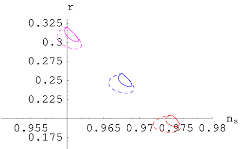
Figure 1: The tensor-to-scalar ratio $r\simeq 16\epsilon_{\lower 2.0pt\hbox{$\scriptstyle H$}}$ vs the scalar spectral index $n_{\lower 2.0pt\hbox{$\scriptstyle s$}}$, with $\alpha=0.21,0.20$ and $0.19$ (top to bottom) and $\zeta=(-0.2,0)$. The solid (dotted) lines are for ${\cal N}_{e}=60$ (${\cal N}_{e}=40$).

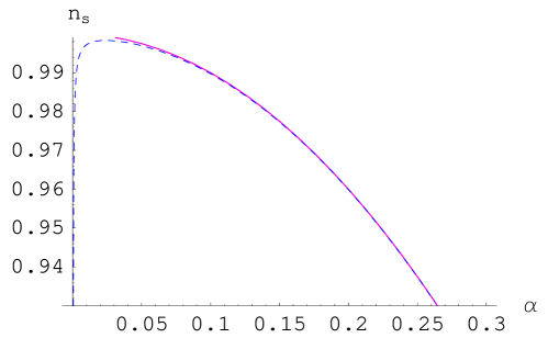
Figure 2: The scalar spectral index $n_{s}$ vs $\alpha$, with ${\cal N}_{e}=70$ (solid line), ${\cal N}_{e}=40$ (dotted line) and $\zeta=\{-2,0\}$. Except for $\alpha<|\zeta|\lesssim 0.05$, the value of $n_{s}$ does not much depend on $\zeta$.

The scalar spectrum on scales accessible to CMB observations is perhaps that measured at the instance when observable scales exit the horizon during inflation. In most models this corresponds to a phase of inflation between e-folds $50$ and $60$. We summarize the results in a Table (for ${\cal N}_{e}=50$ and $\zeta=-0.1$):

	$n_{\lower 2.0pt\hbox{$\scriptstyle s$}}$	$r=16\epsilon_{\lower 2.0pt\hbox{$\scriptstyle H$}}$	$\alpha$	$\eta_{\lower 2.0pt\hbox{$\scriptstyle H$}}$
$r<0.28$	$n_{\lower 2.0pt\hbox{$\scriptstyle s$}}\gtrsim 0.965$	$--$	$<0.18$	$<0.017$
$n_{\lower 2.0pt\hbox{$\scriptstyle s$}}=0.96$	$--$	$0.32$	$0.200$	$0.020$
$r=0.1$	0.987	$--$	$0.112$	$0.006$

In figure 1 we show the plot of tensor-to-scalar ratio $r$ with respect to $n_{s}$, and in figure 2 the plot of $n_{s}$ with respect to $\alpha$. Within our model, both $n_{s}$ and $r$ do not much depend on the number of e-folds except when $\zeta$ is positive, which we reject on physical grounds.

With the WMAP3 bound on the tensor-to-scalar ratio, $r<0.28$, we find $n_{\lower 2.0pt\hbox{$\scriptstyle s$}}\gtrsim 0.965$ for $\zeta\lesssim-0.1$. The bound $r<0.28$ implies that $\varepsilon_{\lower 2.0pt\hbox{$\scriptstyle H$}}<0.0175$ and imposes a relation (for a given $N$) between $\lambda$ and $\alpha$. Using equation (9), we get $n_{s}\gtrsim 0.965$ for $\zeta\leq-0.1$. The scalar spectrum is red-tilted except in the case that $\alpha\lesssim 0$ and both $\zeta$ and $r$ are sufficiently close to zero, e.g., for $\zeta=-0.005$ and $r=0.001$, we get $(\alpha,n_{s},N)=(-0.0051,1.0107,50),(-0.0057,1.0097,60)$.

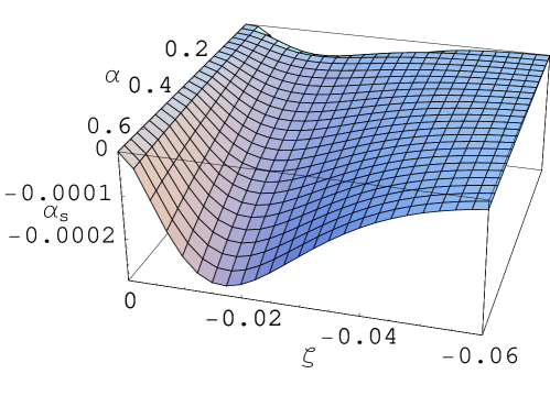
Figure 3: The running of scalar spectral index, $\alpha_{\lower 2.0pt\hbox{$\scriptstyle s$}}$, with respect to $\alpha$ and $\zeta$ with ${\cal N}_{e}=60$. Except for $\alpha<|\zeta|\lesssim 0.05$, $\alpha_{\lower 2.0pt\hbox{$\scriptstyle s$}}$ does not much depend on the number of e-folds.

The running of spectral index, $\alpha_{s}$, is given by

$$\alpha_{s}\equiv\frac{dn_{\lower 2.0pt\hbox{$\scriptstyle s$}}}{d\ln k}=\frac{dn_{s}}{dN}\frac{dN}{d\phi}\frac{d\phi}{d\ln k},$$ (10)

where

$$\frac{d\phi}{d\ln k}=-m_{\lower 2.0pt\hbox{$\scriptstyle P$}}\frac{\sqrt{2\epsilon_{\lower 2.0pt\hbox{$\scriptstyle H$}}(\phi)}}{(1-\epsilon_{\lower 2.0pt\hbox{$\scriptstyle H$}}(\phi))},\quad m_{\lower 2.0pt\hbox{$\scriptstyle P$}}\frac{dN}{d\phi}=-\frac{1}{\sqrt{2\epsilon_{\lower 2.0pt\hbox{$\scriptstyle H$}}(\phi)}}.$$ (11)

These relations hold independent of our ansatz (4). In our model, the value of $\alpha_{s}$ is found to be small, when satisfying $0.01<\alpha<\sqrt{2}$ and $\zeta<0$ (cf figure 3).

We conclude this section with a couple of remarks. Studies in [16] show that, in slow-roll inflation, one may relate the variation of the inflaton in terms of e-folds $N=\ln(a_{f}/a_{i})$ to the tensor-to-scalar ratio $r$

$$\frac{1}{m_{P}}\frac{d\phi}{dN}=\frac{\phi^{\prime}}{m_{P}}=\sqrt{\frac{r}{8}}$$ (12)

The WMAP bound on the tensor-to-scalar ratio is $r<0.28$ ($95\%$ confidence level). This then implies that $\alpha<0.187$ in the present construction. This is completely consistent with our discussion above.

The reconstructed potential may be expressed as

$$V(\varphi)=\frac{H^{2}(\varphi)}{2\kappa^{2}}\left[6-\left(\alpha-2\zeta\varphi-2\alpha\zeta\,N(\varphi)\right)^{2}\right],$$ (13)

where

$$H(\varphi)\propto\exp\left[\frac{\alpha^{2}}{2}N(\varphi)+\alpha{\varphi}-\frac{\zeta}{2}(\varphi+\alpha N(\varphi))^{2}\right],$$ (14)

where $N(\varphi)=\ln[a(\varphi(t))]$ and $\varphi\equiv(\phi-\phi_{\lower 2.0pt\hbox{$\scriptstyle 0$}})/m_{P}$.

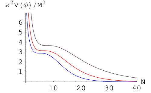
Figure 4: The scalar potential for some representative values of $\alpha=0.3,~{}0.4,~{}0.5$ (top to bottom), $\zeta=-\,0.1$ and $C=-10$.

The shape of the potential (as depicted in figure 4) as well as its functional form is qualitatively similar to a class of scalar potentials one would obtain via warped flux compactifications of string theory, see, e.g. [17]. The predicted characteristics of inflationary phase (of the potential) can easily be made to comply with the WMAP results [1]. So our method of reconstruction may be considered as a point in favour of providing a believable physical basis for the inflation. Moreover, a large part of our construction does not depend on the details of string theory or the dynamics of scalar fields abundant in any higher dimensional theories but has a general validity, and thus would remain useful even if string theory is invalidated.

3 Reheating after inflation

A satisfactory model of inflation should perhaps be followed by a successful reheating. To this end, the ‘instant preheating’ mechanism presented in [18] and applied to exponential potentials in [19] might perhaps be the most efficient method for reheating the universe. Here we briefly outline a viable mechanism of reheating in our model, leaving the details for future publication.

According to (4), after a few e-folds of inflation, since $\zeta N<0$, one has $\dot{\phi}\simeq-\alpha\,m_{\lower 2.0pt\hbox{$\scriptstyle P$}}H$. Clearly, with $\alpha<\sqrt{2}$, the kinetic term never dominates the potential term. As a result there remains the possibility that the expansion enters inflation from which it never recovers. So our model has a chance to work only if the matter and/or radiation energy density terms sometime after inflation is large enough to dominate the inflaton energy density.

Without loss of generality, we can make the inflation end at the origin by translating the field

$$V(\varphi)=M^{2}m_{\lower 2.0pt\hbox{$\scriptstyle P$}}^{2}(3-\alpha^{2}/2)\,\rm e^{\alpha(\varphi/m_{\lower 2.0pt\hbox{$\scriptstyle P$}})}+{\rm small~{}correction},$$ (15)

so after inflation $\varphi\equiv(\phi-\phi_{\rm end})\lesssim 0$. Following [18, 19] we assume that the inflaton field $\varphi$ interacts with another scalar field $\chi$. The interaction Lagrangian is

$${\cal L}_{\rm int}=-\frac{1}{2}g^{2}\varphi^{2}\chi^{2}-h\bar{\psi}\psi\chi,$$ (16)

where $g$ and $h$ are coupling constants, and $\psi$ is a Fermi field. The production of $\chi$ particles commences when the adiabatic condition

$$|\dot{m}_{\chi}|<m_{\chi}^{2}$$ (17)

is violated, i.e. when $|\dot{\varphi}|\gtrsim g\varphi^{2}$, where $m_{\chi}\equiv g|\varphi(t)|$. So, the particle production may occur when

$$|\varphi|\lesssim\sqrt{\frac{\dot{\varphi}_{\rm end}}{g}}\sim\frac{\alpha^{1/2}V^{1/4}_{\rm end}(\varphi)}{3^{1/4}g^{1/2}}\equiv\varphi_{\lower 2.0pt\hbox{$\scriptstyle\rm prod$}}.$$ (18)

The process of particle production occurs nearly instantaneously, within the time

$$\Delta t_{\lower 2.0pt\hbox{$\scriptstyle\rm prod$}}\sim\frac{|\varphi|}{|\dot{\varphi}_{\lower 2.0pt\hbox{$\scriptstyle\rm end$}}|}\sim\frac{V^{-1/4}_{\rm end}(\varphi)}{\alpha^{1/2}g^{1/2}}$$ (19)

during which the field $\varphi$ remains in the vicinity of $\varphi=0$. As the field rolls to $\varphi<0$ direction, the mass of the $\chi$ particles begins to grow, since $m_{\chi}\equiv g|\varphi(t)|$. The occupation number of $\chi$ particles is $n_{k}\sim\rm e^{-\pi(k\Delta t_{\lower 2.0pt\hbox{$\scriptstyle\rm prod$}})^{2}}$, with $k$ being the canonical momemtum. The energy density of particles of the $\chi$ field created in this process is

$$\rho_{\chi}=m_{\chi}n_{\chi}\left(\frac{a_{\lower 2.0pt\hbox{$\scriptstyle\rm end$}}}{a}\right)^{3},$$ (20)

where the number density $n_{\chi}=(2\pi^{3})^{-1}\int_{0}^{\infty}k^{2}n_{k}dk\simeq(2\pi)^{-3}(\alpha g)^{3/2}V_{\lower 2.0pt\hbox{$\scriptstyle\rm end$}}^{3/4}(\varphi)$. If the $\chi$ particles can rapidly decay into fermions or the quanta of the $\chi$ field were to convert (or thermalize) into radiation, then the radiation energy density would increase sharply to

$$\rho_{r}\simeq\rho_{\chi}\sim\frac{g^{5/2}\alpha^{3/2}V^{3/4}_{\lower 2.0pt\hbox{$\scriptstyle\rm end$}}}{8\pi^{3}}\,\varphi_{\lower 2.0pt\hbox{$\scriptstyle\rm prod$}}\sim 0.0027g^{2}\,\alpha^{2}V_{\lower 2.0pt\hbox{$\scriptstyle\rm end$}}(\varphi).$$ (21)

At the end of instant preheating

$$\frac{\rho_{\varphi}}{\rho_{r}}\sim\frac{370}{\alpha^{2}g^{2}}.$$ (22)

Although $\rho_{\chi}/\rho_{\varphi}$ is small quantity to begin with (for any generic value of the coupling $g\lesssim 0.3$ and $\alpha<\sqrt{6}$), $\rho_{\chi}$ (or the decay product of the $\chi$ field) will decrease as $a^{-3(1+w)}$ ($w\leq 1/3$) and come to dominate $\rho_{\lower 2.0pt\hbox{$\scriptstyle\varphi$}}$ since the field $\varphi$ is rolling down an exponential potential and its energy density could decrease much faster $\rho_{\lower 2.0pt\hbox{$\scriptstyle\varphi$}}\propto 1/a^{6}$ after inflation. To illustrate this one considers a cosmic evolution by suppressing $dV/d\varphi$, so $\ddot{\varphi}+3H\dot{\varphi}=0$, whose solution is $\varphi=\varphi_{\lower 2.0pt\hbox{$\scriptstyle 0$}}+\varphi_{\lower 2.0pt\hbox{$\scriptstyle 1$}}\int a^{-3}dt$. According to (4), $\dot{\varphi}\simeq-\alpha\,m_{\lower 2.0pt\hbox{$\scriptstyle P$}}H$ and hence $a(t)=a_{\lower 2.0pt\hbox{$\scriptstyle\rm end$}}\left(t_{\lower 2.0pt\hbox{$\scriptstyle 0$}}+(3/\alpha)t\right)^{1/3}$. We then find

$$\dot{\varphi}^{2}\simeq\frac{\alpha^{2}}{3}\,V(\varphi)\sim 10^{-9}\,m_{\lower 2.0pt\hbox{$\scriptstyle P$}}^{4}\left(\frac{a_{\lower 2.0pt\hbox{$\scriptstyle\rm end$}}}{a}\right)^{6}.$$ (23)

For $\alpha<\sqrt{3}$, there would be no kinetic regime. Nevertheless, since $\rho_{\chi}$ (or the decay products of the $\chi$ field) may decrease much slower $1/[a(t)]^{n}$ ($n\leq 4$) than $\rho_{\phi}$, it will eventually dominate the scalar energy density before the production of light elements or the BBN epoch. Instant preheating may be followed by reheating which occurs through the decay of $\chi$ particles to fermions as is evident from the interaction term in (16).

4 Growing matter

Given that the inflaton field $\phi$ decays to some radiation and heavy particles, it would be natural to expect, at later stages of inflation, small but nonzero values for both the matter and radiation energy densities. The growth in matter energy density can naturally affect (or modify) the form (or shape) of the scalar potential, leading to an additional term in the potential with a relatively large slope. This last feature is perhaps required to make our model compatible with the big-bang nucleosynthesis (BBN) bound imposed on the scalar field energy density.

Here we take the matter Lagrangian in its simplest form, which is Einsteinian

$${\cal L}_{m}\equiv{\cal L}(g_{\mu\nu},\psi_{m})=\sqrt{-g}\left({\rho}_{\lower 2.0pt\hbox{$\scriptstyle M$}}+{\rho}_{\lower 2.0pt\hbox{$\scriptstyle R$}}\right),$$ (24)

where ${\rho}_{\lower 2.0pt\hbox{$\scriptstyle(i)$}}\propto a^{-\,3(1+w_{(i)})}$, $i=M$ (matter) or $R$ (radiation). Of course, one could allow in principle an explicit coupling between the $\phi$-field and matter. It is believed that inflation was followed by an instant preheating (or reheating) and then by a radiation dominated phase, so the strength of coupling between the field $\phi$ and matter could be neglected during both the inflationary and the radiation-dominated epochs. Any such couplings, however, can be relevant at later stages of evolution, especially, at galactic distance scales (see section 6).

The set of autonomous equations of motion that follows from equations (1) and (24) may be given by [20]

$$\kappa^{2}V(\phi) = \left[(3+\epsilon)(1-\Omega_{w})+\frac{1}{2}\,\Omega_{w}^{\,\prime}\right]\,H^{2}(\phi),$$ (25)

$$\kappa^{2}{\phi^{\prime}}^{2} = \Omega_{w}^{\,\prime}-2\epsilon(1-\Omega_{w}),$$ (26)

$$\Omega_{w}^{\,\prime} = -2\epsilon\,\Omega_{w}-3(1+w)\Omega_{w},$$ (27)

where $\Omega_{w}\equiv\Omega_{M}+\Omega_{R}$, the prime denotes a derivative with respect to $N\equiv\ln[a(t)]$, and

$$\phi^{\prime}=\frac{\dot{\phi}}{H},~{}~{}w\equiv\frac{p_{\lower 2.0pt\hbox{$\scriptstyle R$}}+p_{\lower 2.0pt\hbox{$\scriptstyle M$}}}{\rho_{\lower 2.0pt\hbox{$\scriptstyle R$}}+\rho_{\lower 2.0pt\hbox{$\scriptstyle M$}}},~{}~{}\epsilon=\frac{H^{\prime}}{H},~{}~{}\Omega_{i}\equiv\frac{\kappa^{2}\rho_{i}}{3H^{2}}.$$ (28)

During radiation dominance $\Omega_{\lower 2.0pt\hbox{$\scriptstyle\phi$}}$ would remain small but nonzero. This last assumption is consistent with the fact that the fixed point solution $\Omega_{w}=1$ is always unstable. Notice that the behaviour $V(\phi)\propto H^{2}(\phi)$ holds also in the presence of ordinary fields (matter and radiation).

From equations (25)-(27), along with equation (4), we find

$$\kappa^{2}V(\phi) = \frac{H^{2}(\phi)}{\kappa^{2}}\left[3(1-\Omega_{w})-B(\phi)\right],$$ (29)

$$\epsilon(\phi) = -\frac{3}{2}(1+w)\Omega_{w}-B(\phi),$$ (30)

$$\Omega_{w} = \frac{C(\phi)}{C_{\lower 2.0pt\hbox{$\scriptstyle 0$}}+3(1+w)\int(-C(\phi))\,dN(\phi)},$$ (31)

where $C_{\lower 2.0pt\hbox{$\scriptstyle 0$}}$ is an integration constant and

$$B(\phi)\equiv\frac{1}{2}\left(\alpha+2\zeta\rm e^{2\zeta N(\phi)}\right)^{2},$$ (32)

$$C(\phi)=\rm e^{\,\left(\alpha^{2}-3(1+w)\right)N(\phi)}\exp\left[2\alpha\,\rm e^{2\zeta N(\phi)}+\zeta\rm e^{4\zeta N(\phi)}\right].$$ (33)

As compared to the inflationary potential given by equations (13) and (14), we now have the effect of matter fields (matter and radiation together). Of course, in the limit that $\Omega_{\lower 2.0pt\hbox{$\scriptstyle w$}}\to 0$, equation (29) reduces to (13).

During radiation domination, since $\Omega_{\lower 2.0pt\hbox{$\scriptstyle R$}}\gg\Omega_{\lower 2.0pt\hbox{$\scriptstyle M$}}$ and $\Omega_{\lower 2.0pt\hbox{$\scriptstyle w$}}\approx\Omega_{\lower 2.0pt\hbox{$\scriptstyle R$}}$, we have $w\simeq 1/3$. One also notes that the last term in equation (4) does not contribute (significantly) after inflation. Therefore, from equations (29)-(31), we get

$$\Omega_{\lower 2.0pt\hbox{$\scriptstyle w$}}=\frac{1+w-{\alpha}^{2}/3}{1+w}\,\frac{H_{0}^{2}}{H^{2}(\phi)}\,\rm e^{3(1+w)\kappa(\phi-\phi_{2})/\alpha},$$ (34)

where $H^{2}(\phi)=H_{0}^{2}[\rm e^{\alpha\kappa(\phi-\phi_{1})}+\rm e^{3(w+1)\kappa(\phi-\phi_{2})/\alpha}]$, and

$$V(\phi)=\frac{H_{0}^{2}}{\kappa^{2}}\left[\alpha_{\lower 2.0pt\hbox{$\scriptstyle 1$}}\rm e^{3(1+w)\kappa(\phi-\phi_{2})/\alpha}+\alpha_{\lower 2.0pt\hbox{$\scriptstyle 2$}}\rm e^{\alpha\kappa(\phi-\phi_{1})}\right],$$ (35)

where $\alpha_{1}\equiv\frac{\alpha^{2}}{2}\frac{1-w}{1+w}$, $\alpha_{2}\equiv\frac{6-{\alpha}^{2}}{2}$, and $H_{0}$, $\phi_{1}$, $\phi_{2}$ are integration constants; we take $\phi<\phi_{\lower 2.0pt\hbox{$\scriptstyle 2$}}\ll\phi_{\lower 2.0pt\hbox{$\scriptstyle 1$}}$. Exponential potentials of a such form, which also arise ubiquitously in particle physics and string theory models [21], by themselves are a promising ingredient for building a natural model of quintessential inflation. In order for the scalar field potential not to dominate the energy density of the universe during BBN, it is required that $3(1+w)>\sqrt{6}\alpha$, which easily satisfies the bound imposed on $\Omega_{\phi}$ during the nucleosynthesis epoch, $\Omega_{\lower 2.0pt\hbox{$\scriptstyle\phi$}}(1\,{\rm MeV})\lesssim 0.05$ [22]. By taking $\alpha\lesssim 0.8$ and $w\simeq 1/3$, we correctly reproduce a double exponential potential anticipated in [23].

The reason why the quintessential part of the potential, equation (35), has a different form with respect to its inflationary part is easy to understand in our model. During inflation the matter contribution (and its possible coupling with the inflaton field) can be safely neglected. This is, however, essentially not the case for quintessence part. Another source of this difference is that the last term in equation (4) does not contribute (significantly) at later stages of evolution, like during the radiation-dominated epoch.

5 Late time acceleration: Dominance of dark energy

At late times, without loss of generality, one takes ${\rho}_{\lower 2.0pt\hbox{$\scriptstyle R$}}\ll{\rho}_{\lower 2.0pt\hbox{$\scriptstyle M$}}$ and $w\simeq 0$. One also assumes that $\phi$ is rolling only slowly, such that $|\dot{\phi}|/H<m_{\lower 2.0pt\hbox{$\scriptstyle P$}}$. In this case the inflaton potential takes a simpler form, for the evolution of the universe could naturally lead the potential part to dominate the kinetic part: $2V(\phi)\propto\dot{\phi}^{2}$, with $m$ being the proportionality constant. Explicitly, we get

$$V(\phi)=m_{\lower 2.0pt\hbox{$\scriptstyle P$}}^{2}H(\phi)^{2}\,\frac{3m}{m+1}(1-\Omega_{\lower 2.0pt\hbox{$\scriptstyle w$}}),\\$$ (36)

$\epsilon(\phi)=-\frac{3}{m+1}-\frac{3}{2}\,\widetilde{w}\Omega_{\lower 2.0pt\hbox{$\scriptstyle w$}}$ and $\Omega_{\lower 2.0pt\hbox{$\scriptstyle w$}}=1/[1+\delta(z+1)^{-\,3\widetilde{w}}]$, where $z$ is the redshift factor and $\widetilde{w}\equiv w+\frac{m-1}{m+1}$. The Hubble parameter $H(\phi(z))$ (and hence $V(\phi(z))$) can be expressed in a closed form using the relation $\epsilon=\dot{H}/H^{2}$. The numerical constant $\delta$ can also be fixed using observational input: an ideal situation would be that the universe re-enters into an accelerating phase ($\epsilon>-1$) for $z\lesssim 1$. The universe passes from a decelerating phase to an accelerating phase when $\Omega_{\lower 2.0pt\hbox{$\scriptstyle w$}}<\frac{m-2}{2m-1}$. The dark energy equation of state is $w_{\lower 2.0pt\hbox{$\scriptstyle\phi$}}={p_{\lower 2.0pt\hbox{$\scriptstyle\phi$}}}/\rho_{\lower 2.0pt\hbox{$\scriptstyle\phi$}}=\frac{1-2m}{1+2m}$; therefore, with $m\equiv 50$, we get $w_{\rm{eff}}\equiv-1-2\epsilon/3\sim-0.76$ and $w_{\lower 2.0pt\hbox{$\scriptstyle\phi$}}\sim-0.98$ (see also figure 5).

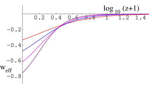
Figure 5: Evolution of the universe passing from matter dominance ($w_{\rm eff}\simeq 0$) to scalar field dominance ($w_{\rm eff}<-1/3$), with $m=3,5,10$ and $50$ (from top to bottom).

The behaviour of dark energy similar to that depicted in figure 5 may be seen directly from equations (34)-(35). Using the relation $e^{N}=e^{\ln a}\equiv(1+z)^{-1}$ and making the assumption that ordinary matter (including cold dark matter) is approximated by a non-relativistic perfect fluid and $\rho_{\lower 2.0pt\hbox{$\scriptstyle R$}}\ll\rho_{\lower 2.0pt\hbox{$\scriptstyle M$}}$, so that $w\approx p_{\lower 2.0pt\hbox{$\scriptstyle M$}}/\rho_{\lower 2.0pt\hbox{$\scriptstyle M$}}\approx 0$, we find

$$\Omega_{\lower 2.0pt\hbox{$\scriptstyle w$}}\simeq\Omega_{\lower 2.0pt\hbox{$\scriptstyle M$}}=\left(1-\frac{\alpha^{2}}{3}\right)\frac{1}{1+c_{\lower 2.0pt\hbox{$\scriptstyle 0$}}\,(1+z)^{\alpha^{2}-3}}$$ (37)

and

$$\epsilon(z)=-1-q(z)=-\frac{3}{2}\Omega_{\lower 2.0pt\hbox{$\scriptstyle M$}}-\frac{\alpha^{2}}{2},$$ (38)

where $q$ is the deceleration parameter. Hence

$$H(z)=H_{\lower 2.0pt\hbox{$\scriptstyle 0$}}\left[\Omega_{\lower 2.0pt\hbox{$\scriptstyle m0$}}(1+z)^{3}+c_{\lower 2.0pt\hbox{$\scriptstyle 0$}}(1-\Omega_{\lower 2.0pt\hbox{$\scriptstyle m0$}})(1+z)^{\alpha^{2}}\right]^{1/2}.$$ (39)

The numerical coefficient $c_{\lower 2.0pt\hbox{$\scriptstyle 0$}}$ may be fixed such that $\Omega_{\lower 2.0pt\hbox{$\scriptstyle M$}}=0.27$ at $z=0$. With $\alpha<\sqrt{2}$, the second term on right-hand side decreases with $z$ at a slower rate as compared to $\rho_{\lower 2.0pt\hbox{$\scriptstyle M$}}$ (which varies as $(1+z)^{3}$) as well as to that of the curvature, $\rho_{\lower 2.0pt\hbox{$\scriptstyle k$}}$ (which varies as $(1+z)^{2}$), so $\Omega_{\lower 2.0pt\hbox{$\scriptstyle\phi$}}$ naturally exhibits ‘dark energy’ as late times. As depicted in figure 6, for $\alpha\simeq 0$, the universe starts to accelerate when $z\lesssim 0.8$. For a larger $\alpha$, acceleration starts at a lower redshift; with a moderate value of $\alpha\simeq 0.26$, we get $w_{\lower 2.0pt\hbox{$\scriptstyle\rm DE$}}=w_{\lower 2.0pt\hbox{$\scriptstyle\phi$}}\simeq(\alpha^{2}-3\Omega_{\lower 2.0pt\hbox{$\scriptstyle\phi$}})/3\Omega_{\lower 2.0pt\hbox{$\scriptstyle\phi$}}\simeq-0.97$.

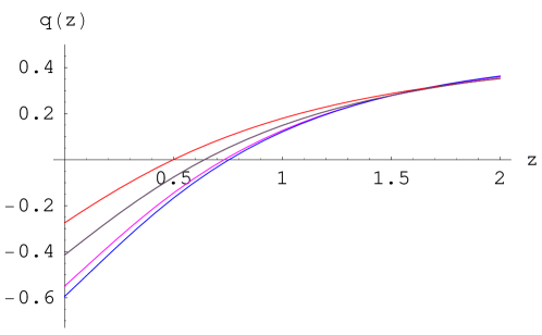
Figure 6: The deceleration parameter $q(z)$ with respect to redshift $z$, and $\alpha=0.8,0.6,0.3,0.01$ (top to bottom). The free parameter $c_{\lower 2.0pt\hbox{$\scriptstyle 0$}}$ in equation (37) is chosen such that $\Omega_{\lower 2.0pt\hbox{$\scriptstyle M0$}}\simeq 0.27$.

The present model addresses the cosmic coincidence problem, only partially. In fact, the cosmic coincidence problem (i.e. why $\rho_{\lower 2.0pt\hbox{$\scriptstyle\phi$}}\simeq 3\rho_{\lower 2.0pt\hbox{$\scriptstyle M$}}$ now?) often involves some kind of fine tuning, and it is not an exception here. An interesting observation is that this last phenomenon requires either a specific ratio between the kinetic and potentials terms, or a specific value for the field velocity $\phi^{\prime}\equiv\kappa\dot{\phi}/H$, which is characterized by the parameter $\alpha$, so as to realize a quintessence dominance for $z\lesssim 0.85$.

6 Evading gravity constraints

In the above discussions we ignored the coupling of the $\phi$-field with matter. This is perhaps justified.

The dark energy or the cosmic acceleration problem is essentially a problem associated with largest cosmological scales: in order for the field $\phi$ to play a role of dark energy its effective mass should be at least in the range of the present value of the Hubble parameter, $H_{\lower 2.0pt\hbox{$\scriptstyle 0$}}\sim 10^{-33}~{}{\rm eV}$. In turn, one takes the runaway quintessence potential satisfying $\sqrt{V(\phi)}\simeq H_{\lower 2.0pt\hbox{$\scriptstyle 0$}}\sim 10^{-33}~{}{\rm eV}$; the range of the interactions mediated by the scalar field $\phi$ can be of the order of the Hubble horizon size. However, Newtonian tests of Einstein’s general relativity and fifth force experiments such as the Cassini satellite experiment put stringent bounds on the gravitational coupling of light scalar particles. That means, a putative dark energy field should be sufficiently massive at much smaller scales. Thus a mechanism similar to that in Chameleon field theory [24], which combines both a quintessence-like behaviour leading to dark energy at late time and a gravitational coupling to matter which is appreciable in high density regions, could be operative in our model.

To this reason, one allows a nontrivial coupling between the $\phi$-field and matter, and, accordingly, takes the matter Lagrangian in a general form

$${\cal L}_{m}={\cal L}(\psi_{\lower 2.0pt\hbox{$\scriptstyle m$}},A^{2}(\phi)g_{\mu\nu})\equiv\sqrt{-g}\,A^{4}(\phi)\sum\widetilde{\rho}_{\lower 2.0pt\hbox{$\scriptstyle(i)$}},$$ (40)

where $\widetilde{\rho}_{\lower 2.0pt\hbox{$\scriptstyle(i)$}}\propto{\hat{a}}^{-3\left(1+w_{i}\right)}$, $\hat{a}\equiv aA(\phi)$. $\phi$ couples to the trace of the matter stress tensor, $g_{(i)}^{\mu\mu}T_{\mu\nu}^{(i)}$, so the radiation term $\widetilde{\rho}_{\lower 2.0pt\hbox{$\scriptstyle R$}}$ does not contribute to the equation of motion for $\phi$

$$\dot{\rho}_{\lower 2.0pt\hbox{$\scriptstyle\phi$}}+3H\rho_{\lower 2.0pt\hbox{$\scriptstyle\phi$}}\left(1+w_{\lower 2.0pt\hbox{$\scriptstyle\phi$}}\right)=-\dot{\phi}\eta\alpha_{\lower 2.0pt\hbox{$\scriptstyle\phi$}}A(\phi)\rho_{\lower 2.0pt\hbox{$\scriptstyle M$}},$$ (41)

where $\eta\equiv(1-3w_{i})$, $\rho_{\lower 2.0pt\hbox{$\scriptstyle\phi$}}\equiv\frac{1}{2}\dot{\phi}^{2}+V(\phi)$, $w_{\lower 2.0pt\hbox{$\scriptstyle\phi$}}\equiv p_{\lower 2.0pt\hbox{$\scriptstyle\phi$}}/\rho_{\lower 2.0pt\hbox{$\scriptstyle\phi$}}$, $w_{\lower 2.0pt\hbox{$\scriptstyle i$}}\equiv p_{\lower 2.0pt\hbox{$\scriptstyle i$}}/\rho_{\lower 2.0pt\hbox{$\scriptstyle i$}}$ and $\alpha_{\lower 2.0pt\hbox{$\scriptstyle\phi$}}\equiv\frac{d\ln A(\phi)}{d(\kappa\,\phi)}$. Equation (41), along with the equation of motion for ordinary fluids

$$\dot{\rho}_{i}+3H\rho_{i}(1+w_{i})=+\dot{\phi}\eta\alpha_{\lower 2.0pt\hbox{$\scriptstyle\phi$}}A(\phi)\rho_{i},\quad(i=M,R),$$ (42)

guarantees the conservation of total energy, namely $\dot{\rho}+3H(\rho+p)=0$, where $\rho\equiv\rho_{\lower 2.0pt\hbox{$\scriptstyle M$}}+\rho_{\lower 2.0pt\hbox{$\scriptstyle R$}}+\rho_{\lower 2.0pt\hbox{$\scriptstyle\phi$}}$.

In the discussion below we take $w_{\lower 2.0pt\hbox{$\scriptstyle M$}}=0$. The effective scalar potential is then given by

$$V_{\lower 2.0pt\hbox{$\scriptstyle\rm eff$}}\equiv V(\phi)+{\rho}_{\lower 2.0pt\hbox{$\scriptstyle M$}}\int\alpha_{\lower 2.0pt\hbox{$\scriptstyle\phi$}}A(\phi)\,d\phi,$$ (43)

where ${\rho}_{\lower 2.0pt\hbox{$\scriptstyle M$}}\propto 1/a^{3}$. For $|\alpha_{\lower 2.0pt\hbox{$\scriptstyle\phi$}}|>0$, the model needs to be confronted with the present-day equivalence principle bound, $\alpha_{\lower 2.0pt\hbox{$\scriptstyle\phi$}}^{2}\leq 5\times 10^{-5}$. On largest scales probed by WMAP, where ${\rho}_{\lower 2.0pt\hbox{$\scriptstyle M$}}\simeq\rho_{\lower 2.0pt\hbox{$\scriptstyle\rm crit$}}\simeq{10}^{-12}~{}({\rm eV})^{4}$ (where $\rho_{\lower 2.0pt\hbox{$\scriptstyle\rm crit$}}\equiv 3H_{\lower 2.0pt\hbox{$\scriptstyle 0$}}^{2}/8\pi G_{\lower 2.0pt\hbox{$\scriptstyle N$}}$ is the critical energy density), the last term above is only sub-leading, which is suppressed by a factor of $\alpha_{\lower 2.0pt\hbox{$\scriptstyle\phi$}}$. In turn, $\phi$ can be sufficiently light, $m_{\lower 2.0pt\hbox{$\scriptstyle\phi$}}\equiv V_{\lower 2.0pt\hbox{$\scriptstyle\phi\phi$}}^{1/2}\sim 10^{-33}\,{\rm eV}\sim(10^{28}{\rm cm})^{-1}$, and its energy density may evolve slowly over cosmological time-scales. But within solar system distances, where ${\rho}_{\lower 2.0pt\hbox{$\scriptstyle M$}}$ is roughly $10^{23}$ times larger than its value on large (Hubble) scales, the term proportional to ${\rho}_{\lower 2.0pt\hbox{$\scriptstyle M$}}$ can be more relevant. On Earth, ${\rho}_{\lower 2.0pt\hbox{$\scriptstyle M$}}\sim 10^{30}\times\rho_{\lower 2.0pt\hbox{$\scriptstyle\rm crit$}}$, the Compton wavelength of the field $\phi$ can be sufficiently small, $\lambda_{c}\sim m_{\varphi}^{-1}\sim 0.1~{}{\rm mm}$ as to satisfy local tests of gravity. That is, in high density (and high curvature) regions the quintessence field $\phi$ may end up almost in a squeezed state.

7 Further generalization

Although the model above is canonical in describing the basic ideas of quintessence, there exist theoretical and phenomenological motivations for studying modifications of the Einstein-Hilbert action which allow non-trivial couplings of $\phi$ to some quadratic Reimann invariants (of the Gauss-Bonnet form ${\cal R}^{2}\equiv R_{\mu\nu\lambda\sigma}R^{\mu\nu\lambda\sigma}-4{R_{\mu}\nu}R^{\mu\nu}+R^{2}$) and antisymmetric tensor fields [25, 26]

$${\cal L}=\sqrt{-g}\left(\frac{R}{2\kappa^{2}}+{\cal L}(\phi)-{\cal F}(\phi){\cal R}^{2}-{\cal G}(\phi){\cal H}^{2}\right)+{\cal L}_{m},$$ (44)

where ${\cal L}(\phi)=-\frac{1}{2}(\partial\phi)^{2}-V(\phi)$, ${\cal H}^{2}={\cal H}_{\lower 2.0pt\hbox{$\scriptstyle\mu\nu\lambda$}}{\cal H}^{\mu\nu\lambda}$ and ${\cal H}_{\lower 2.0pt\hbox{$\scriptstyle\mu\nu\lambda$}}=\partial_{[\mu}B_{\nu\lambda]}$ is the antisymmetric 3-form field strength. Allowing ${\cal G}(\phi)\neq 0$ in (44), one introduces a pseudoscalar degree of freedom $\sigma$, via the ansatz ${\cal H}_{\mu\nu\lambda}\equiv\sqrt{g}\,\epsilon_{\mu\nu\lambda\tau}\partial^{\tau}\sigma$. Like $\phi$, the axion field $\sigma$ is a function only of time. In particular, the coupling ${\cal F}(\phi)$ allows new cosmological solutions for which the dark energy equation of state can be less than $-1$. To be precise, we note that

$$\frac{\kappa^{2}(\rho_{\lower 2.0pt\hbox{$\scriptstyle DE$}}+p_{\lower 2.0pt\hbox{$\scriptstyle DE$}})}{H^{2}}=\kappa^{2}{\phi^{\prime}}^{2}+(1-\epsilon)\Omega_{\lower 2.0pt\hbox{$\scriptstyle\cal F$}}+\Omega_{\lower 2.0pt\hbox{$\scriptstyle\cal F$}}^{\prime},$$ (45)

where $\Omega_{\lower 2.0pt\hbox{$\scriptstyle\cal F$}}=8\dot{\cal F}H=8{\cal F}^{\prime}H^{2}$. The antisymmetric 3-form field does not modify this equation because it contributes to $\rho_{\lower 2.0pt\hbox{$\scriptstyle DE$}}$ and $p_{\lower 2.0pt\hbox{$\scriptstyle DE$}}$ with the same magnitude but with opposite signs, namely, $\kappa^{2}\rho_{\lower 2.0pt\hbox{$\scriptstyle DE$}}/H^{2}=x^{2}/2+y^{2}+3\Omega_{\lower 2.0pt\hbox{$\scriptstyle\cal F$}}+3\Omega_{\lower 2.0pt\hbox{$\scriptstyle\cal G$}}$ and $\kappa^{2}p_{\lower 2.0pt\hbox{$\scriptstyle DE$}}/H^{2}=x^{2}/2-y^{2}-(2+\epsilon)\Omega_{\lower 2.0pt\hbox{$\scriptstyle\cal F$}}-\Omega_{\lower 2.0pt\hbox{$\scriptstyle\cal F$}}^{\prime}-3\Omega_{\lower 2.0pt\hbox{$\scriptstyle\cal G$}}$, where $\Omega_{\lower 2.0pt\hbox{$\scriptstyle\cal G$}}\equiv 2{\cal G}(\phi)\,\sigma^{\prime\,2}$, $x\equiv\kappa\dot{\phi}/H$ and $y\equiv\kappa\sqrt{V}/H$. We can get $w_{\lower 2.0pt\hbox{$\scriptstyle\phi$}}\equiv\rho_{\lower 2.0pt\hbox{$\scriptstyle\phi$}}/p_{\lower 2.0pt\hbox{$\scriptstyle\phi$}}<-1$, without requiring a superluminal expansion $\epsilon=\dot{H}/H^{2}>0$, or having to introduce a non-canonical (phantom) field. Most features of the model (1) would arise in the limit where ${\cal F}(\phi){\cal R}^{2}$ and ${\cal G}(\phi){\cal H}^{2}$ are sub-leadings to $V(\phi)$ (see below).

In the above model, the axion field $\sigma$ does not play much role. With a generic choice of ${\cal G}(\Phi)\equiv{\cal G}_{\lower 2.0pt\hbox{$\scriptstyle 0$}}e^{2\Phi}$ (where $\Phi\equiv\phi/m_{\lower 2.0pt\hbox{$\scriptstyle P$}}$), the $B$-field equation of motion, $\nabla_{\mu}\left(e^{2\Phi}H^{\mu\nu\lambda}\right)=0$, is solved for $H^{\mu\nu\lambda}=e^{-2\Phi}\epsilon^{\mu\nu\lambda\tau}\partial_{\tau}\sigma$. The integrability condition, $\partial_{[\mu}H_{\nu\lambda\tau]}=0$, yields $\ddot{\sigma}+3H\dot{\sigma}+2\dot{\Phi}\dot{\sigma}=0$. With the ansatz (4), we get

$$\frac{m_{\lower 2.0pt\hbox{$\scriptstyle P$}}\dot{\sigma}}{H^{2}}\propto\exp\left[(2\alpha-3)N+2\zeta e^{2\zeta N}\right].$$ (46)

After a few e-folds of inflation, the last term above would become small, since $\zeta N<0$. The scalar potential reads

$$V(\phi)=\frac{H^{2}}{2}\left[6-\alpha^{2}-12{\cal G}_{\lower 2.0pt\hbox{$\scriptstyle 0$}}e^{2(3/\alpha-1)\Phi}\right],$$ (47)

where $H=H_{\lower 2.0pt\hbox{$\scriptstyle 0$}}\exp[{\alpha\Phi/2}]$. This result in conjunction with equations (4) and (46) implies that for $\alpha<2$, ${\cal G}(\phi){\cal H}^{2}$ decreases faster than the scalar potential $V(\phi)$.

Next we briefly discuss some qualitative features of the reconstructed scalar potential with a nonzero ${\cal F}(\phi)$. With the ansatz (4), and with ${\cal G}(\phi)=0$, the reconstructed potential is given by equation (5); the parameter $\varepsilon_{\lower 2.0pt\hbox{$\scriptstyle H$}}(\phi)$ reads

$$\varepsilon_{\lower 2.0pt\hbox{$\scriptstyle H$}}(\phi) = \frac{1}{2}(\alpha+2\zeta X)^{2}+3\Omega_{\lower 2.0pt\hbox{$\scriptstyle\cal F$}}$$ (48)

$$= \frac{1}{2}(\alpha+2\zeta X)^{2}-24H^{2}(\alpha+2\zeta X)\frac{d{\cal F}(\phi)}{d\phi}.$$

Clearly, in the case $\Omega_{\lower 2.0pt\hbox{$\scriptstyle\cal F$}}<0$, the coupling ${\cal F}(\phi)$ could increase the period of inflation by making $\epsilon_{\lower 2.0pt\hbox{$\scriptstyle H$}}$ smaller. This effect can be opposite in the case $\Omega_{\lower 2.0pt\hbox{$\scriptstyle\cal F$}}>0$: it could be that inflation ended due to a slowly increasing derivative of the coupling, $d{\cal F}/d\phi$, such that $\Omega_{\lower 2.0pt\hbox{$\scriptstyle\cal F$}}\sim 1/3$.

With ${\cal F}(\phi)\neq 0$, the corresponding potential may be reconstructed by providing an extra condition or by demanding a specific relation between the functions $V(\phi)$ and ${\cal F}(\phi)$ (see, e.g. [27], where a general method of reconstruction was developed, including the effect of scalar-Gauss-Bonnet coupling). In the particular case that $a(t)\simeq a_{\lower 2.0pt\hbox{$\scriptstyle 0$}}e^{H_{\lower 2.0pt\hbox{$\scriptstyle 0$}}t}$, we find

$$\Omega_{\lower 2.0pt\hbox{$\scriptstyle\cal F$}}=-\frac{e^{N(\phi)}}{3H_{\lower 2.0pt\hbox{$\scriptstyle 0$}}^{2}}-\alpha^{2}-\frac{4\alpha\zeta}{1-2\zeta}\,e^{2\zeta N(\phi)}-\frac{4\zeta^{2}}{1-4\zeta}\,e^{4\zeta N(\phi)},$$ (49)

where $N(\phi)\equiv\ln a(\phi(t))$+ const. Again, after a few e-folds of inflation, since $\exp[2\zeta N(\phi)]\ll 1$, we get

$$\Omega_{\lower 2.0pt\hbox{$\scriptstyle\cal F$}}=-\alpha^{2}-\frac{e^{N(\phi)}}{3H_{\lower 2.0pt\hbox{$\scriptstyle 0$}}^{2}},\quad\frac{V(\phi)}{3H^{2}}=1+\frac{5}{2}\alpha^{2}+\frac{e^{N(\phi)}}{3H_{\lower 2.0pt\hbox{$\scriptstyle 0$}}^{2}}.$$ (50)

This result reveals a generic situation that the coupled Gauss-Bonnet term is only subleading to the potential $V(\phi)$. This behavior of our model may be present also when the Hubble parameter changes appreciably with e-folding time, as happens at later stages of inflation.

The presence of ordinary fields (matter and radiation) in our model does not introduce much complication, apart from slightly modified expressions for $V(\phi)$ and ${\cal F}(\phi)$, for the added degrees of freedom come with additional equations of motion.

8 Conclusion

We have presented an explicit cosmological model for evolution from inflation to the present epoch that we believe satisfies the main observational constraints, including fine details of the power spectrum of cosmic microwave background anisotropies, e.g., a red-tilted scalar spectrum with small tensor-to-scalar ratio, $r<0.28$, the bound imposed on $\Omega_{\lower 2.0pt\hbox{$\scriptstyle\phi$}}$ during the nucleosynthesis epoch and present epoch local gravity tests. It is therefore potentially of great utility.

In our analysis, just one assumption, equation (4), that is regarding the evolution of inflaton field, has been made, which is indeed a common feature of many motivated slow-roll type inflationary models. Moreover, for a slowly rolling inflaton field, $m_{\lower 2.0pt\hbox{$\scriptstyle P$}}\phi^{\prime}=m_{\lower 2.0pt\hbox{$\scriptstyle P$}}\frac{d\phi}{dN}<0.25$, the gravity waves or the amplitude of tensor perturbations can be suppressed in our model. This might actually be needed in our model, in order to satisfy the BBN bound.

The present proposal also simplifies the role of the inflaton by almost decoupling it from the (background) matter on large cosmological scales. On the scale of the solar system, due to the large surrounding matter density, the dark energy field can be sufficiently massive, e.g., $m_{\lower 2.0pt\hbox{$\scriptstyle\phi$}}\sim\sqrt{\Lambda_{{\rm eff},\,\phi\phi}}\gtrsim 10^{-3}~{}{\rm eV}$, thereby quenching the deviations from Einstein’s gravity on distances larger than a fraction of millimeter. Moreover, the model possesses an attractor behaviour for the inflaton and matter densities analogous to the tracking solution of, e.g., the inverse power-law potential, $V(\phi)\propto\phi^{-\alpha}$ with $\alpha\geq 2$.

The model proposed here may provide a reasonable explanation to the question: why is the cosmological vacuum energy small? The interpretation of gravitational vacuum energy (or dark energy) in our framework is likely to yield $V(\phi)\leq 3(1-\Omega_{\lower 2.0pt\hbox{$\scriptstyle m0$}})H_{\lower 2.0pt\hbox{$\scriptstyle 0$}}^{2}m_{\lower 2.0pt\hbox{$\scriptstyle P$}}^{2}$ and exhibit scaling behaviour for $\rho_{\phi}$, being proportional to the square of the Hubble rate. As a result, within our model, $\rho_{\lower 2.0pt\hbox{$\scriptstyle\phi$}}\simeq 2H_{\lower 2.0pt\hbox{$\scriptstyle 0$}}^{2}m_{\lower 2.0pt\hbox{$\scriptstyle P$}}^{2}=2\times 10^{-66}~{}{\rm eV}^{2}m_{\lower 2.0pt\hbox{$\scriptstyle P$}}^{2}\simeq 3.5\times 10^{-47}({\rm GeV})^{4}$ would be the most probable value of dark energy density at the present epoch.

Acknowledgments

The author acknowledges the hospitality of the Theory Group at CERN and DAMTP (University of Cambridge), where part of this work was carried out. This research is supported in part by the FRST Research Grant E5229 (New Zealand) and Elizabeth Ellen Dalton research Award (2007).

Note added: In our model, for $47<N<70$, there also exists a small window in the parameter space, namely $\alpha=0.011\pm 0.002$ and $\zeta=-0.03\pm 0.02$, for which $n_{s}=0.96\pm 0.01$ and $r\sim{\cal O}(10^{-3}-10^{-4}$), see also [28] for other details. This result is compatible with WMAP5 data [29].

References

References

• [1] D. N. Spergel et al. [WMAP Collaboration] Astrophys. J. Suppl.  148, 175 (2003) D. N. Spergel et al. [WMAP3 Collaboration], Astrophys. J. Suppl. 170, 377 (2007)
• [2] For a review, see e.g., A. Linde, Particle Physics and Inflationary Cosmology, (1990) (New Jersey: Harwood)
• [3] A. G. Riess et al. [Supernova Search Team Collaboration], Astron. J.  116, 1009 (1998) [astro-ph/9805201] S. Perlmutter et al. [Supernova Cosmology Project Collaboration] Astrophys. J. 517, 565 (1999)
A. G. Riess et al. [Supernova Search Team Collaboration] Astrophys. J. 607, 665 (2004)
• [4] B. Boisseau, G. Esposito-Farese, D. Polarski and A. A. Starobinsky, Phys. Rev. Lett.  85, 2236 (2000) [gr-qc/0001066]
• [5] S. Nojiri and S. D. Odintsov, Gen. Rel. Grav.  38, 1285 (2006) [hep-th/0506212] S. Capozziello, S. Nojiri and S. D. Odintsov, Phys. Lett.  B 632, 597 (2006)
• [6] E. J. Copeland, M. Sami and S. Tsujikawa, Int. J. Mod. Phys.  D 15, 1753 (2006)
• [7] P. J. E. Peebles and A. Vilenkin, Phys. Rev.  D 59, 063505 (1999)
• [8] P. J. E. Peebles and B. Ratra, Astrophys. J. 325, L17 (1988) C. Wetterich, Nucl. Phys.  B 302, 668 (1988)
• [9] I. Zlatev, L. M. Wang and P. J. Steinhardt, Phys. Rev. Lett.  82, 896 (1999)
• [10] V. Sahni, M. Sami and T. Souradeep, Phys. Rev.  D 65, 023518 (2002) [gr-qc/0105121] M. Sami and N. Dadhich, TSPU Vestnik 44N7, 25 (2004) [hep-th/0405016]
• [11] M. Giovannini, Class. Quant. Grav.  16, 2905 (1999) [hep-ph/9903263] M. Peloso and F. Rosati, JHEP 9912, 026 (1999) [hep-ph/9908271]
• [12] I. Antoniadis, J. Rizos and K. Tamvakis, Nucl. Phys.  B 415, 497 (1994) [hep-th/9305025] I. P. Neupane, arXiv:hep-th/0605265
• [13] A. Linde, arXiv:0705.0164 [hep-th]
• [14] F. Vernizzi and D. Wands, JCAP 0605, 019 (2006) [astro-ph/0603799]
• [15] E. D. Stewart and D. H. Lyth, Phys. Lett.  B 302, 171 (1993) [gr-qc/9302019]
• [16] D. H. Lyth, Phys. Rev. Lett.  78, 1861 (1997) [hep-ph/9606387] (see also, D. Baumann and L. McAllister, Phys. Rev.  D 75, 123508 (2007) [hep-th/0610285])
• [17] D. Baumann, A. Dymarsky, I. R. Klebanov and L. McAllister, arXiv:0706.0360 S. Panda, M. Sami and S. Tsujikawa, Phys. Rev.  D 76, 103512 (2007) [arXiv:0707.2848]
• [18] G. N. Felder, L. Kofman and A. D. Linde, Phys. Rev. D 59, 123523 (1999) G. N. Felder, L. Kofman and A. D. Linde, Phys. Rev. D 60, 103505 (1999)
• [19] M. Sami and V. Sahni, Phys. Rev.  D 70, 083513 (2004) H. Tashiro, T. Chiba and M. Sasaki, Class. Quant. Grav.  21, 1761 (2004)
• [20] I. P. Neupane, Class. Quant. Grav.  23, 7493 (2006) [hep-th/0602097] B. M. Leith and I. P. Neupane, JCAP 0705 (2007) 019 [hep-th/0702002]
• [21] I. P. Neupane, Class. Quant. Grav.  21, 4383 (2004) [hep-th/0311071] I. P. Neupane and D. L. Wiltshire, Phys. Lett.  B 619, 201 (2005) [hep-th/0502003] I. P. Neupane, Phys. Rev. Lett.  98, 061301 (2007) [hep-th/0609086]
• [22] P. G. Ferreira and M. Joyce, Phys. Rev. Lett.  79, 4740 (1997) E. J. Copeland, A. R. Liddle and D. Wands, Phys. Rev. D 57, 4686 (1998) R. Bean, S. H. Hansen and A. Melchiorri, Phys. Rev.  D 64, 103508 (2001)
• [23] T. Barreiro, E. J. Copeland and N. J. Nunes, Phys. Rev.  D 61, 127301 (2000)
• [24] T. Damour and K. Nordtvedt, Phys. Rev. Lett.  70, 2217 (1993) (see also J. Khoury and A. Weltman, Phys. Rev. Lett.  93, 171104 (2004); D. F. Mota and D. J. Shaw, Phys. Rev.  D 75, 063501 (2007))
• [25] E. S. Fradkin and A. A. Tseytlin, Nucl. Phys.  B 261, 1 (1985) N. Mavromatos and J. Miramontes, Phys. Lett. B 201, 473 (1988) E. J. Copeland, A. Lahiri and D. Wands, Phys. Rev.  D 50, 4868 (1994)
• [26] S. Nojiri, S. D. Odintsov and M. Sasaki, Phys. Rev.  D 71, 123509 (2005) I. P. Neupane and B. M. N. Carter, Phys. Lett. B 638, 94 (2006) [hep-th/0510109] I. P. Neupane and B. M. N. Carter, JCAP 0606, 004 (2006) [hep-th/0512262]
• [27] S. Nojiri and S. D. Odintsov, J. Phys. Conf. Ser. 66, 012005 (2007) G. Cognola, E. Elizalde, S. Nojiri, S. Odintsov and S. Zerbini, Phys. Rev.  D 75, 086002 (2007).
• [28] I. P. Neupane and C. Scherer, JCAP 0805, 009 (2008) [arXiv:0712.2468]
• [29] E. Komatsu et al. [WMAP5 Collaboration], arXiv:0803.0547 [astro-ph]