Analysis of Inter-Domain Traffic Correlations: Random Matrix Theory Approach

Abstract

The traffic behavior of University of Louisville network with the interconnected backbone routers and the number of Virtual Local Area Network (VLAN) subnets is investigated using the Random Matrix Theory (RMT) approach. We employ the system of equal interval time series of traffic counts at all router to router and router to subnet connections as a representation of the inter-VLAN traffic. The cross-correlation matrix $C$ of the traffic rate changes between different traffic time series is calculated and tested against null-hypothesis of random interactions.

The majority of the eigenvalues $\lambda_{i}$ of matrix $C$ fall within the bounds predicted by the RMT for the eigenvalues of random correlation matrices. The distribution of eigenvalues and eigenvectors outside of the RMT bounds displays prominent and systematic deviations from the RMT predictions. Moreover, these deviations are stable in time.

The method we use provides a unique possibility to accomplish three concurrent tasks of traffic analysis. The method verifies the uncongested state of the network, by establishing the profile of random interactions. It recognizes the system-specific large-scale interactions, by establishing the profile of stable in time non-random interactions. Finally, by looking into the eigenstatistics we are able to detect and allocate anomalies of network traffic interactions.

Department of Computer Engineering and Computer Science, University of Louisville, Louisville, KY 40292 email: {vbrozh01, mmkant01}@gwise.louisville.edu

Categories and Subject Descriptors

C.2.3 [Computer-Communication Networks]: Network Operations

General Terms

Measurement, Experimentation

I introduction

The infrastructure, applications and protocols of the system of communicating computers and networks are constantly evolving. The traffic, which is an essence of the communication, presently is a voluminous data generated on minute-by-minute basis within multi-layered structure by different applications and according to different protocols. As a consequence, there are two general approaches in analysis of the traffic and in modeling of its healthy behavior. In the first approach, the traffic analysis considers the protocols, applications, traffic matrix and routing matrix estimates, independence of ingress and egress points and much more. The second approach treats the infrastructure between the points from which the traffic is obtained as a “black box” [33, 34].

Measuring interactions between logically and architecturally equivalent substructures of the system is a natural extension of the “black box” approach. Certain amount of work in this direction has already been done. Studies on statistical traffic flow properties revealed the “congested”, “fluid” and “transitional” regimes of the flow at a large scale [1, 2]. The observed collective behavior suggests the existence of the large-scale network-wide correlations between the network subparts. Indeed, the [3] work showed the large-scale cross-correlations between different connections of the Renater scientific network. Moreover, the analysis of correlations across all simultaneous network-wide traffic has been used in network distributed attacks detection [4].

The distributions and stability of established interactions statistics represent the characteristic features of the system and may be exploited in healthy network traffic profile creation, which is an essential part of network anomaly detection. As it is successfully demonstrated in [5], all tested traffic anomalies change the distribution of the traffic features.

Among numerous types of traffic monitoring variables, time series of traffic counts are free of applications “semantics” and thus more preferable for “black box” analysis. To extract the meaningful information about underlying interactions contained in time series, the empirical correlation matrix is a usual tool at hand. In addition, there are various classes of statistical tools, such as principal component analysis, singular value decomposition, and factor analysis, which in turn strongly rely on the validity of the correlation matrix and obtain the meaningful part of the time series. Thus, it is important to understand quantitatively the effect of noise, i.e. to separate the noisy, random interactions from meaningful ones. In addition, it is crucial to consider the finiteness of the time series in the determination of the empirical correlation, since the finite length of time series available to estimate cross correlations introduces “measurement noise” [19]. Statistically, it is also advisable to develop null-hypothesis tests in order to check the degree of statistical validity of the results obtained against cases of purely random interactions.

The methodology of random matrix theory (RMT) developed for studying the complex energy levels of heavy nuclei and is given a detailed account in [6, 7, 8, 9, 10, 11]. For our purposes this methodology comes in as a series of statistical tests run on the eigenvalues and eigenvectors of “system matrix”, which in our case is traffic time series cross-correlation matrix $C$ (and is Hamiltonian matrix in case of nuclei and other RMT systems [6, 7, 8, 9, 10, 11]).

In our study, we propose to investigate the network traffic as a complex system with a certain degree of mutual interactions of its constituents, i.e. single-link traffic time series, using the RMT approach. We concentrate on the large scale correlations between the time series generated by Simple Network Manage Protocol (SNMP) traffic counters at every router-router and router-VLAN subnet connection of University of Louisville backbone routers system.

The contributions of this study are as follows:

• We propose the application constraints free methodology of network-wide traffic time series interactions analysis. Even though in this particular study, we know in advance that VLANs represent separate broadcast domains, VLAN-router incoming traffic is a traffic intended for other VLANs and VLAN-router outgoing traffic is a routed traffic from other VLANs. Nevertheless, this information is irrelevant for our analysis and acquired only at the interpretation of the analysis results.

• Using the RMT, we are able to separate the random interactions from system specific interactions. The vast majority of traffic time series interact in random fashion. The time stable random interactions signify the healthy, and free of congestion traffic. The proposed analysis of eigenvector distribution allows to verify the time series content of uncongested traffic.

• The time stable non-random interactions provide us with information about large-scale system-specific interactions.

• Finally, the temporal changes in random and non-random interactions can be detected and allocated with eigenvalues and eigenvectors statistics of interactions.

The organization of this paper is as follows. Section II presents the survey of related work. We describe the RMT methodology in Section III. Section IV contains the explanation of the data analyzed. In Section V we test the eigenvalue distribution of inter-VLAN traffic time series cross-correlation matrix C against the RMT predictions. In Section VI we analyze the content of inter-VLAN traffic interactions by mean of eigenvalues and eigenvectors deviated from RMT. Section VII discusses the characteristic traffic interactions parameters of the system such as time stability of the deviating eigenvalues and eigenvectors, inverse participation ratio (IPR) of eigenvalues spectra, localization points in IPR plot, overlap matrices of the deviating eigenvectors. With series of different experiments, we demonstrate how traffic interactions anomalies can be detected and allocated in time and space using various visualization techniques on eigenvalues and eigenvectors statistics in Section VIII. We present our conclusions and prospective research steps in Section IX.

II related work

Few works investigate the interactions of traffic time series regardless of underlying architecture of the traffic system. As it was stated in Introduction, the study of [3] showed the large-scale cross-correlations between different connections of the French scientific network Renater with 26 interconnected routers and 650 connections links. The random interactions between traffic time series of complex traffic system without the routing protocol information were established by Krbalek and Seba in [12] for transportation system in Cuernavaca (Mexico).

The urgent need for a network-wide, scalable approach to the problem of healthy network traffic profile creation is expressed in works of [5, 14, 15, 13, 16, 17]. There are several studies with the promising results, which demonstrate that the traffic anomalous events cause the temporal changes in statistical properties of traffic features. Lakhina, Crovella and Diot presented the characterization of the network-wide anomalies of the traffic flows. The authors studied three different types of traffic flows and fused the information from flow measurements taken throughout the entire network. They obtained and classified a different set of anomalies for different traffic types using the subspace method [14].

The same group of researchers extended their work in [5]. Under the new assumption that any network anomaly induces the changes in distributional aspects of packet header fields, they detected and identified large set of anomalies using the entropy measurement tool.

Hidden Markov model has been proposed to model the distribution of network-wide traffic in [15]. The observation window is used to distinguish denial of service (DoS) flooding attack mixed with the normal background traffic.

Roughan et al. combined the entire network routing and traffic data to detect the IP forwarding anomalies [16].

Huang et al., [17] used the distributed version of the Principal Component Analysis (PCA) method for centralized network-wide volume anomaly detection. A key ingredient of their framework is an analytical method based on stochastic matrix perturbation theory that balances between the accuracy of the approximate network anomaly detection and the amount of data communication over the network.

The authors of [13] found the high temporal correlation (frequently > 0.99) between flow counts on quiescent ports (TCP/IP ports which are not in regular use) at the one of the known pre-attack, so called reconnaissance, anomalous behavior, vertical scan.

III rmt methodology

The RMT was employed in the financial studies of stock correlations [18, 19], communication theory of wireless systems [20], array signal processing [21], bioinformatics studies of protein folding [22]. We are not aware of any work, except for [3], where RMT techniques were applied to the Internet traffic system.

We adopt the methodology used in works on financial time series correlations (see [18, 19] and references therein) and later in [3], which discusses cross-correlations in Internet traffic. In particular, we quantify correlations between $N$ traffic counts time series of $L$ time points, by calculating the traffic rate change of every time series $T$ $i=1,\dots,N$ , over a time scale $\Delta t$,

$$G_{i}\left(t\right)\equiv\textrm{ln}\,T_{i}\left(t+\Delta t\right)-\textrm{ln}\,T_{i}\left(t\right)$$ (1)

where $T{}_{i}\left(t\right)$ denotes the traffic rate of time series $i$. This measure is independent from the volume of the traffic exchange and allows capturing the subtle changes in the traffic rate [3]. The normalized traffic rate change is

$$g_{i}\left(t\right)\equiv\frac{G_{i}\left(t\right)-\left\langle G_{i}\left(t\right)\right\rangle}{\sigma_{i}}$$ (2)

where $\sigma_{i}\equiv\sqrt{\left\langle G_{i}^{2}\right\rangle-\left\langle G_{i}\right\rangle^{2}}$ is the standard deviation of $G_{i}$. The equal-time cross-correlation matrix $C$ can be computed as follows

$$C_{ij}\equiv\left\langle g_{i}\left(t\right)g_{j}\left(t\right)\right\rangle$$ (3)

The properties of the traffic interactions matrix $C$ have to be compared with those of a random cross-correlation matrix [23]. In matrix notation, the interaction matrix $C$ can be expressed as

$$C=\frac{1}{L}GG^{T},$$ (4)

where $G$ is $N\times L$ matrix with elements $\left\{g_{i\,m}\equiv g_{i}\left(m\bigtriangleup t\right);\right.$ $i=1,\dots,N;$ $\left.m=0,\dots,L-1\right\},$ and $G^{T}$ denotes the transpose of $G$. Just as was done in [19], we consider a random correlation matrix

$$R=\frac{1}{L}AA^{T},$$ (5)

where $A$ is $N\times L$ matrix containing $N$ time series of $L$ random elements $a_{i\,m}$ with zero mean and unit variance, which are mutually uncorrelated as a null hypothesis.

Statistical properties of the random matrices $R$ have been known for years in physics literature [6, 10, 7, 8, 9, 11]. In particular, it was shown analytically [24] that, under the restriction of $N\rightarrow\infty,$ $L\rightarrow\infty$ and providing that $Q\equiv L/N$$\left(>1\right)$ is fixed, the probability density function $P_{rm}\left(\lambda\right)$ of eigenvalues $\lambda$ of the random matrix $R$ is given by

$$P_{rm}\left(\lambda\right)=\frac{Q}{2\pi}\frac{\sqrt{\left(\lambda_{+}-\lambda\right)\left(\lambda-\lambda_{-}\right)}}{\lambda}$$ (6)

where $\lambda_{+}$ and $\lambda_{-}$ are maximum and minimum eigenvalues of $R,$ respectively and $\lambda_{-}\leq\lambda_{i}\leq\lambda_{+}$. $\lambda_{+}$ and $\lambda_{-}$are given analytically by

$$\lambda_{\pm}=1+\frac{1}{Q}\pm 2\sqrt{\frac{1}{Q}}.$$ (7)

Random matrices display universal functional forms for eigenvalues correlations which depend on the general symmetries of the matrix only. First step to test the data for such a universal properties is to find a transformation called “unfolding”, which maps the eigenvalues $\lambda_{i}$ to new variables, “unfolded eigenvalues” $\xi_{i},$ whose distribution is uniform [9, 10, 11]. Unfolding ensures that the distances between eigenvalues are expressed in units of local mean eigenvalues spacing [9], and thus facilitates the comparison with analytical results.

We define the cumulative distribution function of eigenvalues, which counts the number of eigenvalues in the interval $\lambda_{i}\leq\lambda,$

$$F\left(\lambda\right)=N\int_{-\infty}^{\lambda}P\left(x\right)dx,$$ (8)

where $P\left(x\right)$ denotes the probability density of eigenvalues and $N$ is the total number of eigenvalues. The function $F\left(\lambda\right)$ can be decomposed into an average and a fluctuating part,

$$F\left(\lambda\right)=F_{av}\left(\lambda\right)+F_{fluc}\left(\lambda\right),$$ (9)

Since $P_{fluc}\equiv dF_{fluc}\left(\lambda\right)/d\lambda=0$ on average,

$$P_{rm}\left(\lambda\right)\equiv\frac{dF_{av}\left(\lambda\right)}{d\lambda},$$ (10)

is the averaged eigenvalues density. The dimensionless, unfolded eigenvalues are then given by

$$\xi_{i}\equiv F_{av}\left(\lambda_{i}\right).$$ (11)

Three known universal properties of GOE matrices (matrices whose elements are distributed according to a Gaussian probability measure) are: (i) the distribution of nearest-neighbor eigenvalues spacing $P_{GOE}\left(s\right)$

$$P_{GOE}\left(s\right)=\frac{\pi s}{2}exp\left(-\frac{\pi}{4}s^{2}\right),$$ (12)

(ii) the distribution of next-nearest-neighbor eigenvalues spacing, which is according to the theorem due to [8] is identical to the distribution of nearest-neighbor spacing of Gaussian symplectic ensemble (GSE),

$$P_{GSE}\left(s\right)=\frac{2^{18}}{3^{6}\pi^{3}}s^{4}exp\left(-\frac{64}{9\pi}s^{2}\right)$$ (13)

and finally (iii) the “number variance” statistics $\Sigma^{2}$, defined as the variance of the number of unfolded eigenvalues in the intervals of length $l$, around each $\xi_{i}$ [9, 11, 10].

$$\Sigma^{2}\left(l\right)=\left\langle\left[n\left(\xi,l\right)-l\right]^{2}\right\rangle_{\xi},$$ (14)

where $n\left(\xi,l\right)$ is the number of the unfolded eigenvalues in the interval $\left[\xi-\frac{l}{2},\xi+\frac{l}{2}\right]$. The number variance is expressed as follows

$$\Sigma^{2}\left(l\right)=l-2\int_{0}^{l}\left(l-x\right)Y\left(x\right)dx,$$ (15)

where $Y\left(x\right)$ for the GOE case is given by [9]

$$Y\left(x\right)=s^{2}\left(x\right)+\frac{ds}{dx}\int_{x}^{\infty}s\left(x^{\prime}\right)dx^{\prime},$$ (16)

and

$$s\left(x\right)=\frac{sin\left(\pi x\right)}{\pi x}.$$ (17)

Just as was stressed in [19, 18, 25] the overall time of observation is crucial for explaining the empirical cross-correlation coefficients. On one hand, the longer we observe the traffic the more information about the correlations we obtain and less “noise” we introduce. On the other hand, the correlations are not stationary, i.e. they can change with time. To differentiate the “random” contribution to empirical correlation coefficients from “genuine” contribution, the eigenvalues statistics of $C$ is contrasted with the eigenvalues statistics of a correlation matrix taken from the so called “chiral” Gaussian Orthogonal Ensemble [19]. Such an ensemble is one of the ensembles of RMT [25, 26], briefly discussed in Appendix A. A random cross-correlation matrix, which is a matrix filled with uncorrelated Gaussian random numbers, is supposed to represent transient uncorrelated in time network activity, that is, a completely noisy environment. In case the cross-correlation matrix $C$ obeys the same eigenstatistical properties as the RMT-matrix, the network traffic is equilibrated and deemed universal in a sense that every single connection interacts with the rest in a completely chaotic manner. It also means a complete absence of congestions and anomalies. Meantime, any stable in time deviations from the universal predictions of RMT signify system-specific, nonrandom properties of the system, providing the clues about the nature of the underlying interactions. That allows us to establish the profile of system-specific correlations.

IV data

In this paper, we study the averaged traffic count data collected from all router-router and router-VLAN subnet connections of the University of Louisville backbone routers system. The system consists of nine interconnected multi-gigabit backbone routers, over $200$ Ethernet segments and over $300$ VLAN subnets. We collected the traffic count data for $3$ months, for the period from September $21$, $2006$ to December $20$, $2006$ from $7$ routers, since two routers are reserved for server farms. The overall data amounted to approximately $18$ GB.

The traffic count data is provided by Multi Router Traffic Grapher (MRTG) tool that reads the SNMP traffic counters. MRTG log file never grows in size due to the data consolidation algorithm: it contains records of average incoming, outgoing, max and min transfer rate in bytes per second with time intervals $300$ seconds, $30$ minutes, $1$ day and $1$ month. We extracted $300$ seconds interval data for seven days. Then, we separated the incoming and outgoing traffic counts time series and considered them as independent. For $352$ connections we formed $L=2015$ records of $N=704$ time series with $300$ seconds interval.

We pursued the changes in the traffic rate, thus, we excluded from consideration the connections, where channel is open but the traffic is not established or there is just constant rate and equal low amount test traffic. Another reason for excluding the “empty” traffic time series is that they make the time series cross-correlation matrix unnecessary sparse. The exclusion does not influence the analysis and results. After the exclusions the number of the traffic time series became $N=497$.

To calculate the traffic rate change $G_{i}\left(t\right)$ we used the logarithm of the ratio of two successive counts. As it is stated earlier, $log$-transformation makes the ratio independent from the traffic volume and allows capturing the subtle changes in the traffic rate. We added 1 byte to all data points, to avoid manipulations with $log\left(0\right)$, in cases where traffic count is equal to zero bytes. This measure did not affect the changes in the traffic rate.

V eigenvalue distribution of cross-correlation matrix, comparison with rmt

We constructed inter-VLAN traffic cross-correlation matrix $C$ with number of time series $N=497$ and number of observations per series $L=2015$, ($Q=4.0625$) so that, $\lambda_{+}=2.23843$ and $\lambda_{-}=0.253876$. Our first goal is to compare the eigenvalue distribution $P\left(\lambda\right)$ of $C$ with $P_{rm}\left(\lambda\right)$ [23]. To compute eigenvalues of $C$ we used standard MATLAB function. The empirical probability distribution $P\left(\lambda\right)$ is then given by the corresponding histogram. We display the resulting distribution $P\left(\lambda\right)$ in Figure 1 and compare it to the probability distribution $P_{rm}\left(\lambda\right)$ taken from Eq. (6) calculated for the same value of traffic time series parameters ($Q=4.0625$). The solid curve demonstrates $P_{rm}\left(\lambda\right)$ of Eq.(6). The largest eigenvalue shown in inset has the value $\lambda_{497}=8.99$. We zoom in the deviations from the RMT predictions on the inset to Figure 1.

Figure 1: Empirical probability distribution function $P\left(\lambda\right)$ for the inter-VLAN traffic cross-correlations matrix $C$ (histogram).

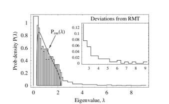
We note the presence of “bulk” (RMT-like) eigenvalues which fall within the bounds [$\lambda_{-},$$\lambda_{+}$] for $P_{rm}\left(\lambda\right)$, and presence of the eigenvalues which lie outside of the “bulk”, representing deviations from the RMT predictions. In particular, largest eigenvalue $\lambda_{497}=8.99$ for seven days period is approximately four times larger than the RMT upper bound $\lambda_{+}$.

The histogram for well-defined bulk agrees with $P_{rm}\left(\lambda\right)$ suggesting that the cross-correlations of matrix $C$ are mostly random. We observe that inter-VLAN traffic time series interact mostly in a random fashion.

Nevertheless, the agreement of empirical probability distribution $P\left(\lambda\right)$ of the bulk with $P_{rm}\left(\lambda\right)$ is not sufficient to claim that the bulk of eigenvalue spectrum is random. Therefore, further RMT tests are needed [19].

To do that, we obtained the unfolded eigenvalues $\xi_{i}$ by following the phenomenological procedure referred to as Gaussian broadening [27], (see [27, 35, 19, 18]). The empirical cumulative distribution function of eigenvalues $F\left(\lambda\right)$ agrees well with the $F_{av}\left(\lambda\right)$ (see Figure 2), where $\xi_{i}$ obtained with Gaussian broadening procedure with the broadening parameter $a=8$.

Figure 2: The empirical cumulative distribution of $\lambda_{i}$ and unfolded eigenvalues $\xi_{i}\equiv F_{av}\left(\lambda\right)$.

The first independent RMT test is the comparison of the distribution of the nearest-neighbor unfolded eigenvalue spacing $P_{nn}\left(s\right)$, where $s\equiv\xi_{k+1}-\xi_{k}$ with $P_{GOE}\left(s\right)$ [9, 10, 11]. The empirical probability distribution of nearest-neighbor unfolded eigenvalues spacing $P_{nn}\left(s\right)$ and $P_{GOE}\left(s\right)$ are presented in Figure 3. The Gaussian decay of $P_{GOE}\left(s\right)$ for large $s$ suggests that $P_{GOE}\left(s\right)$ “probes” scales only of the order of one eigenvalue spacing. The solid line represents.

Figure 3: Nearest-neighbor spacing distribution $P_{nn}\left(s\right)$ of unfolded eigenvalues $\xi_{i}$ of cross-correlation matrix $C$.

The agreement between empirical probability distribution $P_{nn}\left(s\right)$ and the distribution of nearest-neighbor eigenvalues spacing of the GOE matrices $P_{GOE}\left(s\right)$ testifies that the positions of two adjacent empirical unfolded eigenvalues at the distance $s$ are correlated just as the eigenvalues of the GOE matrices.

Next, we took on the distribution $P_{nnn}\left(s^{\prime}\right)$ of next-nearest-neighbor spacings $s^{\prime}\equiv\xi_{k+2}-\xi_{k}$ between the unfolded eigenvalues. According to [8] this distribution should fit to the distribution of nearest-neighbor spacing of the GSE. We demonstrate this correspondence in Figure 4. The solid line shows $P_{GSE}\left(s\right)$.

Figure 4: Next-nearest-neighbor eigenvalue spacing distribution $P_{nnn}\left(s^{\prime}\right).$

Finally, the long-range two-point eigenvalue correlations were tested. It is known [9, 10, 11], that if eigenvalues are uncorrelated we expect the number variance to scale with $l$, $\Sigma^{2}\sim l$. Meanwhile, when the unfolded eigenvalues of $C$ are correlated, $\Sigma^{2}$ approaches constant value, revealing “spectral rigidity” [9, 10, 11]. In Figure 5, we contrasted Poissonian number variance with the one we observed, and came to the conclusion that eigenvalues belonging to the “bulk” clearly exhibit universal RMT properties. The broadening parameter $a=8$ was used in Gaussian broadening procedure to unfold the eigenvalues $\lambda_{i}$ [27, 35, 19, 18]. The dashed line corresponds to the case of uncorrelated eigenvalues.

Figure 5: Number variance $\Sigma^{2}\left(l\right)$ calculated from the unfolded eigenvalues $\xi_{i}$ of $C$.

These findings show that the system of inter-VLAN traffic has a universal part of eigenvalues spectral correlations, shared by broad class of systems, including chaotic and disordered systems, nuclei, atoms and molecules. Thus it can be concluded, that the bulk eigenvalue statistics of the inter-VLAN traffic cross-correlation matrix $C$ are consistent with those of real symmetric random matrix $R$, given by Eq. (5) [24]. Meantime, the deviations from the RMT contain the information about the system-specific correlations. The next section is entirely devoted to the analysis of the eigenvalues and eigenvectors deviating from the RMT, which signifies the meaningful inter-VLAN traffic interactions.

VI inter-vlan traffic interactions analysis

We overview the points of interest in eigenvectors of inter-VLAN traffic cross-correlation matrix $C$, which are determined according to $Cu^{k}=\lambda_{k}u^{k}$, where $\lambda_{k}$ is $k$-th eigenvalue. Particularly important characteristics of eigenvectors, proven to be useful in physics of disordered conductors is the inverse participation ratio (IPR) (see, for example, Ref. [11]). In such systems, the IPR being a function of an eigenstate (eigenvector) allows to judge and clarify whether the corresponding eigenstate, and therefore electron is extended or localized.

VI-A Inverse participation ratio of eigenvectors components

For our purposes, it is sufficient to know that IPR quantifies the reciprocal of the number of significant components of the eigenvector. For the eigenvector $u^{k}$ it is defined as

$$I^{k}\equiv\sum_{l=1}^{N}\left[u_{l}^{k}\right]^{4},$$ (18)

where $u_{l}^{k}$, $l=1,\dots,497$ are components of the eigenvector $u^{k}$. In particular, the vector with one significant component has $I^{k}=1$, while vector with identical components $u_{l}^{k}=1/\sqrt{N}$ has $I^{k}=1/N$.

Figure 6: Inverse participation ratio as a function of eigenvalue $\lambda$.

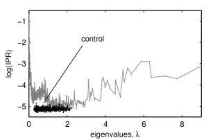
Consequently, the inverse of IPR gives us a number of significant participants of the eigenvector. In Figure 6 we plot the IPR of cross-correlation matrix $C$ as a function of eigenvalue $\lambda$. The control plot is IPR of eigenvectors of random cross-correlation matrix $R$ of Eq. 5. As we can see, eigenvectors corresponding to eigenvalues from $0.25$ to $3.5$, what is within the RMT boundaries, have IPR close to $0$. This means that almost all components of eigenvectors in the bulk interact in a random fashion. The number of significant components of eigenvectors deviating from the RMT is typically twenty times smaller than the one of the eigenvectors within the RMT boundaries, around twenty. For instance, IPR of eigenvector $u^{492}$, which corresponds to the eigenvalue $5.9$ in Figure 6, is $0.05$, i.e. twenty time series are significantly contribute to $u^{492}$. Another observation which we derive from Figure 6 is that the number of eigenvectors significant participants is considerably smaller at both edges of the eigenvalue spectrum. These findings resemble the results of [19], where the eigenvectors with a few participating components were referred to as localized vectors. The theory of localization is explained in the context of random band matrices, where elements independently drawn from different probability distributions [19]. These matrices despite their randomness, still contain probabilistic information. The localization in inter-VLAN traffic is explained as follows. The separated broadcast domains, i.e. VLANs forward traffic from one to another only through the router, reducing the routing for broadcast containment. Although the optimal VLAN deployment is to keep as much traffic as possible from traversing through the router, the bottleneck at the large number of VLANs is unavoidable.

VI-B Distribution of eigenvectors components

Another target of interest is the distribution of the components $\left\{u_{l}^{k};\,l=1,\dots,N\right\}$ of eigenvector $u^{k}$ of the interactions matrix $C$. To calculate vectors $u$ we used the MATLAB routine again and obtained components distribution $p\left(u\right)$ of the eigenvectors components. Then, we contrasted it with the RMT predictions for the eigenvector distribution $p_{rm}\left(u\right)$ of the random correlation matrix $R$. According to [11] $p_{rm}\left(u\right)$ has a Gaussian distribution with mean zero and unit variance, i.e.

$$p_{rm}\left(u\right)=\frac{1}{\sqrt{2\pi}}exp\left(\frac{-u^{2}}{2}\right).$$ (19)

The weights of randomly interacting traffic counts time series, which are represented by the eigenvectors components has to be distributed normally. The results are presented in Figure 7. One can see (from Figures 7a and 7b) that $p\left(u\right)$ for two $u^{k}$ taken from the bulk is in accord with $p_{rm}\left(u\right)$. The distribution $p\left(u\right)$ corresponding to the eigenvalue $\lambda_{i}$, which exceeds the RMT upper bound ($\lambda_{i}>\lambda_{+}$), is shown in Figure 7c. The solid line shows $p_{rm}\left(u\right)$ from Eq. 19. (c) $p\left(u\right)$ for $u^{496}$, corresponding to the eigenvalue outside of the RMT bulk. (d) $p\left(u\right)$ for $u^{497}$, corresponding to largest eigenvalue.

Figure 7: Distribution of components $p\left(u\right)$ of eigenvectors corresponding to eigenvalues (a) from the middle of the bulk, i.e.$\lambda_{-}<\lambda<\lambda_{+}$, (b) from the bulk close to $\lambda_{+}$, (c) $\lambda_{496}$ (d) $\lambda_{497}$.

VI-C Deviating eigenvalues and significant inter-VLAN traffic series contributing to the deviating eigenvectors.

The distribution of $u^{497}$, the eigenvector corresponding to the largest eigenvalue $\lambda_{497}$, deviates significantly from the Gaussian (as follows from Figure 7d). While Gaussian kurtosis has the value 3, the kurtosis of $p\left(u^{497}\right)$ comes out to $23.22$. The smaller number of significant components of the eigenvector also influences the difference between Gaussian distribution and empirical distribution of eigenvector components. More than half of $u^{497}$components have the same sign, thus slightly shifting the $p\left(u\right)$ to one side. This result suggests the existence of the common VLAN traffic intended for inter-VLAN communication that affects all of the significant participants of the eigenvector $u^{497}$with the same bias. We know that the number of significant components of $u^{497}$ is twenty two, since IPR of $u^{497}$is $0.045$. Hence, the largest eigenvector content reveals 22 traffic time series, which are affected by the same event. We obtain the time series, which affects 22 traffic time series by the following procedure. First of all, we calculate projection $G^{497}\left(t\right)$ of the time series $G_{i}\left(t\right)$ on the eigenvector $u^{497}$,

$$G^{497}\left(t\right)\equiv\sum_{i=1}^{497}u_{i}^{497}G_{i}\left(t\right)$$ (20)

Next, we compare $G^{497}\left(t\right)$ with $G_{i}\left(t\right)$, by finding the correlation coefficient $\left\langle\frac{G^{497}\left(t\right)}{\sigma^{497}}\frac{G_{i}\left(t\right)}{\sigma_{i}}\right\rangle$. The Fiber Distributed Data Interface (FDDI)-VLAN internet switch at one of the routers demonstrates the largest correlation coefficient of $0.89$ (see Figure 8).

Figure 8: (a) FDDI-VLAN internet switch time series regressed against the projection $G^{497}\left(t\right)$ from Eq. 20. (b) Time series defined by the eigenvector corresponding to eigenvalue within RMT bounds shows no linear dependence on $G^{497}\left(t\right).$

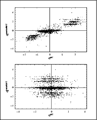
The eigenvector $u^{497}$ has the following content: seven most significant participants are seven FDDI-VLAN switches at the seven routers. The presence of FDDI-VLAN switch provide us with information about VLAN membership definition. FDDI is layer 2 protocol, which means that at least one of two layer 2 membership is used, port group or/and MAC address membership. The next group of significant participants comprises of VLAN traffic intended for routing and already routed traffic from different VLANs. The final group of significant participants constitutes open switches, which pick up any “leaking” traffic on the router. Usually, the “leaking” traffic is the network management traffic, a very low level traffic which spikes when queried by the management systems.

If every deviating eigenvalue notifies a particular sub-model of non-random interactions of the network, then every corresponding eigenvector presents the number of significant dimensions of sub-model. Thus, we can think of every deviating eigenvector as a representative network-wide “snapshot” of interactions within the certain dimensions.

The analysis of the significant participants of the deviating eigenvectors revealed three types of inter-VLAN traffic time series groupings. One group contains time series, which are interlinked on the router. We recognize them as, router1-VLAN_1000 traffic, router1-firewall traffic and VLAN_1000-router1 traffic. The time series, which are listed as router1-vlan_2000, router2-VLAN_2000, router3-VLAN_2000, etc., are reserved for the same service VLAN on every router and comprise another group. The content of these groups suggests the VLANs implementation, it is a mixture of infrastructural approach, where functional groups (departments, schools, etc.) are considered, and service approach, where VLAN provides a particular service (network management, firewall, etc.).

VII stability of inter-vlan traffic interactions in time

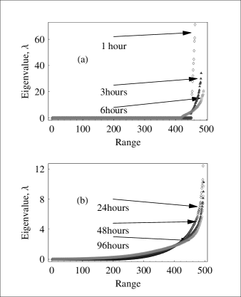
We expect to observe the stability of inter-VLAN traffic interactions in the period of time used to compute traffic cross-correlation matrix $C$. The eigenvalues distribution at different time periods provides the information about the system stabilization, i.e. about the time after which the fluctuations of eigenvalues are not significant. Time periods of $1$ hour, $3$ hours and $6$ hours are not sufficient to gain the knowledge about the system, which is demonstrated in Figure 9a. In Figure 9b the system stabilizes after $1$ day period. To observe the time stability of inter-VLAN meaningful interactions we computed the “overlap matrix” of the deviating eigenvectors for the time period $t$ and deviating eigenvectors for the time period $t+\tau$, where $t=60h,\tau=\left\{0h,3h,12h,24h,36h,48h\right\}$.

Figure 9: (a) Eigenvalues distributions of traffic streams correlation matrix $C$ for $1$ hour, $3$ hours and $6$ hours time intervals. (b) Eigenvalues distributions for $24$ hours, $48$ hours and $72$ hours

First, we obtained matrix D from $p=57$ eigenvectors, which correspond to $p$ eigenvalues outside of the RMT upper bound $\lambda_{+}$. Then we computed the “overlap matrix” $O\left(t,\tau\right)$ from $D_{A}D_{B}^{T}$, where $O_{ij}$ is a scalar product of the eigenvector $u^{i}$ of period $A$ (starting at time $t=t$) with $\textrm{u}^{j}$ of period $B$ at the time $t=t+\tau$,

$$O_{ij}\left(t,\tau\right)\equiv\sum_{k=1}^{N}D_{ik}\left(t\right)D_{ik}\left(t+\tau\right)$$ (21)

The values of $O_{ij}\left(t,\tau\right)$ elements at $i=j$, i.e. of diagonal elements of matrix $O$ will be $1$, if the matrix $D\left(t+\tau\right)$ is identical to the matrix $D\left(t\right)$. Clearly, the diagonal of the “overlap matrix” $O$ can serve as an indicator of time stability of $p$ eigenvectors outside of the RMT upper bound $\lambda_{+}$. The gray scale colormap of the “overlap matrices” $O\left(t=60h,\tau=\left\{0h,3h,12h,24h,36h,48h\right\}\right)$ is presented in Figure 10. Black color of grayscale represents $O_{ij}=1$, white color represents $O_{ij}=0.$ The most stable eigenvalue is $\lambda_{492}.$

Figure 10: The grayscale of overlap matrix $O\left(t,\tau\right)$ at $t=60h$ and $\tau=\left\{0h,3h,12h,24h,36h,48h\right\}$.

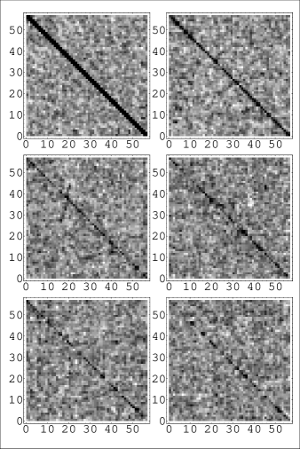
At lag $\tau=3$ hours the inter-VLAN interactions show the highest degree of stability. For further lags the overall stability decays. As the analysis of deviating eigenvectors content showed, the highly interacting traffic time series are time series of service based VLANs, intended for routing. Particular network services are evoked at the same time and active for the same period of time, which explains the stability and consequent decay of deviating eigenvectors of traffic interactions.

VIII detecting anomalies of traffic interactions

We assume that the health of inter-VLAN traffic is expressed by stability of its interactions in time. Meanwhile, the temporal critical events or anomalies will cause the temporal instabilities. The “deviating” eigenvalues and eigenvectors provide us with stable in time snapshots of interactions representative of the entire network. Therefore, these eigenvectors judged on the basis of their IPR can serve as monitoring parameters of the system stability.

Among the essential anomalous events of VLAN infrastructure we can list violations in VLAN membership assignment, in address resolution protocol, in VLAN trunking protocol, router misconfiguration. The violation of membership assignment and router misconfiguration will cause the changes in the picture of random and non-random interactions of inter-VLAN traffic. To shed more light on the possibilities of anomaly detection we conducted the experiments to establish spatial-temporal traces of instabilities caused by artificial and temporal increase of the correlation in normal non-congested inter-VLAN traffic. We explored the possibility to distinguish different types of increased temporal correlations. Finally, we observed the consequences of breaking the interactions between time series, by injecting traffic counts obtained from sample of random distribution.

Experiment 1

We selected the traffic counts time series representing the components of the eigenvector which lies within the RMT bounds and temporarily increased the correlation between these series for three hour period. The proposed monitoring parameters show the dependence of system stability on the number of temporarily correlated time series (see Figure 11). Presented in Figure 11, left to right are (a) eigenvalue distribution of interactions with two temporarily correlated time series, (b) IPR of eigenvectors of interactions with two temporarily correlated time series, (c) the overlap matrix of deviating eigenvectors with two temporarily correlated time series. Top to bottom the layout shows these monitoring parameters when correlation is temporarily increased between 10 connections (d,e and f) and between 20 connections (g,h and i).

Figure 11: Eigenvalues distribution, IPR and overlap matrix of deviating eigenvectors.

One can conclude that increased temporal correlation between two time series and between ten time series does not affect system stability. Meanwhile, when the number of temporarily correlated time series reaches the number of significant participants of $u^{497},$ which is calculated as inverse of $I^{497}$and is equal to twenty two, the system becomes visibly unstable. The largest eigenvalue changes from $10$ in stable condition to $12$, the tail of inverse participation ratio plot is extended and the diagonal of “overlap matrix” disappears at twenty temporarily correlated time series.

In Figures 12 (a, b, c and d ), the temporal correlation between ten time series is traced with the matrix of sorted in decreasing order of their components deviating from RMT eigenvectors.

Figure 12: Sorted deviating eigenvectors with injected correlation among ten traffic time series.

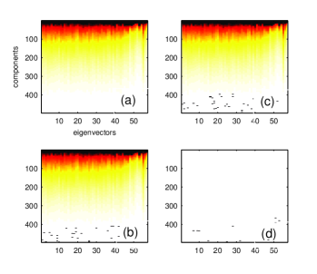
The sorted in decreasing order deviating eigenvectors of $60h$ of uninterrupted traffic are presented in Figure 12a. Then, after three hours of uninterrupted traffic the weights of eigenvectors components, which had zero value start changing, This is captured in Figure 12b. Same process for traffic with induced three hours correlation is captured in Figure 12c. The difference between results in Figures 12b and 12c is presented in Figure 12d. The procedure used to visualize this produces the high rate of false positive alarms.

In addition, we visualize in Figure 13 the system instability during temporal increase of correlation between twenty time series with spatial-temporal representation of eigenvector $u^{497}$.

Figure 13: (a) The weights of components of $u^{497}$ plotted for time period from $36$ to $84$ hours of uninterrupted traffic with 6 hours interval. (b) The weights of components of $u^{497}$ plotted with respect to the same time period, with induced three hours correlation. (c) The weights of components of $u^{496}$ plotted with respect to the same time period, with induced three hours correlation.

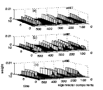
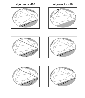
We used the weights of components of eigenvector $u^{497}$, defined for IPR computation and plotted them with respect to time $t+\tau$, where $t=36$ hours and $\tau=6n,$ where $n\in\left\{0,1,\dots,7\right\}$. In Figure 13a the spatial-temporal pattern of $u^{497}$ captures precise locations of system-specific interactions of uninterrupted traffic for $84$ hours of observation. The abrupt change of this pattern in Figure 13b indicates the starting point of induced correlation between twenty traffic time series usually interacting in a random fashion. It turns out, that the “normal” stable pattern of eigenvector $u^{497}$ moves to eigenvector $u^{496}$, when the interruption ends. Thus, we are able to observe the end point of the induced correlations in Figure 13c, which represents weights of components of eigenvector $u^{496}$ plotted with respect to the same time intervals. With this setup we are able to locate the anomaly in time and space. Translated to network topological representation, the behavior of eigenvectors $u^{497}$and $u^{496}$ during our manipulations with inter-VLAN traffic may be monitored with the following graphs (see Figure 14).

Figure 14: Left column - behavior of $u^{497}$ during time period from $48$h to $60$h with $6$h time window, induced correlation starts at $54$h and lasts for $3$h. Right column - behavior of $u^{496}$ in same conditions.

Experiment 2

In the previous experiment we injected just one type of increased correlation among time series. Now we make two and three different types of induced correlations produce different spatial-temporal patterns on eigenvector $u^{497}$ components (see Figure 15). Time series for temporal increase of correlation are obtained in the same way as in Experiment 1. We temporarily increased the correlation between series by inducing elements from distributions of sine function and quadratic function, respectively for three hours.

Figure 15: (a) The weights of components of $u^{497}$ plotted for time period from $36$ to $84$ hours with $6$ hours interval, two different types of induced correlations. (b) The weights of components of $u^{497}$ plotted with respect to the same time period, three different types of induced correlations.

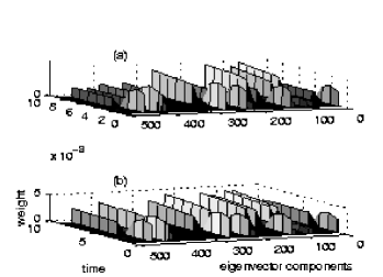
In Figure 15a, one type of three hours correlation is induced among ten traffic time series and another type of correlation among other ten time series. Three different types of three hours correlations are induced among twenty traffic time series in Figure 15b. The sorted in decreasing order content of significant components shows that time series tend to group according to the type of correlation they are involved in.

Experiment 3

Next we turn our attention to disruption of normal picture of inter-VLAN traffic interactions. This can be done by injecting the traffic from random distribution to non-randomly interacting time series for three hours. We demonstrate it by examining the eigenvalue distribution, the IPR and the deviating eigenvectors overlap matrix plotted in Figure 16.

Figure 16: Eigenvalues distribution, IPR and overlap matrix of deviating eigenvectors of inter-VLAN traffic cross-correlation matrix $C$.

After $60$ hours of uninterrupted traffic, we injected elements from random distribution to significant participants of $u^{497}$ for three hours. The largest eigenvalue increases, from $10$ to $12.$ Extended IPR tail shows the larger number of localized eigenvectors and we observe the dramatic break in deviating eigenvectors stability.

IX conclusion and future work

The RMT methodology we used in this paper enables us to analyze the complex system behavior without the consideration of system constraints, type and structure. Our goal was to investigate the characteristics of day-to-day temporal dynamics of the system of interconnected routers with VLAN subnets of the University of Louisville. The type and structure of the system at hand suggests the natural interpretation of the RMT-like behavior and the RMT deviating results. The time stable random interactions signify the healthy, and free of congestion traffic. The time stable non-random interactions provide us with information about large-scale network-wide traffic interactions. The changes in the stable picture of random and non-random interactions signify the temporal traffic anomalies.

In general, the fact of sharing the universal properties of the bulk of eigenvalues spectrum of inter-VLAN traffic interactions with random matrices opens a new venue in network-wide traffic modeling. As stated in [19], in physical systems it is common to start with the model of dynamics of the system. This way, one would model the traffic time series interactions with the family of stochastic differential equations [28, 29], which describe the “instantaneous” traffic counts

$$g_{i}\left(t\right)=\left(d/dt\right)lnT_{i}\left(t\right),$$ (22)

as a random walk with couplings. Then one would relate the revealed interactions to the correlated “modes” of the system.

Additional question that RMT findings raise in network-wide traffic analysis is whether the found eigenvalues spectrum correlations and localized eigenvectors outside of RMT bulk can add to the explanation of the fundamental property of the network traffic, such as self-similarity [30].

To summarize, we have tested the eigenvalues statistics of inter-VLAN traffic cross-correlation matrix $C$ against the null hypothesis of random correlation matrix. By separating the eigenvalues spectrum correlations of random matrices that are present in this system, the uncongested state of the network traffic is verified. We analyzed the stable in time system-specific correlations. The analyzed eigenvalues and eigenvectors deviating from the RMT showed the principal groups of VLAN-router switches, groups of traffic time series interlinked through the firewalls and groups of same service VLANs at every router. With straightforward experiments on the traffic time series, we demonstrated that eigenvalue distribution, IPR of eigenvectors, overlap matrix and spatial-temporal patterns of deviating eigenvectors can monitor the stability of inter-VLAN traffic interactions, detect and spot in time and space of any network-wide changes in normal traffic time series interactions.

As the reservation for the future work, we would like to investigate the behavior of delayed traffic time series cross-correlation matrix $C_{d}$ in the RMT terms. The importance of delay in measurement-based analysis of Internet is emphasized in [31]. To understand and quantify the effect of one time series on another at a later time, one can calculate the delay correlation matrix, where the entries are cross-correlation of one time series and another at a time delay $\tau$ [32]. In addition, we are interested in testing the fruitfulness of the RMT approach on the larger system of inter-domain interactions, for instance, on 5-minute averaged traffic count time series of underlying backbone circuits of Abilene backbone network.

Appendix A RMT

In this Appendix, we provide a short (and non-rigorous) explanation of main concepts and glossary of terms used in the RMT studies. The RMT approaches, which originated in nuclear and condensed matter physics and later became common in many branches of mathematical physics [25], have recently penetrated into econophysics, finance [26] and network traffic analysis [3].

For the statistical description of complex physical systems, such as, for example, atomic nucleus or acoustical reverberant structure, the RMT serves as guiding light when one is interested in the degree of mutual interaction of the constituents. As it turns out, the uncorrelated energy levels or acoustic eigenfrequencies would produce qualitatively different result from those obeying RMT-like correlations [25]. Therefore, real (experimentally measured) spectra can help to decide on the nature of interactions in the underlying system. To be specific, ideally, symmetric system is expected to exhibit spectral properties drastically different from the properties of generic one, and if the spectral properties are those of RMT systems, other ideas of RMT can be brought to the researcher aid.

To describe “awareness” of the structural constituents about each other, scientists in different fields use similar constructs. Physicists use Hamiltonian matrix, engineers stiffness matrix, finance and network analysts the equal-time cross-correlation matrix. Although the physical meaning of mentioned operators can be different, the eigenvalues/eigenvectors analysis seems to be a universally accepted tool. The eigenvalues have direct connection to spectrum of physical systems, while eigenvectors can be used for the description of excitation/signal/information propagation inside the system. In physics, the RMT approaches come about whenever the system of interest demonstrates certain qualitative features in their spectral behavior. For example, if one looks at nearest neighbor spacing distribution of eigenvalues and instead of Poisson law

$$P\left(s\right)=\exp\left(-s\right),$$

discovers “Wigner surmise”

$$P\left(s\right)=\frac{\pi}{2}s\exp\left(-\frac{\pi}{2}s^{2}\right),$$

one concludes (upon running several additional statistical tests) that apparatus of RMT can be used for the system at hand, and system matrix can be replaced by a matrix with random entries. For mathematical convenience, these entries are given Gaussian weight. The only other ingredient of this rather succinct phenomenological model is recognizing the physical situation. For example, systems with and without magnetic field and/or central symmetry are described by different matrix ensembles (that is the set of matrices) with elements distributed within distribution corresponding to the same $\beta$

$$P^{\left(\beta\right)}\left(H\right)\propto\textrm{exp}\left(-\frac{\beta}{4v^{2}}trH^{2}\right),$$

where the constant $v$ sets the length of the resulting eigenvalues spectrum.

The very fact that RMT can be helpful in statistical description of the broad range of systems suggests that these systems are analyzed in a certain special universal regime, in which physical or other laws are undermined by equilibrated and ergodic evolution. In most physical applications, a Hamiltonian matrix is rather sparse, indicating lack of interaction between different subparts of the corresponding object. However, if the universal regime is inferred from the above mentioned statistical tests, it is very beneficial to replace this single matrix with the ensemble of random matrices. Then, one can proceed with statistical analysis using matrix ensemble for calculation of statistical averages more relevant for the physical problem at hand than the statistics of eigenvalues. The latter can be mean or variance of the response to external or internal excitation.

References

- [1] K. Fukuda, PhD Thesis: A study on phase transition phenomena in internet traffic, Keio University, 1999.
- [2] T. Ohira, R. Sawatari, Phase transition in a computer network traffic model, Phys. Rev. E 58, July 1998, 193-195.
- [3] M. Barthelemy, B. Gondran and E. Guichard, Large scale cross-correlations in internet traffic, arXiv:cond0mat/0206185 vol 2 3 Dec 2002.
- [4] A. Lakhina, M. Crovella, and C. Diot, Detecting distributed attacks using network-wide flow traffic, Proceedings of FloCon 2005 Analysis Workshop, 2005.
- [5] A. Lakhina, M. Crovella, and C. Diot. Mining Anomalies Using Traffic Feature Distributions. Technical Report BUCS-TR-2005-002, Boston University, 2005.
- [6] E.P. Wigner, On a class of analytic functions from the quantum theory of collisions, Ann. Math. 53, 36 (1951), Proc. Cambridge Philos. Soc. 47, 790 (1951).
- [7] F. Dyson, Statistical theory of the energy levels of complex systems, J. Math. Phys. 3, 140 (1962).
- [8] F. Dyson and M.L. Mehta, Statistical theory of the energy levels of complex systems, J. Math. Phys. 4, 701, 713 (1963).
- [9] M.L Mehta, Random matrices (Academic Press, Boston, 1991).
- [10] T.A. Brody, J.Flores, J.B. French, P.A. Mello, A. Pandey, and S.S.M. Wong, Random-matrix physics: spectrum and strength fluctuations, Rev. Mod. Phys. 53, 385 - 479, issue 3, July 1981.
- [11] T. Guhr, A. Muller-Groeling, and H.A. Weidenmuller, Random matrix theories in quantum physics: common concepts, Phys. Rep. 299, 190 (1998).
- [12] M. Krbalek and P.Seba, Statistical properties of the city transport in Cuernavaca (Mexico) and random matrix theory. J. Phys. 214 (2000), 1, 91-100.
- [13] J. McNutt and M. De Shon, Correlation between quiescent ports in network flows, CERT network situational awareness group report, Carnegie Mellon University, September 2005.
- [14] A. Lakhina, M. Crovella, and C. Diot, Characterization of network-wide anomalies in traffic flows, Proceedings of the ACM/SIGCOMM Internet Measurement conference, 2004, 201-206.
- [15] L. Min, Y. Shun-Zheng, A network-wide traffic anomaly detection method based on HSMM, Int. conf. on communications, circuits and system proceedings, vol 6, June 2006, 1636 - 1640.
- [16] M. Roughan, T. Griffin, M. Mao, A. Greenberg, and B. Freeman, Combining routing and traffic data for detection of IP forwarding anomalies, Proceedings of the joint int. conf. on Measurement and modeling of computer systems, 2004, 416 - 417.
- [17] L. Huang, X. Nguyen, M. Garofalakis, M. Jordan, A. Joseph and N. Taft, Distributed PCA and network anomaly detection, Technical report No. UCB/EECS-2006-99.
- [18] S. Sharifi, M. Crane, A. Shamaie and H. Ruskin, Random matrix portfolio optimization: a stability approach, Physica A 335 (2004) 629-643.
- [19] V. Plerou, P. Gopikrishnan, B. Rosenow, L. A. Nunes Amaral, T. Guhr, and H.E. Stanley, Random matrix theory approach to cross correlations in financial data, Phys. Rev. E, vol 65, 066126, 27 June 2002.
- [20] A. Tulino and S. Verdu, Random matrix theory and wireless communications, Communications and Information theory, vol 1, issue 1, June 2004, 1 - 182.
- [21] D. Tse, Multiuser receivers, random matrices and free probability, Proceedings of 37th Ann. Allerton Conf., Monticello, IL, September 1999.
- [22] A. Zee, Random matrix theory and RNA folding, Acta Physica Polonica B, vol 36, No 9, June 2005.
- [23] L. Laloux, P. Cizeau, J.-P. Bouchaud, and M. Potters, Noise dressing of financial correlation matrices, Phys. Rev. Lett. 83, August 1999, 1467-1470.
- [24] A.M. Sengupta and P.P. Mitra, Distributions of singular values for some random matrices, arXiv:cond-mat/9709283 vol 1 25 September 1997.
- [25] H.-J. Stockman, Quantum Chaos: an introduction, 1999.
- [26] J.-P. Bouchaud, Theory of financial risk and derivative pricing: from statistical physics to risk management, 1962.
- [27] H. Bruus and J.-C. Angles d’Auriac, Energy level statistics of two-dimensional Hubbard model at low filling, arXiv:cond-mat/9610142 vol 1 18 October 1996.
- [28] J.D. Farmer, Market Force, ecology and evolution, e-print adap-org/9812005, Int. J. Theo. Appl. fin. 3, 425, 2000.
- [29] J.-P. Bouchaud, R. Cont, A Langevin approach to stock market fluctuations and crashes, European Journal of Physics, B 6, 543, 1998.
- [30] W.E. Leland, M.S. Taqq, W. Willinger, and D.V. Willson, On the self-similar nature of Ethernet traffic, ACM SIGCOMM, 1993, 183 - 193.
- [31] B. Zhang, T.S. Eugene Ng, and A. Nandi, Measurement-based analysis, modeling, and synthesis of the Internet delay space, Proceedings of the 6-th ACM SIGCOMM on Internet Measurement, 2006, 85-98.
- [32] K.B.K. Mayya and R.E. Amritkar, Analysis of delay correlation matrices, oai:arXiv.org:cond-mat/0601279 (2006-12-20).
- [33] W.-C. Lau, S.-Q. Li, Traffic analysis in large-scale high-speed integrated networks:validation of nodal decomposition approach, INFOCOM, 1993, Proceedings of twelfth annual joint conference of the IEEE Computer and Communications Societies, vol 3, 1320-1329.
- [34] W.H. Allen, G.A. Marin, L.A. Rivera, Automated detection of malicious reconnaissance to enhance network security, SoutheastCon, 2005, Proceedings of IEEE, issue 8-10, April 2005, 450-454.
- [35] H. Bruus and J.-C. Angles d’Auriac, The spectrum of two-dimensional Hubbard model at low filling, Europhysics letters, 35 (5), 321-326, 1999.