Intrinsic Spin Hall Effect: Topological Transitions in Two-Dimensional Systems

Abstract

The spin-Hall conductivity in spatially-homogeneous two-dimensional electron systems described by the spin-orbit Hamiltonian $\hbar\mbox{\boldmath$\Omega$}_{\bf p}\cdot\hat{\mbox{\boldmath$\sigma$}}$ is presented as a sum of the universal part $Me/8\pi\hbar$ determined by the Berry phase $\Phi=M\pi$ ($M$ is an odd integer, the winding number of the vector $\mbox{\boldmath$\Omega$}_{\bf p}$) and a non-universal part which vanishes under certain conditions determined by the analytical properties of $\mbox{\boldmath$\Omega$}_{\bf p}$. The analysis reveals a rich and complicated behavior of the spin-Hall conductivity which is relevant to both electron and hole states in quantum wells and can be detected in experiments.

Owing to the spin-orbit interaction (SOI), an electric field applied along two-dimensional (2D) electron layers can generate transverse spin currents in the absence of external magnetic fields. This phenomenon, known as the spin Hall effect [1], is at the focus of attention in modern physics. The presence of SOI terms in the Hamiltonian of free electrons leads to the intrinsic spin-Hall conductivity expressed in the universal units $e/\hbar$ in the case of weak disorder. The original theoretical proposal [2] of the universal intrinsic spin Hall effect has been based on the Rashba Hamiltonian [3] describing the linear in 2D momentum ${\bf p}=(p_{x},p_{y})$ spin-orbit coupling due to structural inversion asymmetry. However, numerous theoretical calculations [4-8] have proved the absence of static intrinsic spin currents for this case. As follows from the equation of motion for the spin density operator [9], this statement is applicable to any electron system described by a ${\bf p}$-linear SOI Hamiltonian. The situation is quite different in the case of 2D hole systems described by the effective ${\bf p}$-cubic SOI Hamiltonian [10] $h^{(3)}_{\bf p}=\hbar\kappa(\hat{\sigma}_{+}p_{-}^{3}+\hat{\sigma}_{-}p_{+}^{3})$, where $\hat{\sigma}_{\pm}=(\hat{\sigma}_{x}\pm i\hat{\sigma}_{y})/2$, $\hat{\sigma}_{\alpha}$ are the Pauli matrices, and $p_{\pm}=p_{x}\pm ip_{y}$. Theoretical studies [11-15] based upon this Hamiltonian have confirmed the existence of the intrinsic spin Hall effect. The experimentally observed spin Hall effect in 2D hole systems [16,17] is likely of the intrinsic origin.

What makes the systems described by the Hamiltonian $h^{(3)}_{\bf p}$ so different from the systems described by p-linear SOI Hamiltonians? It is the dependence of SOI on the angle $\varphi$ of the 2D momentum. This dependence is characterized by the odd integers known as the winding numbers (WN), which are equal to $\pm 3$ and $\pm 1$ for the ${\bf p}$-cubic and ${\bf p}$-linear Hamiltonians considered above. In 2D hole systems, owing to the increased WN, the conservation of the spin density is no longer reduced to the requirement of zero spin currents, so the intrinsic spin Hall effect exists. The role of WN in spin response can be also emphasized by considering their influence on the collision-mediated spin-charge coupling term known from the Kubo formalism as the vertex correction [4]. If the scattering is symmetric (caused by the short-range potential), the vertex correction for the WN $\pm 3$ is zero, since it is given by the angular average of the product of the charge current operator by the SOI Hamiltonian. In contrast, for ${\bf p}$-linear SOI the vertex correction is always nonzero and leads to nonexistence of spin currents.

It is important to realize that the consideration of SOI Hamiltonians containing the terms with WN either $\pm 1$ or $\pm 3$ is not sufficient for description of the spin response in 2D systems. The coexistence of SOI terms with WN $\pm 1$ and $\pm 3$ in semiconductor quantum wells is rather a rule than an exception. For example, this is the case of conduction-band electrons in the quantum wells made of noncentrosymmetric semiconductors [18] at high electron densities, when both ${\bf p}$-linear and ${\bf p}$-cubic Dresselhaus terms are important. The aim of this Letter is to find out the general properties of the intrinsic spin currents for the systems described by the SOI Hamiltonians containing an arbitrary mixture of terms with different WN and to establish relevance of such a consideration to both electron and hole states in quantum wells.

The starting point is the free-electron Hamiltonian in the momentum representation:

$$\hat{H}_{\bf p}=\varepsilon_{p}+\hat{h}_{\bf p},~{}~{}~{}\hat{h}_{\bf p}=\hbar\mbox{\boldmath$\Omega$}_{\bf p}\cdot\hat{\mbox{\boldmath$\sigma$}},$$ (1)

where $\varepsilon_{p}$ is the kinetic energy (isotropic but not necessarily parabolic) and $\mbox{\boldmath$\Omega$}_{\bf p}$ is an arbitrary vector antisymmetric in momentum. The $2\times 2$ matrix SOI term $\hat{h}_{\bf p}$ describes both 2D electrons and 2D holes (since the 4-fold degeneracy of the $\Gamma_{8}$ valence band is lifted in quantum wells, the 2D holes are quasiparticles with two spin states). The calculations are based on the quantum kinetic equation for the Wigner distribution function [19] which is a $2\times 2$ matrix over the spin indices. Searching for the linear response to the applied electric field ${\bf E}$ in the stationary and spatially homogeneous case, one can write the distribution function in the form $\hat{f}^{(eq)}_{\mathbf{p}}+\hat{f}_{\mathbf{p}}$, where $\hat{f}_{\mathbf{p}}$ is the non-equilibrium part satisfying the linearized kinetic equation

$$\frac{i}{\hbar}\left[\hat{h}_{\mathbf{p}},\hat{f}_{\mathbf{p}}\right]+e{\bf E}\cdot\frac{\partial\hat{f}^{(eq)}_{\mathbf{p}}}{\partial{\bf p}}=\widehat{J}(\hat{f}|\mathbf{p}).$$ (2)

The collision integral $\widehat{J}$ describes the elastic scattering, and the spin-orbit corrections [1] to the scattering potential are neglected. Considering this integral in the Markovian approximation and assuming that $\hbar\Omega_{\bf p}\equiv\hbar|{\mbox{\boldmath$\Omega$}_{\bf p}}|$ is small in comparison to the mean kinetic energy, one can expand $\widehat{J}$ in series of $\Omega_{\bf p}$ [14,19]. Using the spin-vector representation $\hat{f}_{\bf p}={\rm f}^{0}_{\bf p}+\hat{\mbox{\boldmath$\sigma$}}\cdot{\rm{\bf f}}_{\bf p}$, one gets

$$-2[\mbox{\boldmath$\Omega$}_{\bf p}\times{\rm{\bf f}}_{\bf p}]+{\bf A}_{\bf p}=\frac{m_{p}}{\hbar^{3}}\int_{0}^{2\pi}\!\!\frac{d\varphi^{\prime}}{2\pi}w_{|{\bf p}-{\bf p}^{\prime}|}({\rm{\bf f}}_{\bf p^{\prime}}-{\rm{\bf f}}_{\bf p}),$$ (3)

where $w_{q}$ is the Fourier transform of the correlator of the scattering potential, $|{\bf p}^{\prime}|=|{\bf p}|$ is assumed, and $\varphi^{\prime}$ is the angle of the vector ${\bf p}^{\prime}$. Next, ${\bf A}_{\bf p}$ is a vector proportional to ${\bf E}$, and $m_{p}\equiv\frac{1}{2}(\partial p^{2}/\partial\varepsilon_{p})$ is the $p$-dependent effective mass as it enters the expression for the group velocity, ${\bf v}_{\bf p}=\partial\varepsilon_{p}/\partial{\bf p}={\bf p}/m_{p}$. Analytical solution of Eq. (3) is possible for short-range scattering potential, when $w_{|{\bf p}-{\bf p}^{\prime}|}\simeq w$. Then the right-hand side of Eq. (3) is written as $\nu_{p}(\overline{{\rm{\bf f}}}_{\bf p}-{\rm{\bf f}}_{\bf p})$, where $\nu_{p}=m_{p}w/\hbar^{3}$ is the scattering rate and the line over a function denotes the angular averaging. Also,

$$\frac{A^{\alpha}_{\bf p}}{\hbar e}={\bf E}\cdot\!\frac{\partial({\bf v}_{\bf p}\Omega^{\alpha}_{\bf p}-\overline{{\bf v}_{\bf p}\Omega^{\alpha}_{\bf p}})f^{\prime}_{\varepsilon_{p}}}{\partial\varepsilon_{p}}+[{\bf E}\times{\bf n}]\cdot\frac{f^{\prime}_{\varepsilon_{p}}}{p^{2}}\frac{\partial{\bf p}\Omega^{\alpha}_{\bf p}}{\partial\varphi},$$ (4)

where $f^{\prime}_{\varepsilon_{p}}\equiv\partial f_{\varepsilon_{p}}/\partial\varepsilon_{p}$ is the derivative of the Fermi distribution function $f_{\varepsilon}$, and ${\bf n}$ is the unit vector normal to the quantum well plane. Notice the property $\overline{A^{\alpha}_{\bf p}}=0$.

Solution of Eq. (3) determines the non-equilibrium spin current density ${\bf q}_{\gamma}=\frac{1}{2}\int\frac{d{\bf p}}{(2\pi\hbar)^{2}}{\rm Tr}(\{\hat{\mbox{\boldmath$\sigma$}},\hat{u}_{\gamma}({\bf p})\}\hat{f}_{\bf p})$, where $\hat{u}_{\gamma}({\bf p})=\partial(\varepsilon_{p}+\hat{h}_{\bf p})/\partial p_{\gamma}$ is the group velocity in the presence of spin-orbit interaction, $\{~{},~{}\}$ denotes the symmetrized matrix product, and ${\rm Tr}$ is the matrix trace. The spin conductivity is introduced according to ${\bf q}_{\gamma}=\mbox{\boldmath$\Sigma$}_{\gamma\beta}E_{\beta}$. Based on Eqs. (3) and (4),

$$\mbox{\boldmath$\Sigma$}_{\gamma\beta}=-\frac{e}{8\pi\hbar}\int d\varepsilon_{p}~{}f^{\prime}_{\varepsilon_{p}}\left({\bf T}^{\gamma\beta}_{p}-[\overline{{\bf P}^{\gamma}_{\bf p}}\times{\bf Q}^{\beta}_{p}]\right).$$ (5)

The vector-functions standing here are defined as angular averages: ${\bf T}^{\gamma\beta}_{p}=2\overline{\left[{\bf P}^{\gamma}_{p}\times(\partial\mbox{\boldmath$\Omega$}_{\bf p}/\partial p_{\beta})\right]}$, ${\bf P}^{\gamma}_{\bf p}=p_{\gamma}\mbox{\boldmath$\Omega$}_{\bf p}/\Delta^{2}_{\bf p}$, $\Delta^{2}_{\bf p}=\Omega^{2}_{\bf p}+\nu^{2}_{p}/4$, and ${\bf Q}^{\beta}_{p}=2[\overline{\widehat{R}}_{p}]^{-1}\overline{\widehat{R}_{p}(\partial\mbox{\boldmath$\Omega$}_{\bf p}/\partial p_{\beta})}$, where $\widehat{R}_{p}$ is a symmetric matrix with elements $R^{\alpha\beta}_{p}=(\Omega^{2}_{\bf p}\delta_{\alpha\beta}-\Omega^{\alpha}_{\bf p}\Omega^{\beta}_{\bf p})/\Delta^{2}_{\bf p}$. One can find also the induced spin density: ${\bf s}=\frac{1}{2}\int\frac{d{\bf p}}{(2\pi\hbar)^{2}}{\rm Tr}(\hat{\mbox{\boldmath$\sigma$}}\hat{f}_{\bf p})=(e\hbar^{2}/4\pi w)\int d\varepsilon_{p}f^{\prime}_{\varepsilon_{p}}{\bf Q}^{\beta}_{p}E_{\beta}$. The limit of low temperature [20] is described by the substitution $f^{\prime}_{\varepsilon_{p}}=-\delta(\varepsilon_{p}-\varepsilon_{F})$, so the spin conductivity tensor is expressed directly through the vector-functions taken at the Fermi surface $\varepsilon_{p}=\varepsilon_{p_{F}}=\varepsilon_{F}$.

Equation (5) is valid for arbitrary $\mbox{\boldmath$\Omega$}_{\bf p}$. In the quantum wells grown along [001] direction in cubic crystals of zinc-blende type, the $C_{2v}$ point group symmetry implies

$$\mbox{\boldmath$\Omega$}_{\bf p}=(\Omega^{x}_{\bf p},\Omega^{y}_{\bf p},0),~{}~{}\Omega^{x}_{p,-\pi/4+\varphi}=\Omega^{y}_{p,-\pi/4-\varphi},$$ (6)

where the polar coordinate representation ${\bf p}\equiv(p,\varphi)$ is used. Then ${\bf T}^{\gamma\beta}_{p}=(0,0,T^{\gamma\beta}_{p})$, $\overline{{\bf P}^{\gamma}_{\bf p}}=(P_{p}^{x\gamma},P_{p}^{y\gamma},0)$, and ${\bf Q}^{\beta}_{p}=(Q_{p}^{x\beta},Q_{p}^{y\beta},0)$, where $T^{xx}_{p}=-T^{yy}_{p}$, $T^{xy}_{p}=-T^{yx}_{p}$, $P^{xx}_{p}=-P^{yy}_{p}$, $P^{xy}_{p}=-P^{yx}_{p}$, $Q^{xx}_{p}=-Q^{yy}_{p}$, and $Q^{xy}_{p}=-Q^{yx}_{p}$. The spin currents exist only for $z$-spins, $\mbox{\boldmath$\Sigma$}_{\gamma\beta}=(0,0,\Sigma_{\gamma\beta})$, and there are two independent components $\Sigma_{xy}=-\Sigma_{yx}\equiv\Sigma_{H}$ and $\Sigma_{xx}=-\Sigma_{yy}$ describing spin-Hall and spin-diagonal currents, respectively. The function $T^{xy}_{p}$ entering $\Sigma_{H}$ can be written as

$$T^{xy}_{p}=\int_{0}^{2\pi}\!\!\frac{d\varphi}{2\pi\Delta^{2}_{p,\varphi}}\left(\Omega^{x}_{p,\varphi}\frac{\partial\Omega^{y}_{p,\varphi}}{\partial\varphi}-\Omega^{y}_{p,\varphi}\frac{\partial\Omega^{x}_{p,\varphi}}{\partial\varphi}\right).$$ (7)

In the case of zero temperature, using the notations $T^{xy}\equiv T^{xy}_{p_{F}}$ and $\mbox{\boldmath$\Omega$}_{\varphi}\equiv\mbox{\boldmath$\Omega$}_{p_{F},\varphi}$, it is convenient to write

$$\Sigma_{H}=\frac{e}{8\pi\hbar}T^{xy}+\delta\Sigma_{H},$$ (8)

where $\delta\Sigma_{H}$ expresses the contribution of the second term in Eq. (5). In the collisionless limit, the formal integration in Eq. (7) leads to

$$T^{xy}=\frac{\Phi}{\pi},~{}~{}\Phi=\frac{1}{2}\oint d\arg[\Omega^{+}(z)]=\pi(N_{0}-N_{\infty}),$$ (9)

where $\Omega^{+}(z)=\Omega^{x}_{\varphi}+i\Omega^{y}_{\varphi}$ is a function of the complex variable $z=e^{i\varphi}$, and the contour of integration in the complex plane is the circle of unit radius, $|z|=1$. Next, $N_{0}$ and $N_{\infty}$ are the numbers of zeros and poles of $\Omega^{+}(z)$ inside this circle (it is assumed that $\Omega^{+}(z)$ does not have branch points). Using the conventional definitions (see [21] and references therein) it is easy to identify $\Phi$ with the Berry phase in the momentum space. In the WN representation, the function $\Omega^{+}(z)$ is a polynomial containing odd powers of $z$, in the general case, from $z^{-N}$ to $z^{N}$, assuming that the highest WN involved in $\mbox{\boldmath$\Omega$}_{\bf p}$ is $N$. Then $N_{\infty}=L$, where $L\leq N$ is an odd integer (the order of the multiple pole at $z=0$), while $N_{0}$ takes even values from $0$ to $L+M$, where $-L\leq M\leq N$ depending on the SOI parameters. Therefore, if $\Omega_{\bf p}$ contains an arbitrary mixture of terms with different WN up to $N$, the spin-Hall conductivity is

$$\Sigma_{H}=\frac{Me}{8\pi\hbar}+\delta\Sigma_{H},~{}~{}~{}|M|=1,3,\ldots,N,$$ (10)

where $M=N_{0}-N_{\infty}$ is the acting WN, which describes the actual winding of the vector $\mbox{\boldmath$\Omega$}_{\bf p}$ as ${\bf p}$ goes around the Fermi surface, and can be found, in each concrete case, from the simple analysis explained above. The corresponding Berry phase is $\pi M$. The spin-Hall conductivity changes abruptly when the functions $\Omega^{x}_{\varphi}$ and $\Omega^{y}_{\varphi}$ go through zero simultaneously at certain angles $\varphi$. In other words, each time when the SOI parameters are adjusted in such a way that the spin splitting $2\hbar\Omega_{\bf p}$ at the Fermi surface becomes zero at certain ${\bf p}$, a topological transition occurs: the Berry phase changes by $\pm 2\pi$. For the Hamiltonians with $N=1$ including both Rashba and Dresselhaus (linear) terms, this effect has been studied in the Berry phase approach in Refs. 21-23. In this particular case, however, the first term in Eq. (10) is exactly compensated by the second term, and $\Sigma_{H}=0$. Therefore, the topological transitions essentially require the SOI with WN greater than unity.

The result (10) is exact in the collisionless limit and can be viewed as a quantization of the spin-Hall conductivity in terms of the WN. In general, this quantization does not occur in integer numbers of $e/4\pi\hbar$, because $\delta\Sigma_{H}$ is also a discontinuous function of SOI parameters and undergoes abrupt changes together with the first term in Eq. (10). To show this, it is sufficient to represent $P^{\alpha\gamma}$ as combinations of the integrals $\oint dz[\Omega^{+}(z)]^{-1}$, $\oint dz[z^{2}\Omega^{+}(z)]^{-1}$, and complex conjugate terms. It is important that such a representation allows one to find the general conditions for vanishing $\delta\Sigma_{H}$: this takes place when either a) all zeros of $\Omega^{+}(z)$ are inside the circle $|z|=1$ and $N_{0}-N_{\infty}\geq 3$ or b) the order of the multiple pole at $z=0$ is $L\geq 3$ and all zeros of $\Omega^{+}(z)$ (if present) are outside the circle $|z|=1$. In particular, this means that if the highest WN involved in $\mbox{\boldmath$\Omega$}_{\bf p}$ is, in the same time, the acting WN ($M=N$ or $M=-N$ at $N\neq 1$), the spin-Hall conductivity stays at the universal value $Me/8\pi\hbar$ without regard to the SOI parameters. If $N\geq 5$, $\Sigma_{H}$ can take universal values from $\pm 3e/8\pi\hbar$ to $\pm Ne/8\pi\hbar$.

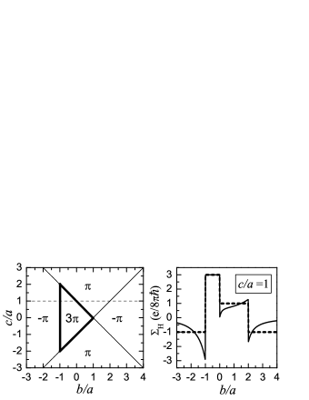
Figure 1: Left: Phase diagram for the SOI of Eq. (11) at $u_{p}=0$. The regions of fixed Berry phase $\Phi$ (indicated) are separated by the lines of topological transitions (solid). Right: Spin-Hall conductivity $\Sigma_{H}$ (solid) and its universal part (dash) as functions of $b/a$ at $c/a=1$. It is assumed that $\partial\ln|b_{p}|/\partial\ln p=\partial\ln|c_{p}|/\partial\ln p=\!1$ and $\partial\ln|a_{p}|/\partial\ln p=\!3$.

The most general form of $\mbox{\boldmath$\Omega$}_{\bf p}$ including WN $\pm 1$ and $\pm 3$ for [001]-grown quantum wells is

$$\Omega^{x}_{\bf p}=c_{p}\sin\varphi-b_{p}\cos\varphi-u_{p}\sin 3\varphi-a_{p}\cos 3\varphi,$$

$$\Omega^{y}_{\bf p}=-c_{p}\cos\varphi+b_{p}\sin\varphi-u_{p}\cos 3\varphi-a_{p}\sin 3\varphi.$$ (11)

This form describes both electron and hole states. For conduction-band electrons, there are the Rashba ($c_{p}$) and the Dresselhaus ($b_{p}$) terms, while the $a_{p}$-term exists because of the ${\bf p}$-cubic Dresselhaus contribution. The $u_{p}$-term can be attributed to higher-order invariants allowed by symmetry. For holes in the ground-state subband, the $a_{p}$- and $b_{p}$-terms exist due to the structural inversion asymmetry. The term containing $a_{p}\propto p^{3}$ is the one considered in the theory of the spin Hall effect for holes, this term is derived [10] from the isotropic Luttinger Hamiltonian. The anisotropy of the Luttinger Hamiltonian, described by the parameter $\mu=(\gamma_{2}-\gamma_{3})/(\gamma_{2}+\gamma_{3})$, where $\gamma_{i}$ are the Luttinger parameters in their usual notations, leads to the $b_{p}$-term with $b_{p}=\mu a_{p}$. Next, the $c_{p}$- and $u_{p}$-terms for holes are caused by the bulk inversion asymmetry [24]. The $c_{p}$-term includes the contribution $\alpha_{h}p$ proportional to $p$ [24,25], which should dominate at low hole densities. In the general case, especially when the structural asymmetry is weak, an adequate description of hole states should include all terms in Eq. (11).

Figure 2: Spin-Hall conductivity as a function of density in electron (a) and hole (b) systems. The dashed lines correspond to the collisionless approximation, $\nu=0$. The solid lines are plotted for $\nu=0.2\beta(\pi\hbar/d)$ (a) and for $\nu=0.5|\alpha_{h}^{3}/\kappa|^{1/2}$ (b).

The simplest case of the SOI with combined WN described by Eq. (11) is realized when $c_{p}=u_{p}=0$. One finds the analytical expression

$$\Sigma_{H}=\frac{e}{8\pi\hbar}\frac{a^{2}+b^{2}-r^{2}}{2b^{2}r^{2}}\left[(3-\eta)(a^{2}-b^{2})+\eta r^{2}\right],$$ (12)

where $r_{p}^{2}=\sqrt{[(a_{p}+b_{p})^{2}\!+\!\nu_{p}^{2}/4][(a_{p}-b_{p})^{2}\!+\!\nu_{p}^{2}/4]}-\!\nu_{p}^{2}/4$, $\eta_{p}=1/2+(1/4)\partial\ln|b_{p}/a_{p}|/\partial\ln p$, and all coefficients are taken at $p=p_{F}$. According to the Berry phase analysis, $\Sigma_{H}=3e/8\pi\hbar$ at $|a|>|b|$ in the collisionless limit, while Eq. (12) gives

$$\Sigma_{H}=\frac{3e}{8\pi\hbar}\times\left\{\begin{array}[]{l}1,\\ -(1-2\eta/3)(a/b)^{2},\end{array}\begin{array}[]{c}a^{2}>b^{2}\\ a^{2}<b^{2}\end{array}\right..$$ (13)

In application to conduction-band electrons, when the Dresselhaus model implies $a_{p}=\lambda p^{3}$, $b_{p}=\beta p-\lambda p^{3}$, and $\lambda\simeq\beta(d/2\pi\hbar)^{2}$ (for a deep square well of width $d$), this means that $\Sigma_{H}$ abruptly jumps to the universal value $3e/8\pi\hbar$ if the electron density $n_{2D}=p_{F}^{2}/2\pi\hbar^{2}$ increases and exceeds $\pi/d^{2}$. A similar behavior, though without a qualitative explanation, has been found in Ref. 26. For holes, $a_{p}=-\kappa p^{3}$, $b_{p}=-\mu\kappa p^{3}$, and $|a|>|b|$ since $|\mu|<1$. This means that $\Sigma_{H}$ of 2D holes in [001]-grown wells is insensitive to the anisotropy of the Luttinger Hamiltonian and stays at the universal value for the case of clean hole systems.

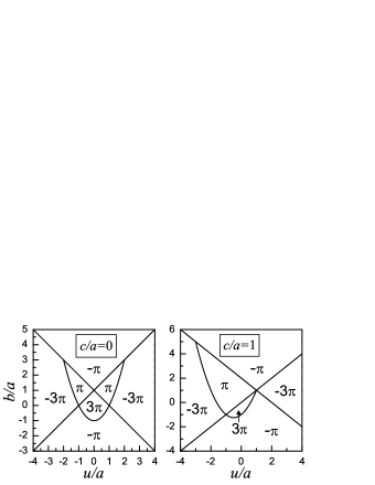
Figure 3: Phase diagrams for the SOI of Eq. (11). The Berry phases $\Phi$ for each region are indicated. The spin-Hall conductivity is $\pm 3e/8\pi\hbar$ in the regions with $\Phi=\pm 3\pi$.

If the $c_{p}$-term is added into consideration, the analysis leads to the phase diagram shown in Fig. 1. The spin-Hall conductivity is equal to $3e/8\pi\hbar$ at $-1<b/a<1-|c/a|$, in the region inside the bold triangle in Fig. 1. There are 5 regions, and several topological transitions can take place as the parameters are varied. To demonstrate a possibility of their experimental observation, one should put $c_{p}=\alpha p$ for electrons and $c_{p}=\alpha_{h}p$ for holes. The Rashba coefficient $\alpha$ is determined by structural asymmetry, while $\alpha_{h}\simeq 2\delta\alpha_{v}/(\hbar d)^{2}$ [24], where $\delta\alpha_{v}=-0.035$ eV nm³ for GaAs. The results of calculations are shown in Fig. 2. For electrons, $\Sigma_{H}$ is plotted as a function of the dimensionless parameter $2d^{2}n_{2D}/\pi=(p_{F}d/\pi\hbar)^{2}$ in the range $p_{F}<\sqrt{3}\pi\hbar/d$, when only the lowest electron subband in the deep square well is populated. If Rashba coupling is nonzero, this dependence has two jumps and the region of universal behavior is shifted towards higher densities. If $|\alpha/\beta|$ exceeds 1, $\Sigma_{H}$ becomes considerably suppressed in the chosen density range. For holes, it is convenient to use the dimensionless units $2\pi\hbar^{2}|\kappa/\alpha_{h}|n_{2D}=|a/c|$. The transition takes place at $|a/c|=1/(1-\mu)$. Estimating $\hbar^{4}\kappa\sim 0.1$ eV nm³ from the data of Ref. 17 and assuming $d\simeq 5$ nm, one finds that this condition corresponds to $n_{2D}\sim 5\times 10^{11}$ cm^-2, so the transition occurs at a reasonable density and can be observed experimentally. Instead of varying $n_{2D}$, it is possible to change $\alpha$ for electrons and $\kappa$ for holes by biasing the structure.

Finally, after adding the $u_{p}$-term the phase diagram becomes more complicated, it is described in terms of three variables, $c/a$, $b/a$, and $u/a$. Figure 3 shows two sections of this three-dimensional phase diagram, which demonstrate coexistence of the regions with $\Phi=3\pi$ and $\Phi=-3\pi$, and a possibility of transitions between them, when $\Sigma_{H}$ changes by $3e/4\pi\hbar$. The regions of $\Phi=-3\pi$ exist when $|u/a|>1$. If $|c/a|>3$, the region of $\Phi=3\pi$ disappears.

In conclusion, the presence of SOI terms with different angular dependences and interference of these terms in the spin response makes the physics of the spin Hall effect more rich than it is usually assumed. The consideration given above is an attempt to plot a map to this new world, only part of which has been investigated so far.

References

(1)
H.-A. Engel, E. I. Rashba, and B. I. Halperin, Theory of Spin Hall Effects in
Semiconductors (Contribution to the Handbook of Magnetism and Advanced Magnetic
Materials, Vol. 5, Wiley, 2007) [cond-mat/0603306].
(2)
J. Sinova, D. Culcer, Q. Niu, N. A. Sinitsyn, T. Jungwirth, and A. H. MacDonald,
Phys. Rev. Lett. 92, 126603 (2004).
(3)
Y. A. Bychkov and E. I. Rashba, J. Phys. C 17, 6039 (1984).
(4)
J. I. Inoue, G. E. W. Bauer, and L. W. Molenkamp, Phys. Rev. B 70, 041303(R) (2004).
(5)
E. G. Mishchenko, A. V. Shytov, and B. I. Halperin, Phys. Rev. Lett. 93,
226602 (2004).
(6)
O. V. Dimitrova, Phys. Rev. B 71, 245327 (2005).
(7)
O. Chalaev and D. Loss, Phys. Rev. B 71, 245318 (2005).
(8)
A. Khaetskii, Phys. Rev. Lett. 96, 056602 (2006).
(9) K. Nomura, J. Sinova, N. A. Sinitsyn, and A. H. MacDonald,
Phys. Rev. B 72, 165316 (2005).
(10) R. Winkler, H. Noh, E. Tutuc, and M. Shayegan, Phys. Rev. B
65, 155303 (2002).
(11) J. Schliemann and D. Loss, Phys. Rev. B 71, 085308 (2005).
(12) S. Y. Liu and X. L. Lei, Phys. Rev. B 72, 155314 (2005).
(13) B. A. Bernevig and S.-C. Zhang, Phys. Rev. Lett. 95, 016801 (2005).
(14) A. V. Shytov, E. G. Mishchenko, H.-A. Engel, and B. I. Halperin,
Phys. Rev. B 73, 075316 (2006).
(15) A. Khaetskii, Phys. Rev. B 73, 115323 (2006).
(16) J. Wunderlich, B. Kaestner, J. Sinova, and T. Jungwirth,
Phys. Rev. Lett. 94, 047204 (2005).
(17) K. Nomura, J. Wunderlich, J. Sinova, B. Kaestner, A. H. MacDonald,
and T. Jungwirth, Phys. Rev. B 72, 245330 (2005).
(18) R. Eppenga and M. F. H. Schuurmans, Phys. Rev. B 37, 10923 (1988).
(19) F. T. Vasko and O. E. Raichev, Quantum Kinetic Theory and
Applications (Springer, New York, 2005).
(20) A. G. Mal’shukov, L. Y. Wang, C. S. Chu, and K. A. Chao, Phys. Rev. Lett.
95, 146601 (2005).
(21) S.-Q. Shen, Phys. Rev. B 70, 081311(R) (2004).
(22) T.-W. Chen, C.-M. Huang, and G. Y. Guo, Phys. Rev. B 73, 235309 (2006).
(23) R. Raimondi, C. Gorini, P. Schwab, and M. Dzierzawa,
Phys. Rev. B 74, 035340 (2006).
(24) E. I. Rashba and E. Ya. Sherman, Phys. Lett. A 129, 175 (1988).
(25) R. Winkler, Phys. Rev. B 62, 4245 (2000).
(26) A. G. Mal’shukov and K. A. Chao, Phys. Rev. B 71, 121308(R) (2005).