On invariant $2\times 2$ $\beta$-ensembles of random matrices.

Abstract

We introduce and solve exactly a family of invariant $2\times 2$ random matrices, depending on one parameter $\eta$, and we show that rotational invariance and real Dyson index $\beta$ are not incompatible properties. The probability density for the entries contains a weight function and a multiple trace-trace interaction term, which corresponds to the representation of the Vandermonde-squared coupling on the basis of power sums. As a result, the effective Dyson index $\beta_{\mathrm{eff}}$ of the ensemble can take any real value in an interval. Two weight functions (Gaussian and non-Gaussian) are explored in detail and the connections with $\beta$-ensembles of Dumitriu-Edelman and the so-called Poisson-Wigner crossover for the level spacing are respectively highlighted. A curious spectral twinning between ensembles of different symmetry classes is unveiled: as a consequence, the identification between symmetry group (orthogonal, unitary or symplectic) and the exponent of the Vandermonde ($\beta=1,2,4$) is shown to be potentially deceptive. The proposed technical tool more generically allows for designing actual matrix models which i) are rotationally invariant; ii) have a real Dyson index $\beta_{\mathrm{eff}}$; iii) have a pre-assigned confining potential or alternatively level-spacing profile. The analytical results have been checked through numerical simulations with an excellent agreement. Eventually, we discuss possible generalizations and further directions of research.

1 Introduction.

Ensembles of matrices with random elements have been widely studied since the pioneering works of Wigner Wigner and Dyson Dys:new on the ’threefold way’. A first, gross classification of random matrix (RM) models can take into account i) whether the size $N$ of the matrices in the ensemble is finite or the limit $N\rightarrow\infty$ is taken and ii) whether the probability distribution of the entries remains invariant after a rotation in the matrix space.

The requirement of rotational invariance implies that the joint probability density (jpd) of the eigenvalues can be written as:

$$P(\lambda_{1},\ldots,\lambda_{N})\propto e^{-\frac{1}{2}\sum_{i=1}^{N}V(\lambda_{i})}\prod_{j<k}|\lambda_{j}-\lambda_{k}|^{\beta}$$ (1)

where $V(x)$ is a confining potential ($x^{2}$ for Gaussian ensembles) and the interaction term between eigenvalues is the well-known Vandermonde determinant raised to the power $\beta$. The Dyson index $\beta$ can classically take only the values $1,2,4$ according to the number of variables needed to specify a single entry ($1$ for real, $2$ for complex and $4$ for quaternion numbers). This $\beta$ index in turn identifies the symmetry group of the ensemble (Orthogonal, Unitary and Symplectic respectively).

Thanks to the works of Mehta Mehta and many others, very powerful analytical tools are available to deal with invariant ensembles, both for finite $N$ and as $N\rightarrow\infty$, the latter limit being usually the most interesting for RM theorists. However, it was very soon realized that matrices with the smallest size $N=2$ can equally well provide deep insights and trigger new ideas, the most successful one being the celebrated Wigner’s surmise Mehta which gives an excellent approximation for the level spacing of bigger matrices. The study of $2\times 2$ random matrices has since been strongly developed and it remains an active area of research in mathematical physics caurier lenz chau ahmed araujo kota ahmed2 jackson evangelou sabbah ullah2 alhassid shaffaf vanassche .

The purpose of the present paper is to introduce and solve exactly a family of $2\times 2$ random matrices depending on one parameter $\eta$. This ensemble will have rotational invariance but a real effective Dyson index $\beta_{\mathrm{eff}}$ in an interval. Although it is commonly assumed that the two properties:

• rotational invariance;

• real Dyson index.

are essentially incompatible, since the Dyson index of an invariant ensemble is strictly constrained to the values $1,2$ or $4$ as described above, we will show how to construct explicitly a counterexample in Section 2 introducing suitable correlations among the matrix entries. The motivation for this study stems from two apparently unrelated issues, namely the Dumitriu-Edelman $\beta$-ensembles DE and the so-called Poisson-Wigner crossover for the level spacing BohLes . In order to make the paper self-contained, we give a brief introduction to both of them highlighting also the two main tasks we tackle in this paper. In subsection 1.3, we provide the plan of the article.

1.1 $\beta$-ensembles of Dumitriu-Edelman.

Consider the jpd (1). Does there exist a non-trivial matrix model having (1) as its jpd of eigenvalues for any $\beta>0$? Very recently, Dumitriu and Edelman were able to answer this question affirmatively DE . They introduced two ensembles of tridiagonal $N\times N$ matrices with independent entries, whose jpd of eigenvalues is exactly given by (1) for general $\beta>0$ DE . These ensembles have been called $\beta$-Hermite and $\beta$-Laguerre, according to the classical weight their jpd contains. This result is essential for an efficient numerical sampling of random matrices vivo and has triggered a significant amount of further research dumitriu forrRain killip lippert esutton .

Note that the $\beta$-ensembles, having independent non-Gaussian entries are obviously non-invariant. Thus, the first novel task we tackle in this paper (Section 3) is the following:

Task 1

Design and solve exactly a $(2\times 2)$ ensemble with:

• rotational invariance;

• running $\beta_{\mathrm{eff}}\geq 0$ ;

• assigned classical potential (in particular, Gaussian-Hermite).

In fact, an invariant matrix model displaying a running Dyson index would be of great interest: tuning the strength of the correlations between the eigenvalues in (1) has significant importance for systems which, although endowed with an intrinsic invariance, are subjected to a weak non-invariant perturbation (see e.g. zyc ) and may also have important implications for lattice gas theory bakerforr . Furthermore, it is a long-standing observation that nuclear systems with two-body interactions display an average density of states whose profile is much closer to a Gaussian distribution bohigas french than to a semicircle. Hence, a RM approach with the appropriate symmetries clearly requires much weaker, and possibly suppressed altogether, correlations among the energy levels than those arising from (1) with integer and fixed $\beta$. In this respect, the limit $\beta_{\mathrm{eff}}\rightarrow 0$ of our model is particularly appealing (see Section 3).

1.2 Poisson-Wigner crossover.

Another interesting transitional regime in quantum chaos theory, namely the so-called Poisson-Wigner crossover for level spacings, has attracted much attention in the past twenty years BohLes . In terms of the dimensionless nearest-neighbor spacing $s$, the Poisson and Wigner distributions are given by:

$$P_{\mathrm{POI}}(s) =\exp(-s)$$ (2)

$$P_{\mathrm{WIG}}(s) =\frac{\pi s}{2}\exp\left(-\frac{\pi s^{2}}{4}\right)$$ (3)

and correspond to the limiting cases of classical dynamics, namely purely regular and completely chaotic. Intermediate regimes between those two extremes have been intensely investigated (see guhr for a review), and interpolating phenomenological formulas have been proposed, the most famous being the Brody brody and Berry-Robnik berry distributions. The quest for a deeper understanding of such a crossover has motivated many proposals of parametrical random matrix models whose level spacing distribution interpolates between (2) and (3) cheon ullah pato caurier lenz chau . Normally, the requirement of rotational invariance is the first to be dropped in those models. The reason is easy to understand: once this condition is imposed, the Vandermonde-coupling between the eigenvalues forces the level spacing $P(s)$ to display a term of the form $\sim s^{\beta}$ ($\beta=1,2,4$) and thus is very stiff, at least for small values of the gap $s$. No meaningful crossover could occur in such models for any standard choice of the confining potential. This problem would be overcome by an invariant model with a tunable index $\beta_{\mathrm{eff}}$ and thus leads to our second unconventional task (Section 4):

Task 2

Design and solve exactly a $(2\times 2)$ ensemble with:

• rotational invariance;

• running $\beta_{\mathrm{eff}}\geq 0$;

• assigned level-spacing profile.

1.3 Plan of the paper.

The $2\times 2$ ensemble we are going to introduce in Section 2 is completely defined when one assigns:

• A symmetry group (SG) (Orthogonal, Unitary or Symplectic), corresponding to real symmetric, hermitian or quaternion self-dual matrices;

• A weight function, to be defined in Section 2;

• A range for the free parameter $\eta$.

As far as the SG is concerned, in the present study we will confine ourselves to hermitian (unitary invariant) matrices, although generalizations to other SG may be easily derived (see Section 5). The Dyson index for this Unitary ensemble turns out to be $\beta_{\mathrm{eff}}=\beta-2\eta=2-2\eta$ and for this reason we call the ensemble $\eta$-UE ($\eta$-Unitary Ensemble).

In Sections 3 and 4 we make two different choices for the combination (weight function $+$ range for $\eta$) in order to tackle the tasks 1 and 2 described above. More precisely:

• Section 3: choosing as an example a standard Gaussian potential, we design a $\eta$-UE ensemble which is essentially a $(2\times 2)$ $\beta$-Hermite model DE plus rotational invariance for $\eta\in[0,1]$. We compute analytically the marginal distributions of the correlated entries in subsection 3.1 and we derive explicitly the spectral properties in 3.2. These results are then checked by numerical diagonalization of actual $\eta$-UE samples in subsection 3.3.

• Section 4: choosing as limiting cases the Wigner and the Poisson level-spacing profile, we design a $\eta$-UE ensemble whose level spacing interpolates between the two cases for the parameter $\eta\in[1/2,1]$. Following the same guidelines, it is in principle possible to extend the analysis to an arbitrary pre-assigned level-spacing profile $\tilde{P}_{\eta}(s)$.

In Section 5 we discuss generalizations of this model towards different SG, different weight functions and extended ranges for $\eta$. At that stage, we will make comments about some emerging features of our model that appear interesting to be tackled in future researches.
In Section 6, we first provide a synthetic table with a comparison of the main features of all the ensembles considered in this work, and then we add some concluding remarks. Some technical derivations are also given in the Appendices.

2 Main idea and the model.

Let $\mathbf{P}_{\eta}[\mathcal{X}]\equiv\mathbf{P}_{\eta}(x_{11},\ldots,x_{NN})$ be the joint probability density of the entries for a $N\times N$ random matrix ensemble, depending on the parameter $\eta$. If the model is required to be rotationally invariant, as in our case, two facts must be taken into account:

1. Weyl’s Lemma holds Mehta , so $\mathbf{P}_{\eta}[\mathcal{X}]$ can be only a function of the traces of the first $N$ powers of $\mathcal{X}$. We highlight this point by writing hereafter starred quantities (such as $\mathbf{P}_{\eta}^{\star}:=\mathbf{P}_{\eta}[\mathcal{X}]$) whenever they are meant to be written in terms of traces of powers of $\mathcal{X}$.

2. the jpd of eigenvalues is given by:

   $$P_{\eta}(\lambda_{1},\ldots,\lambda_{N})\propto\mathbf{P}_{\eta}^{\star}\times\prod_{j<k}|\lambda_{j}-\lambda_{k}|^{\beta}$$ (4)

   where the Vandermonde term comes from integrating out the ‘angular’ variables in the diagonalization $\mathcal{X}\rightarrow O\Lambda O^{-1}$. In (4), the $\beta$ index can take only the values $1,2$ or $4$ according to the SG of the ensemble (Orthogonal, Unitary or Symplectic respectively).

We can specialize the properties 1 and 4 to an ensemble of $2\times 2$ unitary invariant hermitian matrices:

$$\mathcal{X}=\begin{pmatrix}x&\frac{t+is}{\sqrt{2}}\\ \frac{t-is}{\sqrt{2}}&y\\ \end{pmatrix}$$ (5)

where $x,y,t,s$ are random variables taken from a jpd $\mathbf{P}_{\eta}(x,y,t,s)$ and the $1/\sqrt{2}$ factors are included for later convenience.

In this simplified case, (4) becomes:

$$P_{\eta}(\lambda_{1},\lambda_{2})\propto\mathbf{P}_{\eta}^{\star}\times|\lambda_{2}-\lambda_{1}|^{2}$$ (6)

and we choose to write the $\eta$-UE jpd of entries as:

$$\mathbf{P}_{\eta}^{\star}:=\frac{\mathcal{W}^{\star}_{\eta}}{[\mathcal{V}^{\star}]^{\eta}}$$ (7)

In (7), the weight function $\mathcal{W}^{\star}_{\eta}$ is a non-negative, normalizable and symmetric function of the eigenvalues, expressed in terms of the traces $(\mathrm{Tr}\mathcal{X},\mathrm{Tr}\mathcal{X}^{2})$. It may depend or not on the parameter $\eta<3/2$.

Now, we define:

$$\mathcal{V}^{\star}=2\mathrm{Tr}\mathcal{X}^{2}-(\mathrm{Tr}\mathcal{X})^{2}$$ (8)

and it is easy to prove the following identity involving the rhs of (8):

$$2\mathrm{Tr}\mathcal{X}^{2}-(\mathrm{Tr}\mathcal{X})^{2}=|\lambda_{2}-\lambda_{1}|^{2}$$ (9)

Through (9), the Vandermonde-squared coupling has been represented in terms of traces of powers of $\mathcal{X}$ and the jpd of eigenvalues (6) becomes:

$$P_{\eta}(\lambda_{1},\lambda_{2})\propto\mathcal{W}_{\eta}^{\star}\times|\lambda_{2}-\lambda_{1}|^{2-2\eta}$$ (10)

As $\eta\in\mathcal{I}\subset\mathbb{R}$, the effective Dyson index $\beta_{\mathrm{eff}}=2-2\eta$ assumes real values in an interval, while the ensemble keeps its rotational invariance (unlike in the case of $\beta$-ensembles of Dumitriu-Edelman). The price to pay is that the entries are no longer independent, but get correlated through the multiple trace-trace interaction term $\mathcal{V}^{\star}$.

One may ask whether the crucial identity (9) is just an algebraic accident holding only for $2\times 2$ matrices or it has a deeper origin. In fact, (9) turns out to be a special case of the more general identity:

$$\prod_{j<k}(\lambda_{j}-\lambda_{k})^{2} =\det\mathcal{\mathbf{M}}_{N}[\mathcal{X}_{N}]=$$

$$=\left|\begin{array}[]{ccccc}N&s_{1}&s_{2}&\cdots&s_{N-1}\\ s_{1}&s_{2}&s_{3}&\cdots&s_{N}\\ s_{2}&s_{3}&s_{4}&\cdots&s_{N+1}\\ \vdots&\vdots&&\ddots&\\ s_{N-1}&s_{N}&s_{N+1}&\cdots&s_{2(N-1)}\end{array}\right|$$ (16)

where $s_{k}=\mathrm{Tr}\mathcal{X}_{N}^{k}$ dunne . Since the Vandermonde-squared coupling is a symmetric polynomial in the eigenvalues, it can be represented on the basis of power sums macdonald , which are nothing but traces of higher order powers of $\mathcal{X}_{N}$. The representation (2) precisely encodes this change of basis, which is currently used in the context of the fractional quantum Hall effect but usually overlooked in RM studies. Note that the general expansion (2) can be used in principle to define a $N\times N$ $\eta$-UE model, although any analytical approach appears very challenging in this case.

From (10), it is clear that different choices for the weight function and the range $\mathcal{I}$ for $\eta$ can be combined to achieve a variety of results. In particular, we are now ready to tackle the first task described in the Introduction.

3 First Task: Gaussian weight function.

Suppose we choose the confining potential to be harmonic $V(x)=x^{2}$. It is then sufficient to make the simple choices $\mathcal{W}_{\eta}^{\star}=\exp\left(-\frac{1}{2}\mathrm{Tr}\mathcal{X}^{2}\right)$ and $\eta\in[0,1]$ to design a $\beta_{\mathrm{eff}}$-Hermite model ($\beta_{\mathrm{eff}}\in[0,2]$) DE plus unitary invariance which we are going to solve exactly. Before doing that, we make the following important remark:

Remark 1

Unlike in the case of $\beta$-Hermite ensemble, the value $\beta_{\mathrm{eff}}\equiv 0$ can be actually reached in $\eta$-UE for $\eta=1$. This corresponds to independent normally distributed eigenvalues.

From (7) and (8) we get:

$$\mathbf{P}_{\eta}^{\star}=\mathrm{C}_{\eta}\frac{e^{-\frac{1}{2}\mathrm{Tr}\mathcal{X}^{2}}}{[2\mathrm{Tr}\mathcal{X}^{2}-(\mathrm{Tr}\mathcal{X})^{2}]^{\eta}}$$ (17)

where $\mathrm{C}_{\eta}$ is a normalization constant.

The resulting jpd of eigenvalues (6) can be written as:

$$P_{\eta}(\lambda_{1},\lambda_{2})=\mathrm{K}_{\eta}e^{-\frac{1}{2}(\lambda_{1}^{2}+\lambda_{2}^{2})}|\lambda_{2}-\lambda_{1}|^{2-2\eta}$$ (18)

where the normalization constant is given by DE :

$$\mathrm{K}_{\eta}=\left(\sqrt{\pi}\,2^{3-2\eta}\,\Gamma\left(\frac{3}{2}-\eta\right)\right)^{-1}$$ (19)

Note that (18) is almost equivalent to a $2\times 2$ $\beta_{\mathrm{eff}}$-Hermite jpd (apart from the actual $\beta_{\mathrm{eff}}=0$ case which is not included there), although the underlying matrix model is very different in the two cases. For a related model with complex eigenvalues, see callaway .

The range of variability for $\eta$ is largely arbitrary (see also subsection 5.3). The choice of $[0;1]$ is motivated by a nice duality between the limiting cases $\eta=0$ and $\eta=1$ as in the following table:

	$\eta=0$	$\eta=1$
Correlation among Eigenvalues	Strong	Absent
Correlation among Entries	Absent	Strong

Table 1: The jpd of entries factorizes for $\eta=0$ and gives rise to GUE (Gaussian Unitary Ensemble) with strongly correlated eigenvalues. On the contrary, for $\eta=1$ the jpd of eigenvalues factorizes and the eigenvalues become i.i.d. normal variables, while the entries are strongly correlated.

Although (17) defines completely our $\eta$-UE model, it is instructive to compute analytically the marginal distributions for the set of correlated variables $(x,y,t,s)$ for two reasons:

1. These results are numerically implemented in subsection 3.3 to generate and diagonalize actual samples of $\eta$-UE matrices. The numerical results will be compared with the spectral properties derived in subsection 3.2.

2. The marginal distributions deviate smoothly from the GUE factorized marginals as $\eta$ departs from zero, and thus they provide quantitative information about the onset of correlations between the entries.

3.1 Marginal distribution of entries.

From (5) one has:

$$\mathrm{Tr}\mathcal{X} =x+y$$ (20)

$$\mathrm{Tr}\mathcal{X}^{2} =x^{2}+y^{2}+t^{2}+s^{2}$$ (21)

so that (17) implies:

$$\mathbf{P}_{\eta}(x,y,t,s):=\mathrm{C}_{\eta}\frac{e^{-\frac{1}{2}(x^{2}+y^{2}+t^{2}+s^{2})}}{[2(x^{2}+y^{2}+t^{2}+s^{2})-(x+y)^{2}]^{\eta}}$$ (22)

The first task is computing the normalization constant $\mathrm{C}_{\eta}$, for which the following integral is needed [GR formula 3.382(4)]:

$$\mathcal{I}(\eta,\ell):=\int_{0}^{\infty}\frac{re^{-\frac{1}{2}r^{2}}}{[2r^{2}+\ell^{2}]^{\eta}}dr=2^{-2\eta}e^{\ell^{2}/4}\Gamma\left(1-\eta,\frac{\ell^{2}}{4}\right)$$ (23)

where $\Gamma(x,y)$ is the incomplete Gamma function.

The constant $\mathrm{C}_{\eta}^{-1}$ is given by:

$$\mathrm{C}_{\eta}^{-1}=\int_{-\infty}^{\infty}\cdots\int_{-\infty}^{\infty}\frac{dx~{}dy~{}dt~{}ds~{}e^{-\frac{1}{2}(x^{2}+y^{2}+t^{2}+s^{2})}}{[2(x^{2}+y^{2}+t^{2}+s^{2})-(x+y)^{2}]^{\eta}}$$ (24)

which becomes upon the change to polar coordinates $(t,s)\rightarrow(r,\theta)$:

$$\mathrm{C}_{\eta}^{-1}=2\pi\int_{-\infty}^{\infty}\int_{-\infty}^{\infty}dx~{}dy~{}e^{-\frac{1}{2}(x^{2}+y^{2})}\mathcal{I}(\eta,x-y)$$ (25)

After further simplifications and the change of variables $(x+y,x-y)\rightarrow(\phi,\omega)$ the double integral decouples and we get:

$$\mathrm{C}_{\eta}^{-1}=\pi^{3/2}2^{3-2\eta}\Gamma\left(\frac{3}{2}-\eta\right)$$ (26)

Now, we can compute the marginal distribution for the variable $x$ following essentially the same steps (hereafter we use the notation $\mathbf{p}_{k,\eta}$ with $k=1,2,3$ to denote the marginals with $k$ variables):

$$\mathbf{p}_{1,\eta} (x)=\mathrm{C}_{\eta}\int_{-\infty}^{\infty}\cdots\int_{-\infty}^{\infty}dy~{}dt~{}ds~{}\mathbf{P}_{\eta}(x,y,t,s)=$$

$$=2\pi\mathrm{C}_{\eta}\frac{d}{dx}\int_{0}^{x}d\mu\int_{-\infty}^{\infty}dy~{}e^{-\frac{1}{2}(\mu^{2}+y^{2})}\mathcal{I}(\eta,y-\mu)=$$

$$=2^{2-2\eta}\pi\mathrm{C}_{\eta}\frac{d}{dx}\int_{-\infty}^{\infty}d\omega\Gamma(1-\eta,\omega^{2})\int_{\omega}^{\omega+x}d\phi e^{-\phi^{2}}=$$

$$=2^{2-2\eta}\pi\mathrm{C_{\eta}}\int_{-\infty}^{\infty}d\omega\Gamma(1-\eta,\omega^{2})e^{-(x+\omega)^{2}}=$$

$$=\frac{\left(f_{\eta}\ast g\right)(x)}{2\sqrt{\pi}\Gamma\left(\frac{3}{2}-\eta\right)}$$ (27)

where in the last passage we have employed the symmetry $\omega\rightarrow-\omega$ of the integral and the convolution $(\ast)$ is between the functions:

$$f_{\eta}(y):=\Gamma(1-\eta,y^{2})\qquad g(y):=e^{-y^{2}}$$ (28)

In the limiting case $\eta\rightarrow 0$, we expect to recover the pure GUE marginal distribution for the entry $x$, which is simply a standard Gaussian. Taken into account that $f_{\eta=0}(y)=g(y)$ and $\Gamma(3/2)=\sqrt{\pi}/2$, one gets:

$$\mathbf{p}_{1,\eta=0}(x)=\frac{1}{\pi}\int_{-\infty}^{\infty}d\omega e^{-\omega^{2}}e^{-(x-\omega)^{2}}=\frac{e^{-x^{2}/2}}{\sqrt{2\pi}}$$ (29)

as it should.

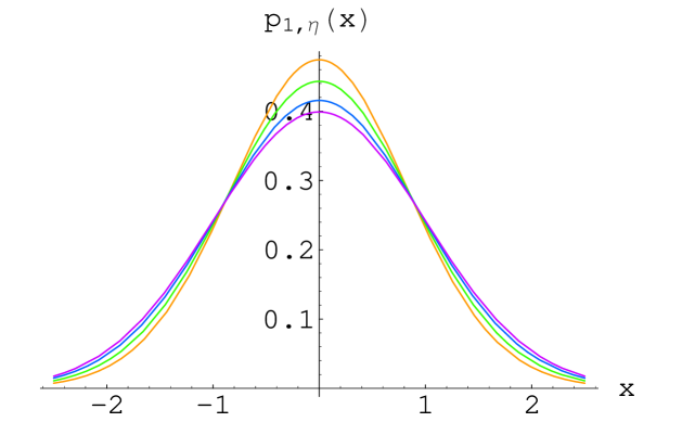
Figure 1: Plot of the marginal distribution $\mathbf{p}_{1,\eta}(x)$ for different values of $\eta$ [Orange $0.8$; Green $0.5$; Blue $0.2$]. The limiting Gaussian distribution $\eta=0$ is also plotted [Violet].

A careful asymptotic analysis (see Appendix A) of the convolution integral (3.1) gives for $x\rightarrow\pm\infty$:

$$\mathbf{p}_{1,\eta}(x)\approx\frac{1}{2\,\sqrt{2}\,\Gamma(3/2-\eta)}\,{\left(\frac{x}{2}\right)}^{-2\eta}\,e^{-x^{2}/2}$$ (30)

and for $\eta>0$ the decay is faster than Gaussian due to the power-law prefactor, in agreement with the plots in figure 1.

The other marginals can be computed as well:

$$\mathbf{p}_{2,\eta} (x,y)=\frac{e^{-\frac{(x+y)^{2}}{4}}}{4\sqrt{\pi}\Gamma\left(\frac{3}{2}-\eta\right)}\Gamma\left(1-\eta,\frac{(x-y)^{2}}{4}\right)$$ (31)

$$\mathbf{p}_{3,\eta} (x,y,t)=\frac{e^{-\frac{1}{2}(x^{2}+y^{2}+t^{2})}}{\pi^{3/2}2^{3-2\eta}\Gamma\left(\frac{3}{2}-\eta\right)}\times$$

$$\times\left\{\frac{a^{1/2-\eta}\sqrt{\pi/2}\Gamma(\eta-1/2)~{}_{1}F_{1}(1/2,3/2-\eta,a/4)}{\Gamma(\eta)}+\right.$$

$$+\left.2^{1/2-2\eta}\Gamma(1/2-\eta)~{}_{1}F_{1}(\eta,1/2+\eta,a/4)\right\}$$ (32)

where we defined $a=(x-y)^{2}+2t^{2}$ and ${}_{1}F_{1}(\hat{\alpha},\hat{\beta},z)$ is the Kummer confluent hypergeometric function.

At this stage, we make the following important remarks:

1. For $\eta\rightarrow 0$, it is straightforward to check that (31) and (32) reproduce the expected GUE factorized distributions:

   $$\mathbf{p}_{2,\eta=0}(x,y) =\frac{e^{-\frac{1}{2}(x^{2}+y^{2})}}{2\pi}$$ (33)

   $$\mathbf{p}_{3,\eta=0}(x,y,t) =\frac{e^{-\frac{1}{2}(x^{2}+y^{2}+t^{2})}}{(2\pi)^{3/2}}$$ (34)

2. For $\eta\rightarrow 1/2$ (a noticeable special case, see next subsection), all the marginal distributions remain well-defined. In particular, the apparent divergences of the Gamma functions in (32) cancel out and the final density reads:

   $$\mathbf{p}_{3,\eta=1/2}(x,y,t)=\frac{1}{\pi^{3/2}2^{5/2}}e^{a/8}K_{0}(a/8)$$ (35)

   where $K_{0}(x)$ is a Modified Bessel Function of degree 0 of the Second Kind.

3.2 Spectral properties.

As already discussed at the end of the previous subsection, the case $\eta=1/2$ is particularly interesting, as the jpd of eigenvalues (18) collapses onto the Gaussian Orthogonal Ensemble (GOE) one ($\beta_{\mathrm{eff}}=1$). The matrices belonging to GOE have independent and real entries and the orthogonal group as SG. Instead, $\eta$-UE reproduces the GOE spectral statistics while having complex and correlated entries and the unitary group as SG. This is a first example of a curious phenomenon, which we call spectral twinning (see Section 5.1) between ensembles having the same spectral properties (same jpd of eigenvalues) but different SG (different number of independent real variables). As a consequence, the connection between the exponent of the Vandermonde $\beta_{\mathrm{eff}}$ and the SG of the ensemble becomes much more blurred and potentially deceptive than for the classical $\beta=1,2,4$ ensembles.

In this section and in Appendix B, we compute for completeness the average spectral density for our $\eta$-UE model with Gaussian weight function, as this calculation does not appear to have been carried out explicitly before. The raw level spacing has already been computed in the context of a $2\times 2$ $\beta$-Hermite ensemble in lecaer .

The average spectral density $\rho_{\eta}(\lambda)$ and the gap probability $P_{\eta}(s)$ are given as usual by:

$$\rho_{\eta}(\lambda) =\int_{-\infty}^{\infty}P_{\eta}(\lambda,\lambda_{2})\,d\lambda_{2}$$ (36)

$$P_{\eta}(s) =\int_{-\infty}^{\infty}P_{\eta}(\lambda_{1},\lambda_{1}+s)d\lambda_{1}$$ (37)

where in (37) and hereafter, $s$ is meant as the raw spacing, without any unfolding procedure being performed on the spectrum.

They can be computed exactly from (18) as (see Appendix B):

$$\rho_{\eta}(\lambda) =\frac{e^{-\lambda^{2}}}{2^{3/2-\eta}\sqrt{\pi}}\,_{1}F_{1}(3/2-\eta,1/2,\lambda^{2}/2)$$ (38)

$$P_{\eta}(s) =2\sqrt{\pi}\mathrm{K}_{\eta}~{}s^{2-2\eta}e^{-s^{2}/4}$$ (39)

where $\mathrm{K}_{\eta}$ is defined in (19).

It is easy to check that (38) recovers for $\eta=0,1/2,1$ the expected spectral densities (GUE, GOE and purely Gaussian, respectively):

$$\rho_{0}(\lambda) =\frac{e^{-\lambda^{2}/2}(1+\lambda^{2})}{2\sqrt{2\pi}}$$ (40)

$$\rho_{1/2}(\lambda) =\frac{e^{-\lambda^{2}}(2+\sqrt{2\pi}e^{\lambda^{2}/2}\lambda~{}\mathrm{erf}(\lambda/\sqrt{2}))}{4\sqrt{\pi}}$$ (41)

$$\rho_{1}(\lambda) =\frac{e^{-\lambda^{2}/2}}{\sqrt{2\pi}}$$ (42)

where $\mathrm{erf}(z)=(2/\sqrt{\pi})\int_{0}^{z}e^{-t^{2}}dt$.

The results (38) and (39) are numerically checked by actual diagonalization of $\eta$-UE matrices in the next Section.

3.3 Numerical Simulations.

We report in this section the results for the spectral density and the level spacing, obtained by direct sampling of $\eta$-UE matrices.

The algorithm proceeds as follows: by rejection sampling NR we draw a random number $\bar{x}$ from the marginal distribution $\mathbf{p}_{1,\eta}(x)$ (3.1). Then, from the marginal distribution (31), we determine the conditional probability:

$$\mathbf{p}_{\eta}(y|\bar{x})=\frac{\mathbf{p}_{2,\eta}(\bar{x},y)}{\mathbf{p}_{1,\eta}(\bar{x})}$$ (43)

and again we draw a random number $\bar{y}$ from (43). This procedure is iterated through the higher order marginals up to identifying the four variables $(\bar{x},\bar{y},\bar{t},\bar{s})$ from which one sample of $\eta$-UE is constructed. Each sample is then diagonalized and we give a histogram of the eigenvalues and of the gaps between the two eigenvalues over a total number of $75000$ samples for each plot.

We include three plots for the spectral density (Fig. 2,3,4) ($\eta=0,0.45,0.75$ respectively) and three plots for the gap probability (Fig. 5,6,7 ) ($\eta=0,0.5,0.75$ respectively). On top of the histograms, we plot the theoretical results (38) and (39). The agreement is excellent.

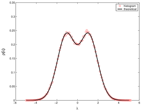
Figure 2: Plot of the average density of states $\rho_{\eta}(\lambda)$ for $\eta=0$

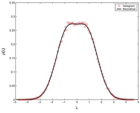
Figure 3: Plot of the average density of states $\rho_{\eta}(\lambda)$ for $\eta=0.45$

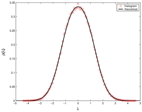
Figure 4: Plot of the average density of states $\rho_{\eta}(\lambda)$ for $\eta=0.75$. Beyond the value $\eta=0.5$, the density becomes unimodal.

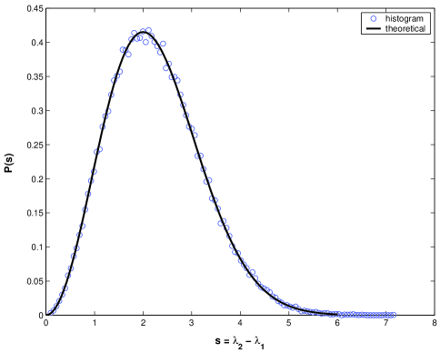
Figure 5: Plot of the gap probability $P_{\eta}(s)$ for $\eta=0$

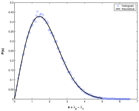
Figure 6: Plot of the gap probability $P_{\eta}(s)$ for $\eta=0.5$

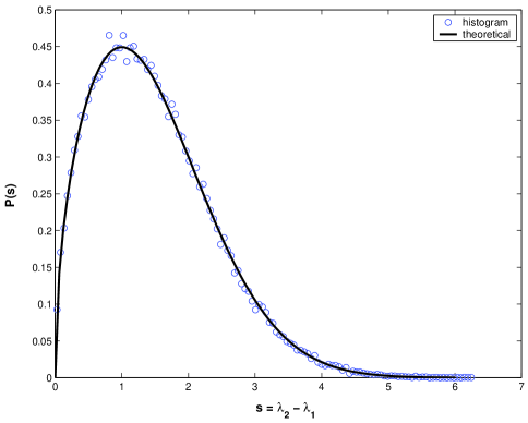
Figure 7: Plot of the gap probability $P_{\eta}(s)$ for $\eta=0.75$

4 Second Task: Non-Gaussian weight function.

In this section, we show how to devise a weight function depending on the parameter $\eta\in[1/2,1]$ such that the level spacing for the corresponding $\eta$-UE ensemble develops a Wigner-Poisson crossover. In principle, the solution we offer can be taken as a guideline for the general problem described in the Introduction as Task 2. Even though the two above cases (Poisson and Wigner) absorb the vast majority of literature on these issues, nevertheless few instances of ’non-standard’ gap distributions have been also reported kudo pineda jakub . Our hope is that the tool we propose here may be used to comprise even these fairly anomalous cases into the universal and otherwise very successful framework of RM theory.

The starting point is the general jpd of eigenvalues (10):

$$P_{\eta}^{(\mathcal{W})}(\lambda_{1},\lambda_{2})\propto\mathcal{W}^{\star}_{\eta}(\lambda_{1},\lambda_{2})|\lambda_{2}-\lambda_{1}|^{2-2\eta}$$ (44)

where the superscript $(\mathcal{W})$ recalls that the weight function is still to be determined.

The gap probability for a general weight function can be formally written as:

$$P_{\eta}^{(\mathcal{W})}( s)=\int_{-\infty}^{\infty}\int_{-\infty}^{\infty}~{}d\lambda_{1}d\lambda_{2}\mathcal{W}^{\star}_{\eta}(\lambda_{1},\lambda_{2})|\lambda_{2}-\lambda_{1}|^{2-2\eta}\times$$

$$\times\delta(\lambda_{2}-\lambda_{1}-s)=s^{2-2\eta}\int_{-\infty}^{\infty}\mathcal{W}^{\star}_{\eta}(\lambda_{1},\lambda_{1}+s)d\lambda_{1}$$ (45)

Apart from being symmetric in the eigenvalues , non-negative everywhere and normalizable, the sought $\mathcal{W}^{\star}_{\eta}(\lambda_{1},\lambda_{2})$ should satisfy the following constraints:

$$\int_{-\infty}^{\infty}\mathcal{W}^{\star}_{\eta=1}(x,x+s)dx \propto\exp(-|s|)$$ (46)

$$\int_{-\infty}^{\infty}\mathcal{W}^{\star}_{\eta=1/2}(x,x+s)dx \propto\exp(-\alpha s^{2})$$ (47)

where $\alpha$ is a numerical constant, in such a way that (4) reduces exactly to Poisson for $\eta=1$ or Wigner for $\eta=1/2$. Indeed, the Wigner distribution in (3) corresponds to the gap probability for a GOE ensemble of $2\times 2$ real matrices ($\beta_{\mathrm{eff}}=1$) and thus has to be realized in $\eta$-UE for $\eta=1/2$ and for a Gaussian weight function (47). The other limit is when there are no correlations among the eigenvalues ($\eta=1$) and thus one may expect a Poisson distribution for the level spacing (46).

Note that the prefactors in (46) and (47) can be restored at the end by normalization and in Eq. (46) we use the absolute value of $s$ since the function must be symmetric in $s$.

In order to find an appropriate weight function satisfying the given constraints, we first make the ansatz:

$$\mathcal{W}^{\star}_{\eta}(x,y)=\phi_{\eta}(x)\phi_{\eta}(y)$$ (48)

where $\phi_{\eta}(x)$ is an even function of $x$.

Now, from (46) one has the convolution:

$$\int_{-\infty}^{\infty}\phi_{1}(x)\phi_{1}(s-x)dx=\exp(-|s|)$$ (49)

which gives in Fourier space:

$$[\tilde{\phi}_{1}(k)]^{2}=\frac{2}{k^{2}+1}$$ (50)

Thus:

$$\tilde{\phi}_{1}(k)=\sqrt{\frac{2}{k^{2}+1}}$$ (51)

Inverting (51), we get:

$$\phi_{1}(x)=\frac{\sqrt{2}}{\pi}K_{0}(x)$$ (52)

where $K_{0}(x)$ is a Modified Bessel Function of degree $0$ of the Second Kind.

Similarly, for $\eta=1/2$ one gets:

$$\phi_{1/2}(x)=[4\alpha/\pi]^{1/4}e^{-2\alpha x^{2}}$$ (53)

In order to obtain the function interpolating between (52) and (53), we notice that $K_{0}(x)$ has the following integral representation GR :

$$K_{0}(x)=\frac{1}{2}\int_{0}^{\infty}dt\frac{e^{-\gamma t-x^{2}/(4\gamma t)}}{t}.$$ (54)

where $\gamma$ is any real and positive parameter.

Then one can write:

$$\phi_{1}(x)=\mathrm{B}_{1}\,\int_{0}^{\infty}\frac{dt}{t}\exp\left(-\gamma t-\frac{x^{2}}{4\gamma t}\right)$$ (55)

where $\mathrm{B}_{1}=1/(\pi\sqrt{2})$. On the other hand, $\phi_{1/2}(x)$ can also be written trivially in a similar integral representation as:

$$\phi_{1/2}(x)=\mathrm{B}_{1/2}\int_{0}^{\infty}\exp\left(-\bar{\gamma}t-x^{2}/{4\bar{\gamma}}\right)dt$$ (56)

where $\mathrm{B}_{1/2}=2^{-5/2}\alpha^{-3/4}{\pi}^{-1/4}$ and $\bar{\gamma}:=1/(8\alpha)$ . Thus, for general $1/2\leq\eta\leq 1$, a natural definition of $\phi_{\eta}(x)$ interpolating the two bordering cases would be:

$$\phi_{\eta}(x)=\mathrm{B}_{\eta}\int_{0}^{\infty}t^{1-2\eta}\exp\left(-\frac{t}{8\alpha}-\frac{2\alpha x^{2}}{t^{2\eta-1}}\right)\,dt.$$ (57)

The corresponding weight function $\mathcal{W}^{\star}_{\eta}(x,y)$ is given by the product in (48) and satisfies all the given constraints. We will refer to this weight function as a Generalized Bessel weight.

The reader may be puzzled by the non-standard expression (57) and may wonder whether the resulting weight function $\mathcal{W}^{\star}_{\eta}(\lambda_{1},\lambda_{2})$ is indeed expressible in terms of traces of powers of $\mathcal{X}$, a fact which is not obvious at first sight. Actually, this can be shown easily by expressing the individual eigenvalues as:

$$\lambda_{1,2}=\frac{s_{1}\pm\sqrt{2s_{2}-s_{1}^{2}}}{2}$$ (58)

where $s_{j}=\mathrm{Tr}\mathcal{X}^{j}$.

The gap probability can then be computed from (4). For arbitrary $\eta$, the integral in (4) is difficult to carry out for all $s$. However, the large $s$ tail of $P_{\eta}^{(\mathcal{W})}(s)$ can be easily derived by the saddle point method and has the following behavior:

$$P_{\eta}^{(\mathcal{W})}(s)\propto\exp\left[-\eta(2\eta-1)^{-1+1/{2\eta}}\,(2\alpha)^{-1+1/\eta}\,s^{1/\eta}\right].$$ (59)

One can check easily that it reduces to the known Wigner and Poisson cases for $\eta=1/2$ and $\eta=1$ respectively. Thus our ensemble smoothly interpolates the tail of the gap distribution between the two known cases, although the full behavior of $P_{\eta}^{(\mathcal{W})}(s)$ is different from any previous proposals (e.g. Brody and Berry-Robnik distributions).

Also the spectral density can be numerically investigated after some intermediate algebraic steps that we include in Appendix C for completeness. The resulting plots for different values of $\zeta:=2\eta-1$ ($0\leq\zeta\leq 1$) and $\alpha=1$ are reported in Fig. 8.

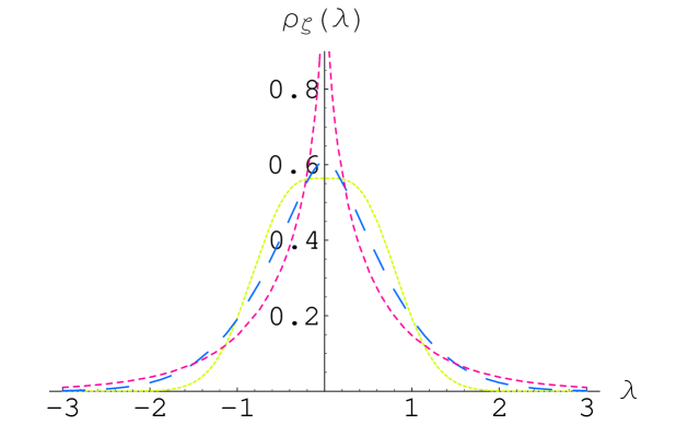
Figure 8: Plot of the spectral density $\rho_{\zeta}(\lambda)$ for the following different values of $\zeta$: 0 (dotted green), 0.45 (long-dashed blue), 0.9 (short-dashed magenta). Note the pure GOE density for $\zeta=0$ and the peculiar trend towards an integrable divergence at the origin as $\zeta\rightarrow 1^{-}$.

In summary, the Generalized Bessel weight function $\mathcal{W}^{\star}_{\eta}(\lambda_{1},\lambda_{2})=\phi_{\eta}(\lambda_{1})\phi_{\eta}(\lambda_{2})$, where $\phi_{\eta}(x)$ is given by (57) and $\lambda_{1,2}$ are expressed in terms of traces as (58) generates a $\eta$-UE model having:

• rotational invariance;

• $0\leq\beta_{\mathrm{eff}}\leq 1$;

• prescribed level spacing (interpolating between Poisson and Wigner);

• a novel transitional profile for the spectral density as documented in Fig. 8.

and is to be regarded as complementary to the model proposed in chau . Note also that the above results are still valid in the range $[0,1/2]$ for $\eta$, corresponding to a GUE-Poisson crossover.

5 Generalizations.

The work presented here can be extended in several directions. We would like to offer a list of issues that can be tackled in future researches.

5.1 Different Dyson class $\beta$.

We confined our investigation to hermitian matrices $(\beta=2)$, since the identity (9) involves exactly the exponent $2$ for the Vandermonde, but it is not harmful to consider the following obvious relations instead:

$$|\lambda_{2}-\lambda_{1}| =\sqrt{2\mathrm{Tr}\mathcal{X}^{2}-(\mathrm{Tr}\mathcal{X})^{2}}$$ (60)

$$|\lambda_{2}-\lambda_{1}|^{4} =\left[2\mathrm{Tr}\mathcal{X}^{2}-(\mathrm{Tr}\mathcal{X})^{2}\right]^{2}$$ (61)

and reformulate the model for real symmetric and quaternion self-dual Hermitian matrices respectively:

$$\mathcal{X}_{\mathbb{R}}=\begin{pmatrix}x&t\\ t&y\\ \end{pmatrix}\qquad\mathcal{X}_{\mathbb{H}}=\left(\begin{array}[]{cc|cc}x&0&t+is&u+iv\\ 0&x&-u+iv&t-is\\ \hline\cr t-is&-u-iv&y&0\\ u-iv&t+is&0&y\end{array}\right)$$ (62)

having respectively $3$ and $6$ real independent variables.

Example: real symmetric matrices with Gaussian weight function. In this case, the jpd of eigenvalues reads:

$$P_{\hat{\eta}}(\lambda_{1},\lambda_{2})\propto\exp\left(-\frac{1}{2}(\lambda_{1}^{2}+\lambda_{2}^{2})\right)|\lambda_{2}-\lambda_{1}|^{1-\hat{\eta}}$$ (63)

where we rename the running parameter as $0\leq\hat{\eta}\leq 1$, and the jpd of entries is given by:

$$\mathbf{P}_{\hat{\eta}}^{\star}=\mathrm{C}_{\hat{\eta}}\frac{e^{-\frac{1}{2}\mathrm{Tr}\mathcal{X}_{\mathbb{R}}^{2}}}{[2\mathrm{Tr}\mathcal{X}_{\mathbb{R}}^{2}-(\mathrm{Tr}\mathcal{X}_{\mathbb{R}})^{2}]^{\hat{\eta}/2}}$$ (64)

The expression (63), when compared with the corresponding one for hermitian matrices (18), leads immediately to the following observation: if the parameter $\eta$ is chosen in $[1/2,1]$ and $\hat{\eta}:=2\eta-1$, then the two ensembles (real and complex) get twinned, i.e. they share the same spectral properties, despite belonging to different classes of invariance and having even a different number of independent variables. This spectral twinning is a curious byproduct of our construction, which was already remarked in subsection 3.2. While it is premature to imagine possible physical application for this, nonetheless we believe that this peculiar property, which does not hold for any classical invariant ensemble and of course neither for the $\beta$-ensembles, deserves further investigations and may be related to some group-theoretical features of $\eta$-XE (X=O,U,S) yet undiscovered. Note also that this property would survive even for $N\times N$ $\eta$-XE and holds for any acceptable weight function.

5.2 Different classical weights.

A whole group of novel $2\times 2$ ensembles can be generated by choosing different weight functions among the classical ones, as:

1. Laguerre and Jacobi (to make contact with DE );

2. fixed and restricted trace ensembles rosen akemann lecaer2 ;

3. quartic and higher order potentials Brezin ;

4. power laws bertuola toscano abulmagd ;

In view of subsection 5.1, all the above can be generated starting from real, complex and quaternion entries and a number of twinnings can be found. In particular, the $\beta$-version of (3) and (4) has not been constructed as an actual random matrix ensemble so far, while this problem can be tackled using the method we presented here.

5.3 Extended range for $\eta$.

Provided that the weight function decays fast enough at infinity in order to ensure convergence of the integrals involved, it is possible to extend considerably the range of variability for $\eta$ in the two examples above as well as in any future study. Taken the Gaussian case as an example (Section 3), the following extensions can be considered:

• $\eta<0$: a negative $\eta$ in (18) enhances (instead of suppressing) the correlations among eigenvalues and extends the range of variability for the effective Dyson index from $[0,2]$ to $[0,+\infty)$.

• $1<\eta<3/2$: this case is even more interesting as it allows to generate an Anti-$\eta$-UE ensemble whose jpd of eigenvalues would be given by:

  $$P(\lambda_{1},\lambda_{2}):=\tilde{\mathrm{K}}_{\eta}\exp\left(-\frac{1}{2}(\lambda_{1}^{2}+\lambda_{2}^{2})\right)|\lambda_{2}-\lambda_{1}|^{-\beta_{\mathrm{eff}}}\qquad 0<\beta_{\mathrm{eff}}<1$$ (65)

  i.e. with a negative Dyson index. The most immediate consequence is that the peculiar level repulsion has to be replaced by a fairly uncommon (at least in RM studies) level attraction. The tendency of energy levels to cluster instead of repelling apart has been found in several disordered many-body systems hsu2 jalab skv bolte but has not received equal attention in the context of invariant RM. The Anti-$\eta$-UE is likely to lead to a ’non-Wigner’-surmise for the level spacing to be compared with the studies cited above. We offer this idea as our last contribution in this paper.

6 Conclusions.

Before summarizing the main results of this paper, we propose the synthetic Table II, containing the most relevant features of the ensembles considered in this work.

Name	Weight	Inv.	Indep.	Entries	Size	$\beta_{\mathrm{eff}}$
$\beta$-Hermite	Gaussian	N	Y	$\mathbb{R}$	$N\geq 2$	$>0$
GUE	Gaussian	Y	Y	$\mathbb{C}$	$N\geq 2$	$2$
GOE	Gaussian	Y	Y	$\mathbb{R}$	$N\geq 2$	$1$
$\eta$-UE	Gaussian	Y	N	$\mathbb{C}$	$N=2$	$[0,2]$
	Generalized Bessel	Y	N	$\mathbb{C}$	$N=2$	$[0,1]$
Anti-$\eta$-UE	Gaussian	Y	N	$\mathbb{C}$	$N=2$	$[-1,0]$
$\beta$-XE	Arbitrary	Y	N	$\mathbb{R},\mathbb{C},\mathbb{H}$	$N=2$	Arbitrary

Table 2: Columnwise: Name of the ensemble, Classical weight or weight function, Rotational Invariance, Independent Entries, Type of Entries, Size of the matrices, Range for $\beta_{\mathrm{eff}}$ (exponent of the Vandermonde). In the last row, different combinations of symmetry class, weight function and range for $\eta$ may be exploited according to Section 5.

The main results of the paper can be summarized as follows:

1. Although the $\beta$-index of an invariant ensemble is determined uniquely by its symmetry group, through a rather unusual expansion of the Vandermonde-squared on the basis of power sums it is possible to neutralize (entirely or partially) the coupling between the eigenvalues introducing suitable correlations among the entries. Hence, one has to be careful in deducing the SG of the ensemble from the exponent of the Vandermonde coupling $\beta_{\mathrm{eff}}$, as this connection may be deceptive.

2. Using this tool, we have constructed an invariant $2\times 2$ version of the $\beta$-ensembles of Dumitriu and Edelman. This matrix model is completely defined assigning a Symmetry Group (Orthogonal, Unitary, Symplectic), a weight function and a certain range for $\eta$:

   • For the Unitary case, with Gaussian weight function and $0\leq\eta\leq 1$, both the marginal distribution of the entries and the spectral properties have been computed analytically and have been tested by numerical sampling of $\eta$-UE matrices. The case $\beta_{\mathrm{eff}}=0$, corresponding to independent normally distributed eigenvalues, is particularly interesting and can be obtained for $\eta=1$.

   • For the Unitary case, with a Generalized Bessel weight function and $1/2\leq\eta\leq 1$, we generate $\eta$-UE matrices with a level spacing profile interpolating between Poisson and Wigner. Both analytical and numerical results have been provided.

3. Unlike the classical invariant ensembles, our ensembles belonging to different symmetry classes may display the same spectral properties for a suitable range of the free parameter. We called this curious phenomenon spectral twinning and we leave a deeper understanding of it as an open problem.

4. An extended range for $\eta$ may lead to invariant ensembles whose eigenvalues tend to cluster instead of repelling apart due to a negative Dyson index $\beta$. We are not aware of any previous proposal in this direction, even though this behavior is fairly common in the study of disordered many-body systems.

While generalizations to bigger sizes $N>2$ appear difficult to be tackled analytically, nonetheless the model we presented here displays non-trivial and often surprising features, which make us hope that the proposed technical tool may prove useful in future RM studies.

Appendix A Asymptotic Analysis of $\mathbf{p}_{1,\eta}(x)$.

We start from the exact expression of the marginal distribution (3.1):

$$\mathbf{p}_{1,\eta}(x)=\frac{1}{2\sqrt{\pi}\Gamma(3/2-\eta)}\,\int_{-\infty}^{\infty}dy\Gamma(1-\eta,y^{2})\,e^{-(x+y)^{2}}$$ (66)

We first divide the integral into 2 parts: over $[-\infty,0]$ and $[0,\infty]$. In the first part, we also make a change of variable $y\to-y$. This gives:

$$\mathbf{p}_{1,\eta}(x) =\frac{1}{2\sqrt{\pi}\Gamma(3/2-\eta)}\,\left[\int_{0}^{\infty}dy\Gamma(1-\eta,y^{2})\,e^{-(x-y)^{2}}+\right.$$

$$\left.+\int_{0}^{\infty}dy\Gamma(1-\eta,y^{2})e^{-(x+y)^{2}}\right]=$$

$$=\frac{1}{2\sqrt{\pi}\Gamma(3/2-\eta)}\left[J_{1}(x)+J_{2}(x)\right]$$ (67)

Consider first $J_{1}(x)$. Clearly, the most important contribution to the integral comes from the region around $y=x$ for large $x$. Since $y$ is large in this regime, we can replace $\Gamma(1-\eta,y^{2})$ by its leading asymptotic form:

$$\Gamma(1-\eta,y^{2})\approx e^{-y^{2}}\,y^{-2\eta}.$$ (68)

Substituting this in the expression for $J_{1}(x)$ we get, to leading order:

$$J_{1}(x)\approx\int_{\bar{a}}^{\infty}dy\,e^{-y^{2}}\,y^{-2\eta}\,e^{-(x-y)^{2}}$$ (69)

where the lower limit $\bar{a}\sim O(1)$. Rewriting the exponential we get:

$$J_{1}(x)\approx e^{-x^{2}/2}\int_{\bar{a}}^{\infty}\,dy\,y^{-2\eta}\,e^{-2(y-x/2)^{2}}$$ (70)

Making a change of variable, $\sqrt{2}\,(y-x/2)=u$, we get for large $x$:

$$J_{1}(x)\approx\frac{1}{\sqrt{2}}\,e^{-x^{2}/2}\,(x/2)^{-2\eta}\,\int_{\sqrt{2}(\bar{a}-x/2)}^{\infty}du\,e^{-u^{2}}$$ (71)

In the $x\to\infty$ limit, the lower limit of the integral can be replaced by $-\infty$. This finally gives:

$$J_{1}(x)\approx\sqrt{\frac{\pi}{2}}\,e^{-x^{2}/2}\,(x/2)^{-2\eta}$$ (72)

Now for the integral $J_{2}(x)$, for large $x$, the most important contribution comes from the region $y=0$. Thus, it is easy to see that for large $x$, $J_{2}(x)\approx e^{-x^{2}}\int_{0}^{\infty}dy\Gamma(1-\eta,y^{2})=b_{\eta}e^{-x^{2}}$ where $b_{\eta}$ is a constant. Thus, clearly $J_{2}(x)$ decays faster than $J_{1}(x)$ and hence can be neglected for large $x$.

Thus, for large $x$, to leading order we get:

$$\mathbf{p}_{1,\eta}(x)\approx\frac{1}{2\,\sqrt{2}\,\Gamma(3/2-\eta)}\,{\left(\frac{x}{2}\right)}^{-2\eta}\,e^{-x^{2}/2}$$ (73)

It is easy to check that for $\eta=0$, (73) reduces to the standard Gaussian.

Appendix B Spectral Density for the Gaussian weight function.

Consider the joint distribution of the two eigenvalues (18):

$$P_{\eta}(\lambda_{1},\lambda_{2})=\mathrm{K}_{\eta}\,e^{-(\lambda_{1}^{2}+\lambda_{2}^{2})/2}\,|\lambda_{2}-\lambda_{1}|^{2-2\eta}$$ (74)

where the normalization constant $\mathrm{K}_{\eta}$ is given by (19).

We want to compute the average density of states which is precisely the marginal distribution:

$$\rho_{\eta}(\lambda)=\int_{-\infty}^{\infty}P_{\eta}(\lambda,\lambda_{2})\,d\lambda_{2}$$ (75)

Substituting the jpd from (74) into (75) and making a change of variable $\lambda_{2}-\lambda=x$ we get:

$$\rho_{\eta}(\lambda)=\mathrm{K}_{\eta}\,e^{-\lambda^{2}/2}\,\int_{-\infty}^{\infty}e^{-(\lambda+x)^{2}/2}\,|x|^{2-2\eta}\,dx$$ (76)

Divide the integral into two parts: over $[-\infty,0]$ and $[0,\infty]$ and write it as:

$$\rho_{\eta}(\lambda) =\mathrm{K}_{\eta}\,e^{-\lambda^{2}/2}\,\left[\int_{0}^{\infty}\left\{e^{-(\lambda-x)^{2}/2}+e^{-(\lambda+x)^{2}/2}\right\}\times\right.$$

$$\left.\times\,x^{2-2\eta}\,dx\right]=\mathrm{K}_{\eta}\,e^{-\lambda^{2}/2}\,\left[I_{1}(\lambda)+I_{2}(\lambda)\right]$$ (77)

The first integral can be rewritten as:

$$I_{1}(\lambda) =e^{-\lambda^{2}}\,\int_{0}^{\infty}\,e^{x\lambda-x^{2}/2}\,x^{2-2\eta}\,dx=e^{-\lambda^{2}/4}\,\Gamma(3-2\eta)\,\times$$

$$\times D_{2\eta-3}(-\lambda)$$ (78)

where $D_{p}(z)$ is the parabolic cylinder function of index $p$ and argument $z$ GR . Similarly $I_{2}(\lambda)=I_{1}(-\lambda)$. Adding the two we get:

$$\rho_{\eta}(\lambda)=\mathrm{K}_{\eta}\,\Gamma(3-2\eta)\,e^{-3\lambda^{2}/4}\,\left[D_{2\eta-3}(\lambda)+D_{2\eta-3}(-\lambda)\right]$$ (79)

We next use the identity (9.240) of GR :

$$D_{p}(z)+D_{p}(-z)=\frac{2^{p/2+1}\sqrt{\pi}e^{-z^{2}/4}}{\Gamma((1-p)/2)}\,\,_{1}F_{1}(-p/2,1/2,z^{2}/2)$$ (80)

where ${}_{1}F_{1}(\hat{\alpha},\hat{\beta},z)$ is the Kummer confluent hypergeometric function defined by the series:

$${}_{1}F_{1}(\hat{\alpha},\hat{\beta},z)=1+\frac{\hat{\alpha}}{\hat{\beta}}\frac{z}{1!}+\frac{\hat{\alpha}(\hat{\alpha}+1)}{\hat{\beta}(\hat{\beta}+1)}\frac{z^{2}}{2!}+\ldots$$ (81)

Using this identity in (79) we get:

$$\rho_{\eta}(\lambda) =\frac{\mathrm{K}_{\eta}\,2^{\eta-1/2}\,\sqrt{\pi}\,\Gamma(3-2\eta)}{\Gamma(2-\eta)}\,e^{-\lambda^{2}}\,\times$$

$$\times~{}_{1}F_{1}(3/2-\eta,1/2,\lambda^{2}/2)$$ (82)

We then use the explicit expression of $\mathrm{K}_{\eta}$ from (19) to get:

$$\rho_{\eta}(\lambda)=\,\frac{2^{3\eta-7/2}\Gamma(3-2\eta)}{\Gamma(3/2-\eta)\Gamma(2-\eta)}\,e^{-\lambda^{2}}\,_{1}F_{1}(3/2-\eta,1/2,\lambda^{2}/2)$$ (83)

We can further simplify the constant term by using the Gamma function identity (doubling formula):

$$\Gamma(2z)=\frac{2^{2z-1}}{\sqrt{\pi}}\,\Gamma(z)\,\Gamma(z+1/2)$$ (84)

This then gives our final formula:

$$\rho_{\eta}(\lambda)=\frac{e^{-\lambda^{2}}}{2^{3/2-\eta}\sqrt{\pi}}\,_{1}F_{1}(3/2-\eta,1/2,\lambda^{2}/2)$$ (85)

Appendix C Spectral Density for the Generalized Bessel weight function.

The spectral density for the Generalized Bessel weight function (48) is given by:

$$\rho_{\zeta}(\lambda)\propto\phi_{\zeta}(\lambda)\int_{-\infty}^{\infty}dy~{}\phi_{\zeta}(y)|\lambda-y|^{1-\zeta}$$ (86)

where the proportionality constant is just given by the normalization condition and we have slightly changed the notation $\phi_{\eta}(x)\rightarrow\phi_{\zeta}(x)$, where:

$$\phi_{\zeta}(x):=\int_{0}^{\infty}dt~{}t^{-\zeta}\exp\left(-\frac{t}{8\alpha}-2\alpha x^{2}t^{-\zeta}\right)$$ (87)

and $0\leq\zeta\leq 1$.

We aim to rewrite (86) in a form suitable for a numerical implementation, so from now on we will drop all the constant in front and we will normalize the numerical density to $1$ at the very end.

First, we define:

$$F_{\zeta}(x):=\int_{0}^{\infty}ds~{}s^{1-\zeta}\phi_{\zeta}(s+x)$$ (88)

and it is easy to check that:

$$\rho_{\zeta}(\lambda)\propto\phi_{\zeta}(\lambda)\left[F_{\zeta}(\lambda)+F_{\zeta}(-\lambda)\right]$$ (89)

Exploiting (87) and changing the order of integration, $F_{\zeta}(x)$ can be rewritten as:

$$F_{\zeta}(x)\propto\int_{0}^{\infty}dt~{}t^{-\zeta}\exp\left(-\frac{t}{8\alpha}-2\alpha x^{2}t^{-\zeta}\right)\int_{0}^{\infty}ds~{}s^{1-\zeta}\exp\left(-\varpi s^{2}-\kappa s\right)$$ (90)

where $\varpi:=2\alpha t^{-\zeta}$ and $\kappa:=4\alpha xt^{-\zeta}$.

The $s$-integral can be carried out analytically and thanks again to the identity (9.240) of GR we get:

$$F_{\zeta}(\lambda)+F_{\zeta}(-\lambda)\propto \int_{0}^{\infty}dt~{}t^{-\zeta^{2}/2}\exp\left(-\frac{t}{8\alpha}-2\alpha\lambda^{2}t^{-\zeta}\right)\times$$

$$\times~{}_{1}F_{1}\left(1-\zeta/2,1/2,2\alpha\lambda^{2}t^{-\zeta}\right)$$ (91)

Hence, the spectral density (89) is determined as the product of two integrals that are easily evaluated numerically. The results for different values of $\zeta$ and $\alpha=1$ are plotted in Fig. 8.

References

- (1) E.P. Wigner, Proc. Cambridge Philos. Soc. 47, 790 (1951).
- (2) F.J. Dyson, J. Math. Phys. 3, 140 (1962).
- (3) M.L. Mehta, Random Matrices, Elsevier-Academic Press, 3rd Edition (2004).
- (4) E. Caurier, B. Grammaticos and A. Ramani, J. Phys. A: Math. Gen. 23, 4903 (1990).
- (5) G. Lenz and F. Haake, Phys. Rev. Lett. 67, 1 (1991).
- (6) P. Chau Huu-Tai, N.A. Smirnova and P. Van Isacker, J. Phys. A: Math. Gen. 35, L199 (2002).
- (7) Z. Ahmed and S.R. Jain, J. Phys. A: Math. Gen. 36, 3349 (2003).
- (8) M. Araujo, E. Medina and E. Aponte, Phys. Rev. E 60, 3580 (1999).
- (9) V.K.B. Kota and S. Sumedha, Phys. Rev. E 60, 3405 (1999).
- (10) Z. Ahmed, Phys. Lett. A 308, 140 (2003).
- (11) A.D. Jackson, B. Lautrup, P. Johansen and M. Nielsen, Phys. Rev. E 66, 066124 (2002).
- (12) S.N. Evangelou and A.Z. Wang, Phys. Rev. B 47, 13126 (1993).
- (13) A.S. Sabbah, Il Nuovo Cimento B 114, 1131 (1999).
- (14) N. Ullah, Indian Journal of Physics B 70B(3), 253 (1996).
- (15) Y. Alhassid and R.D. Levine, Phys. Rev. Lett. 57, 2879 (1986).
- (16) J. Shaffaf, Adv. Studies Theor. Phys. 1, 39 (2007).
- (17) W. Van Assche, J. Appl. Prob. 23, 1019 (1986).
- (18) I. Dumitriu and A. Edelman, J. Math. Phys. 43, 5830 (2002).
- (19) O. Bohigas, in Chaos and Quantum Physics, Proceedings of the Les Houches Summer School, Session L11, (1989), edited by M.-J. Giannoni, A. Voros and J. Zinn-Justin (Elsevier, New York, 1991).
- (20) P. Vivo, S.N. Majumdar and O. Bohigas, J. Phys. A: Math. Theor. 40(16), 4317 (2007).
- (21) I. Dumitriu and A. Edelman, J. Math. Phys. 47, 063302 (2006).
- (22) P.J. Forrester and E.M. Rains, Probability Theory and Related Fields 131(1), 1 (2005).
- (23) R. Killip and I. Nenciu, International Mathematics Research Notices (50), 2665 (2004).
- (24) R.A. Lippert, J. Math. Phys. 44, 4807 (2003).
- (25) A. Edelman and B.D. Sutton, Foundations of Computational Mathematics, OF1 (2007).
- (26) K. Życzkowski and M. Kuś, Phys. Rev. E 53, 319 (1996).
- (27) T. Baker and P. Forrester, Commun. Math. Phys. 188, 175 (1997).
- (28) O. Bohigas and J. Flores, Phys. Lett. B 34, 261 (1971).
- (29) J.B. French and S.S.M. Wong, Phys. Lett. B 33, 449 (1970).
- (30) T. Guhr, A. Müller-Groeling and H.A. Weidenmuller, Physics Reports 299(4), 189-425 (1998).
- (31) T.A. Brody, Lett. Nuovo Cimento 7, 482 (1973).
- (32) M.V. Berry and M. Robnik, J. Phys. A: Math. Gen. 17, 2413 (1984).
- (33) T. Cheon, Phys. Rev. Lett. 65(5), 529 (1990).
- (34) N. Ullah, Phys. Rev. E 57(1), 350 (1998).
- (35) M.S. Hussein and M.P. Pato, Phys. Rev. Lett. 70(8), 1089 (1993).
- (36) G.V. Dunne, Int. Journ. Mod. Phys. B 7(28), 4783 (1993).
- (37) I.G. Macdonald, Symmetric functions and Hall polynomials, Oxford Mathematical Monographs. The Clarendon Press, Oxford University Press, New York (1979).
- (38) D.J.E. Callaway, Phys. Rev. B 43, 8641 (1991).
- (39) I.S. Gradshteyn and I.M. Ryzhik, Table of Integrals, Series, and Products, ed. Alan Jeffrey and Daniel Zwillinger, 7th edition (2007).
- (40) G. Le Caër, C. Male and R. Delannay, Physica A 383, 190 (2007).
- (41) W.H. Press, S.A. Teukolsky, W.T. Vetterling and B.P. Flannery, Numerical Recipes: The Art of Scientific Computing, Cambridge University Press, 3rd edition (2007).
- (42) K. Kudo and T. Deguchi, Phys. Rev. B 68, 052510 (2003).
- (43) C. Pineda and T. Prosen, Phys. Rev. E 76, 061127 (2007).
- (44) J. Zakrzewski, K. Dupret and D. Delande, Phys. Rev. Lett. 74, 522 (1995).
- (45) N. Rosenzweig, in Statistical Physics, Brandeis Summer Institute (1962), edited by G. Uhlenbeck et al. (Benjamin, New York, 1963); B.V. Bronk, thesis, Princeton University, (1964), as quoted by Mehta .
- (46) G. Akemann, G.M. Cicuta, L. Molinari and G. Vernizzi, Phys. Rev. E 59, 1489 (1999).
- (47) G. Le Caër and R. Delannay, J. Phys. A: Math. Theor. 40, 1561 (2007).
- (48) E. Brézin and A. Zee, Nucl. Phys. B 402, 613 (1993).
- (49) A.C. Bertuola, O. Bohigas and M.P. Pato, Phys. Rev. E 70, 065102(R) (2004).
- (50) F. Toscano, R.O. Vallejos and C. Tsallis, Phys. Rev. E 69, 066131 (2004).
- (51) A.Y. Abul-Magd, Phys. Rev. E 71, 066207 (2005).
- (52) T.C. Hsu and J.C. Anglès d’Auriac, Phys. Rev. B 47, 14291 (1993).
- (53) R.A. Jalabert, J.-L. Pichard and C.W.J. Beenakker, Europhys. Lett. 24(l), 1 (1993).
- (54) M.A. Skvortsov and P.M. Ostrovsky, JETP Lett. 85, 72 (2007).
- (55) J. Bolte, G. Steil and F. Steiner, Phys. Rev. Lett. 69, 2188 (1992).