Active Galactic Nuclei with Double-Peaked Balmer Lines: I. Black Hole Masses and the Eddington ratios

Abstract

Using the stellar population synthesis, we model the stellar contribution for a sample of 110 double-peaked broad-lines AGNs from the Sloan Digital Sky Survey (SDSS). The stellar velocity dispersions ($\sigma_{*}$) are obtained for 52 double-peaked AGNs with obvious stellar absorption features, ranging from 106 to 284 km s^-1 . We also use multi-component profiles to fit $[\rm O~{}\sc{III}]$$\lambda\lambda 4959,5007$ and H$\beta$ emission lines. Using the well-established $M_{\rm bh}-\sigma_{*}$ relation, the black hole masses are calculated to range from $1.0\times 10^{7}$ to $5.5\times 10^{8}$ $M_{\odot}$, and the Eddington ratio from about 0.01 to about 1. Comparing with the known $R_{\rm BLR}-L$ relation, we can get the factor $f$, which indicates BLRs’ geometry, inclination and kinematics. We find that $f$ far deviates from 0.75, suggesting the non-virial dynamics of broad line regions. The peak separation is mildly correlated with the Eddington ratio and SMBH mass with almost the same correlation coefficients. It implies that it is difficult to detect obvious double-peak AGNs with higher Eddington ratios. Using the monochromatic luminosity at 5100Å to trace the bolometric luminosity, we find that the external illumination of the accretion disk is needed to produce the observed strength of H$\alpha$ emission line.

1. INTRODUCTION

Double-peaked broad Balmer emission profiles have been detected in about 200 active galactic nuclei (AGNs) (Eracleous & Halpern 1994, 2003; Strateva et al. 2003, 2006). A systematic survey of 110 sources (mostly broad-line radio loud AGNs at $z<0.4$) by Eracleous & Halpern (1994, 2003) suggested that about 20% sources show double-peaked broad Balmer lines. They found some characteristics of double-peaked AGNs: large full width at half maximum (FWHM) of H$\alpha$ line, ranging from about 4000 km s^-1  up to 40000 km s^-1 (e.g. Wang et al. 2005); about 50% starlight contribution in optical continuum around H$\alpha$; large equivalent widths of low-ionization forbidden lines; large [O I]/$[\rm O~{}\sc{III}]$ ratios. Strateva et al. (2003) found about 3% of the $z<0.332$ AGNs in the Sloan Digital Sky Survey (SDSS) are double-peaked AGNs, the fraction is smaller than that in radio-loud AGNs sample. Double-peaked lines have also been detected in some low-ionization nuclear emission line regions (LINERs), e.g. NGC1097, M81, NGC4450, NGC4203, NGC4579 (Storchi-Bergmann et al. 1993; Bower et al. 1996; Shields et al. 2000; Ho et al. 2000; Barth et al. 2001). It remains a matter as debate of the origin of the double-peaked profiles.

There are mainly three models to interpret the origin of the double-peaked profiles: the accretion disk (Chen & Halpern 1989; Eracleous & Halpern 1994, 2003; Gezari et al. 2007); the biconical outflow (Zheng et al. 1991; Abajas et al. 2006), and an anisotropic illuminated BLRs (Goad & Wanders 1996). More recently, observational test and physical consideration preferentially suggested that double-peaked profiles originate from the accretion disk within a radius from a few hundreds $R_{g}$ to about thousands $R_{g}$ ($R_{g}=GM_{\rm bh}/c^{2}$, $M_{\rm bh}$ is the SMBH mass) (Eracleous & Halpern 1994, 2003; Eracleous et al. 1997; Strateva et al. 2003, 2006; Gezari, et al. 2007). In order to interpret the sparsity of double-peaked AGNs, the origin of the single-peaked lines from accretion disk have been discussed (Eracleous & Halpern 2003 and the references therein): larger out radius of the line-emitting accretion disk; face-on accretion disk; and the accretion disk wind. Very few of the double-peaked high-ionization line profiles (e.g. CIV) is due to that these high ionization lines are thought to arise in a wind, not in the disk.

The masses of central supermassive black holes (SMBHs) can provide an important tool to understand the physics of double-peaked AGNs if we reliably estimate them (e.g. Lewis & Eracleous 2006; Lewis 2006). During the last decade, there is a striking progress on the study of central supermassive black holes. The stellar and/or gaseous dynamics is used to derive the SMBHs masses in nearby inactive galaxies. However, for AGNs, this method is very difficult because nuclei outshine their hosts. Fortunately, we can use the broad emission lines from BLRs (e.g. H$\beta$, H$\alpha$, Mg $\rm\sc II$, C$\rm\sc IV$) to estimate SMBH masses in AGNs by the reverberation mapping method and the empirical size-luminosity relation (Kaspi et al. 2000,2005; Vestergaard 2002; McLure & Jarvis 2002; Wu et al. 2004; Greene & Ho 2006a). There is a scaling factor with larger uncertainty, which is due to the unknown geometry and dynamics of broad line regions, BLRs (e.g. Krolik 2001; Collin et al. 2006). Nearby galaxies and AGNs seem to follow the same tight $M_{\rm bh}-\sigma_{*}$ relation, where $\sigma_{*}$ is the bulge velocity dispersion at eighth of the effective radius of the galaxy (Nelson et al. 2001; Tremaine et al. 2002; Greene & Ho 2006a, 2006b), although it remains controversial for narrow-line Seyfert 1 galaxies (NLS1s) (Mathur et al. 2001; Bian & Zhao 2004; Grupe & Mathur 2004; Watson et al. 2007). Lewis & Eracleous (2006) derived the black hole masses from $\sigma_{*}$ through fitting absorption lines of the Ca II triplet ($\lambda\lambda 8498,8542,8662$) for 5 double-peaked AGNs. Therefore the determination of the black hole mass from independent method of reverberation mapping is an useful prober to explore mysteries of the double peaked AGNs.

Significant stellar contribution in double-peaked AGNs makes the measurement of $\sigma_{*}$ possible and reliable. Here we present our results on the $\sigma_{*}$ measurements for the sample of 110 double-peaked AGNs from the Sloan Digital Sky Survey (SDSS) (Strateva et al. 2003). In section 2, we introduce our working sample selected from Strateva et al. (2003). Section 3 is data analysis. We present the calculations of the SMBH mass and the Eddington ratio, and discuss their errors in Section 4. Section 5 is contributed to the discuss of the BLRs in double-peaked AGNs. Section 6 is the relation between the peak separation and Mass/Eddington ratio. Section 7 is the Energy budget for double-peaked AGNs. Our conclusion is given in Section 8. The last section is our conclusion. All of the cosmological calculations in this paper assume $H_{0}=71\rm{~{}km~{}s^{-1}~{}Mpc^{-1}}$, $\Omega_{M}=0.27$, and $\Omega_{\Lambda}=0.73$.

2. Sample

Strateva et al. (2003) presented a sample of double-peaked AGNs ($z<0.332$) selected from SDSS. They used two steps to select candidates: (1) they selected the unusual ones from the symmetric lines using the spectral principal component analysis (PCA) (Hao et al. 2003); and (2) they fitted the H$\alpha$ region with a combination of several Gaussians, and only selected AGNs better fitted by two Gaussians. From the profiles of the broad components, several fitting parameters including the positions of the red and blue peaks ($\lambda_{\rm red}$, $\lambda_{\rm blue}$), the corresponding peak heights ($H_{\rm red}$, $H_{\rm blue}$), FWHMs were given in their Table 3. They investigated the multi-wavelength properties of these double-peaked AGNs and suggested that Eddington ratios could be large in these SDSS double-peaked AGNs (Strateva et al. 2006).

SDSS spectra cover the wavelength range of 3800-9200 Å with a spectral resolution of $1800<R<2100$. The fiber diameter in the SDSS spectroscopic survey is 3” on the sky. At the mean redshift of 0.24 in the sample of Strateva et al. (2003), the projected fiber aperture diameter is 13.2 kpc, typically containing about 80% of the total host galaxy light (Kauffmann & Heckman 2005). The stellar absorption features in these SDSS spectra provide us the possibility to measure the stellar velocity dispersion. We did not apply aperture corrections to the stellar velocity dispersions because this effect can be omitted for $z<0.3$ (Bernardi et al. 2003; Bian et al. 2006).

3. Data analysis

There are a number of objective and accurate methods to measure $\sigma_{*}$, including two main different techniques, the ”Fourier-fitting” method (Sargent et al. 1977; Tonry & Davis 1979), and the ”direct-fitting” method (Rix & White 1992; Greene & Ho 2006b and reference therein). With the development of computing, the ”direct-fitting” method become much more popular. For SDSS spectra with significant stellar absorption features (such as Ca H+K $\lambda\lambda$ 3969, 3934, Mg Ib$\lambda\lambda$ 5167, 5173, 5184 triplet, and Ca II$\lambda\lambda$ 8498, 8542, 8662 triplet, etc.), $\sigma_{*}$ can be measured by matching the observed spectra with the combination of different stellar template spectra broadened by a Gaussian kernel (e.g. Kauffmann et al. 2003; Cid Fernandes et al. 2004; Vanden Berk et al 2006; Greene & Ho 2006b; Zhou et al. 2006; Bian et al. 2006). The SMBH mass can then be estimated from the $M_{\rm bh}-\sigma_{*}$ relation if $\sigma_{*}$ can be accurately measured from the spectrum of AGN host galaxy.

Here we briefly introduce the method to measure $\sigma_{*}$. Adopting the stellar library from Bruzual & Charlot (2003), we used the stellar population synthesis code, STARLIGHT, (Cid Fernandes et al. 2004, 2005; Bian et al. 2006) to model the observed spectrum $O_{\lambda}$. It models the spectrum $M_{\lambda}$ by the linear combination of simple stellar populations (SSP). The model spectrum $M_{\lambda}$ is:

$$M_{\lambda}(x,M_{\lambda_{0}},A_{\rm V},v_{*},\sigma_{*})=M_{\lambda_{0}}\left[\sum_{j=1}^{N_{*}}x_{\rm j}b_{\rm j,\lambda}r_{\lambda}\right]\otimes G(v_{*},\sigma_{*})$$ (1)

where $b_{\rm j,\lambda}\equiv L_{\lambda}^{\rm SSP}(t_{\rm j},Z_{\rm j})/L_{\lambda_{0}}^{\rm SSP}(t_{\rm j},Z_{\rm j})$ is the $j^{\rm th}$ template normalized at $\lambda_{0}$, $x$ is the population vector, $M_{\lambda_{0}}$ is the synthetic flux at the normalization wavelength, $r_{\lambda}$ is the reddening term, $A_{\rm V}$ is the $V$-band extinction, and $G(v_{*},\sigma_{*})$ is the line-of-sight stellar velocity distribution, modelled as a Gaussian centered at velocity $v_{*}$ and broadened by $\sigma_{*}$. The best fit is reached by minimizing $\chi^{2}$,

$$\chi^{2}(x,M_{\lambda_{0}},A_{\rm V},v_{*},\sigma_{*})=\sum_{\lambda=1}^{N_{\lambda}}\left[\left(O_{\lambda}-M_{\lambda}\right)w_{\lambda}\right]^{2}$$ (2)

where the weighted spectrum $w_{\lambda}$ is defined as the inverse of the noise in observed spectra. We can obtained some parameters including $\sigma_{*}$ by modelling the observed spectrum, which are important for our understanding the stellar populations in AGNs host galaxies.

We download 110 double-peaked spectra from SDSS DR5 in the sample of Strateva et al. (2003), as well as the extinction values at $g$ band. We perform the Galactic extinction correction to observed spectra by using the extinction law of Cardelli, Clayton & Mathis (1989). Then, the rest-frame spectra with errors and masks are obtained by use of the redshift given in their SDSS FITS headers. We normalize the spectra at 4020Å and the signal-to-noise ratio (S/N) is measured between 4010 and 4060 Å. An additional power-law component is used to represent the AGNs continuum emission. We check visually our modelled spectra sorted by the equivalent width (EW) of CaII K $\lambda 3934$ line. It is found that the fitting goodness depends on the S/N ($\gtrsim 5$), the absorption lines equivalent widths (EW (CaII K) $\gtrsim$ 1.5 Å), and the contribution of stellar lights (see also Zhou et al. 2006). At last, 54 double-peaked AGNs are selected, which are well fitted to derive reliable $\sigma_{*}$ from their significant stellar absorption. Using the two sample Kolmogorov-Smirnov (K-S) test, kolmov task in IRAF, the distributions of the luminosity at 5100Å in the total sample of Strateva et al. (2003) and our sub-sample are drawn from the same parent population with the probability of 53%. Therefore, this sub-sample is representative of the total sample of Strateva et al. (2003) with respect to the luminosity at 5100Å. Fig. 1 shows a fitting example for SDSS J082113.71+350305.02. The final results are presented in Table 1, arranging in order of increasing right ascension.

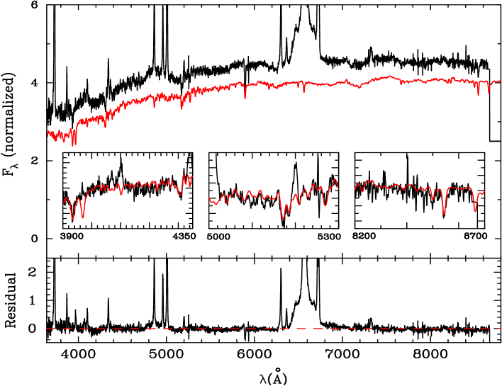
Figure 1.— Sample fit of the synthetic population model for SDSS J081700.40+34556.34. The top panel is the logarithm of the observed spectrum (top black curve) and the synthetic spectra (bottom red curve)(shifted down for clarity). In this top panel, we also show the region around Ca H+K $\lambda\lambda$ 3969, 3934 and G-band (left); the region around Mg Ib$\lambda\lambda$ 5167, 5173, 5184 triplet, Fe 5270Å (middle); the region around Ca II$\lambda\lambda$ 8498, 8542, 8662 triplet (right). The residual spectrum is shown in the bottom panel.

Using Interactive Data Language (IDL), we also carefully model the profiles of $[\rm O~{}\sc{III}]$ and H$\beta$ lines. Since the double-peaked profile of the H$\beta$ line and the asymmetric profiles of $[\rm O~{}\sc{III}]$$\lambda\lambda$4959, 5007 lines, seven-gaussian profiles are used to model these lines carefully, two broad and one narrow components for H$\beta$ plus two sets of one broad and one narrow components for $[\rm O~{}\sc{III}]$$\lambda\lambda 4959,5007$. We take the same linewidth for each component of $[\rm O~{}\sc{III}]$$\lambda\lambda 4959,5007$, fix the flux ratio of $[\rm O~{}\sc{III}]$$\lambda$4959 to $[\rm O~{}\sc{III}]$$\lambda$5007 to be 1:3, and set their wavelength separation to the laboratory value. And we also set the wavelength separation between the narrow component of H$\beta$ and the narrow $[\rm O~{}\sc{III}]$$\lambda$5007 to the laboratory value. We do the lines fitting for these 54 stellar-light subtracted spectra. For spectra without obvious stellar features, we do the emission lines fitting for the extinction-corrected rest-frame SDSS spectra without stellar-light subtraction. At last we obtain the gaseous velocity dispersion, $\sigma_{g}$, from the core $[\rm O~{}\sc{III}]$$\lambda 5007$ line, the total flux of $[\rm O~{}\sc{III}]$$\lambda 5007$ line and the monochromatic flux at 5100Å. Our emission-line profile fitting for SDSS J022014.57-072859.30 is shown in Fig. 2.

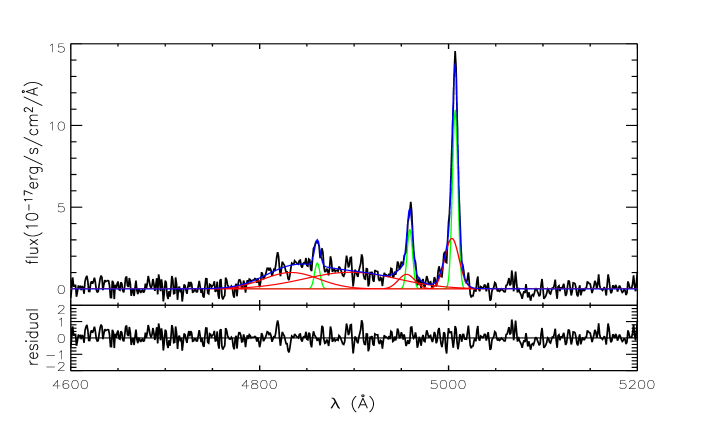
Figure 2.— Sample multi-component fitting of the $[\rm O~{}\sc{III}]$$\lambda\lambda$4959, 5007 lines for SDSS J022014.57-072859.30: composite profile(blue curves); narrow components (green curves); broad components (red curves); the residue (bottom panel).

4. The Masses and the Eddington ratios

4.1. The stellar velocity dispersions

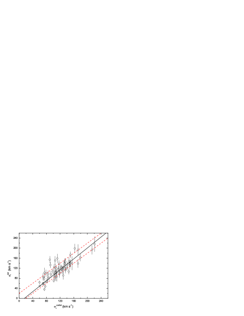
Figure 3.— Comparison of our $\sigma_{*}$ from the partial SDSS spectra with that for a sample of the local AGNs presented by Greene & Ho (2006a). The solid line denotes our best linear fit, the red dash lines are $y=x\pm 20$ km s^-1 . Considering the error bar of $\sigma_{*}$ presented by Greeene & Ho (2006a), most of local AGNs are located between two red dash lines.

In the synthesis, we focus on the strongest stellar absorption features, such as CaII K, G-band, and Ca II$\lambda\lambda$ 8498, 8542, 8662 triplet, which are less affected by emission lines. We put twice more weight for these features during the stellar population synthesis. After correcting the template and the SDSS instrumental resolution, we obtain the value of $\sigma_{*}$ through the direct-fitting method.

Cid Fernandes et al. (2005) applied the same synthesis method to a larger sample of 50,362 normal galaxies from the SDSS Data Release 2 (DR2). Their $\sigma_{*}$ is consistent very well with that of the MPA/JHU group (Kauffmann et al. 2003), the median of the difference is just 9 km s^-1 . They also gave the $\sigma_{*}$ uncertainty based on the S/N (see Table 1 in Cid Fernandes et al. 2005). Typically, the $\sigma_{*}$ uncertainty based on S/N at 4020Å is about: 24 km s^-1 at S/N=5; 12 km s^-1 at S/N=10; 8 km s^-1 at S/N=15. In order to use the typical errors suggested by Cid Fernandes et al. (2005), we calculate the S/N and the starlight fraction at 4020Å. The S/N is the mean flux divided by the root mean square (RMS) of the flux in the range 4010 to 4060 Å. We also performed the method of Cid Fernandes et al. (2005) to compute the S/N by using the SDSS error spectrum, the results are almost the same. Considering the contribution from featureless continuum (FC, represented by a power law), we use an effective S/N to show the typical error of $\sigma_{*}$, where the effective S/N is roughly the S/N multiplied by the stellar fraction. We use the featureless continuum fraction as the up limit of nuclei contribution, because the featureless continuum can be attributed either by a young dusty starburst, by an AGN, or by these two combination (Cid Fernandes et al. 2004). Therefore, the effective S/N is the low limit. In our sample, the effective mean spectral S/N at 4020Å for these objects are 7.2 (see Table 1). Thus the typical uncertainty in $\sigma_{*}$ should be around 20 km s^-1 . For 13 objects with effective S/N less than 5, their $\sigma_{*}$ in Table 1 are preceded by colons.

Here, we also apply this synthesis method to a sample of the local AGNs presented by Greene & Ho (2006a). Greene & Ho (2006a; 2006b) performed a research on the systematic bias of $\sigma_{*}$ derived from the regions around CaII triplet, MgIb triplet, and CaII H+K, respectively (Barth et al. 2002). They argued that the CaII triplet provide the most reliable measurements of $\sigma_{*}$ and there is a systematic offset between $\sigma_{*}$ from CaII K line and that from other spectral regions. We use our synthesis method to their sample in two manners: one is using whole spectrum, the other is just using partial spectrum between 3200Å and 7500Å at the rest frame. We put twice more weight for the strongest absorption features of Ca H+K $\lambda\lambda$ 3969, 3934, G-band, and Ca II$\lambda\lambda$ 8498, 8542, 8662 triplet. We find that the values of $\sigma_{*}$ in these two manners are similar by performing our synthesis method. By using the least-square regression, the best fit between the $\sigma_{*}$ from these two manners ($\sigma^{\rm whole}_{*}$ and $\sigma_{*}^{\rm partial}$, respectively) is: $\sigma^{\rm whole}_{*}=(5.49\pm 3.29)+(0.95\pm 0.03)\sigma_{*}^{\rm partial}$. The spearman coefficient $R$ is 0.97, with a probability of $p_{\rm null}<10^{-4}$ for rejecting the null hypothesis of no correlation.

Because the SDSS spectral coverage is from 3800Å to 9200Å, most of double-peaked AGNs with redshift larger than 0.083 will not cover the range of CaII triplet. For those sources with redshift larger than 0.083, we used the above formula to obtain the corrected velocity dispersion, i.e. $\sigma^{\rm c}_{*}=(5.49\pm 3.29)+(0.95\pm 0.03)\times\sigma_{*}$. The corrected velocity dispersion is listed in Col. (8) in Table 1. And we find that the corrected velocity dispersion is almost the same to the uncorrected one. The largest difference is about 10 km s^-1 , which is less than the typical error of 20km s^-1 .

Based on the SDSS instrumental resolution, we take 60 km s^-1  as a lower limit of $\sigma_{*}$ (e.g. Bernardi 2003). Only for two objects, SDSS J133433.24 -013825.41 and SDSS J214555.03 +121034.17, the measured $\sigma_{*}$ are below/near the lower limit (51 km s^-1 and 62 km s^-1 , respectively). These two objects are excluded from further analysis.

The $\sigma_{*}$ value from the partial SDSS spectra is also used to compare our result with Greene & Ho (2006a), who fitted the region around CaII triplet directly. In Fig. 3, we compared our $\sigma_{*}$ with theirs. We found that the agreement is quite good, the $\sigma_{*}$ difference ($\sigma_{*}^{\rm GH}-\sigma_{*}^{\rm partial}$) distribution is -2.1 km s^-1  with a standard deviation (SD) of 22.7 km s^-1 . By using the least-square regression considering the errors of $\sigma_{*}^{\rm GH}$, the best fit between $\sigma^{\rm GH}_{*}$ and $\sigma_{*}^{\rm partial}$ is: $\sigma^{\rm GH}_{*}=(-16.66\pm 3.56)+(1.09\pm 0.04)\sigma_{*}^{\rm partial}$ (solid line in Fig. 3). The spearman coefficient $R$ is 0.86, the standard deviation is 2.11, with $p_{\rm null}<10^{-4}$.

4.2. The Results

For these double-peaked AGNs with reliable $\sigma^{c}_{*}$, we use the $M_{\rm bh}-\sigma_{*}$ relation to derive the SMBH mass (e.g. Tremaine et al. 2002 and reference therein),

$$M_{\rm bh}(\sigma_{*}^{c})=10^{8.13}\left(\frac{\sigma_{*}^{c}}{200~{}\rm km~{}s^{-1}}\right)^{4.02}~{}~{}M_{\odot}.$$ (3)

We calculate the Eddington ratio, e.g., the ratio of the bolometric luminosity ($L_{\rm bol}$) to the Eddington luminosity ($L_{\rm Edd}$), where $L_{\rm Edd}=1.26\times 10^{38}(M_{\rm bh}/M_{\odot})\ \rm erg~{}s^{-1}$. We use the monochromatic luminosity at 5100Å ($\lambda L_{\lambda}$ at 5100Å) to estimate the bolometric luminosity, $L_{\rm bol}=c_{\rm B}\lambda L_{\lambda}$(5100Å), where $c_{\rm B}=9$ (Kaspi et al. 2000). These results are presented in Table 1.

For the typical uncertainty of 20 km s^-1  for $\sigma_{*}=200$ km s^-1 , the error of $\log~{}\sigma_{*}$ would be about 0.05 dex, corresponding to 0.2 dex for $\log M_{\rm bh}$. The error of $\log M_{\rm bh}$ is about 0.4 considering the error of 0.3 dex form the $M_{\rm bh}-\sigma_{*}$ relation (Tremaine et al. 2002). Richards et al. (2006) suggested a bolometric correction factor of $10.3\pm 2.1$ at 5100 Å. Therefore, the final Eddington ratio, $L_{\rm bol}/L_{\rm Edd}$, has a large uncertainty, about 0.5 dex.

Figure 4.— The histograms of the black hole masses (left) and the Eddington ratios (right) for these 52 double-peaked AGNs with reliable $\sigma^{c}_{*}$.

In Fig. 4, we show the histograms of the black hole masses and the accretion ratios for these 52 double-peaked AGNs. The black hole masses range from $1.0\times 10^{7}$ to $5.5\times 10^{8}$ $M_{\odot}$ with a mean value of $\log M_{\rm bh}/M_{\odot}=7.76\pm 0.37$. Using the H$\alpha$ FWHM and the 5100Å monochromatic luminosity, Wu & Liu (2004) estimated the SMBH masses and the Eddington ratios for an assembled double-peaked AGNs sample. Lewis & Eracleous (2006) noted that the BH masses from the H$\alpha$ FWHM are not completely consistent with those from the stellar velocity dispersion. Our BH masses derived from $\sigma^{c}_{*}$ are indeed smaller than those from the H$\alpha$ FWHM (Wu & Liu 2004) by about an order of magnitude. This will lead to our $L_{\rm bol}/L_{\rm Edd}$ larger than that from the H$\alpha$ FWHM by almost an order of magnitude.

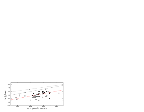
Figure 5.— The BLRs sizes versus the monochromatic luminosity at 5100Å (where $f$=0.75 for random BLRs orbits). Objects with effective S/N in 4020 Å  less then 5 is denoted as open stars. The black dash line is the empirical size-luminosity relation, $R_{\rm BLR}=22.3\times[\lambda L_{\lambda}$(5100Å)$/10^{44}~{}\rm ergs^{-1}]^{0.69}~{}\rm lt-days$, found by Kaspi et al. (2005). The black dot line is the empirical size-luminosity relation,$R_{\rm BLR}=40\times(\lambda L_{\lambda}$(5100Å)$/10^{44}~{}\rm ergs^{-1})^{0.52}~{}\rm lt-days$, found by Bentz et al. (2006). The red solid line is our best fit with the fixed slope of 0.69 ($R$=0.29), lower by -0.63 dex respect to dash line.

The Eddington ratio has a distribution with mean and the standard deviation of $\log(L_{\rm bol}/L_{\rm Edd})$ is $-1.13\pm 0.38$. It is suggested that the accretion disk in double-peaked AGNs is in the mode of Advection Dominated Accretion Flow (ADAF) (e.g. Eracleous & Halpern 2003). When the Eddington ratio is below than the critical one $L_{\rm Bol}/L_{\rm Edd}\sim 0.0028\alpha_{0.1}^{2}$ (Mahadevan 1997), the ADAF appears, where $\alpha_{0.1}=\alpha/0.1$ is viscous coefficient. For our SDSS sample, all objects have Eddington ratios larger than this critical value of 0.0028. The present results from Fig. 4 clearly show that these double peaked AGNs have accretion disks in the standard regime.

The black hole masses can be independently tested by the relation between the black holes and bulges. The Appendix gives details of the test. We find the black hole masses are consistent from $M_{\rm bh}-M_{\rm bulge}$ and $M_{\rm bh}-\sigma_{*}$ relations.

5. BLRs in double-peaked AGNs

5.1. The size of BLRs

We also calculate the BLRs sizes for these 52 double-peaked AGNs using the SMBHs masses derived from $\sigma_{*}^{c}$ and the H$\alpha$ FWHM. We firstly transform the H$\alpha$ FWHM to the H$\beta$ FWHM by (Greene & Ho 2005b):

$$\rm FWHM_{\rm H\beta}=(1.07\pm 0.07)\times 10^{3}\left(\frac{\rm FWHM_{\rm H\alpha}}{10^{3}~{}\rm kms^{-1}}\right)^{(1.03\pm 0.03)}~{}{\rm kms^{-1}}.$$ (4)

From the SMBH masses derived from the velocity dispersions, we can calculate the BLRs sizes:

$$R_{\rm BLR}=\frac{M_{\rm bh}(\sigma_{*}^{c})\times 5.123}{f\times\rm FWHM_{H\beta}^{2}}~{}~{}~{}~{}~{}~{}~{}~{}~{}~{}\rm lt-days,$$ (5)

where $f$ is the scaling factor related to the kinematics and geometry of the BLRs, defined by $M_{\rm bh}=f\frac{R_{\rm BLR}V_{\rm p}^{2}}{G}$, $V_{\rm p}$ is the Keplerian velocity in disk plane. For random orietation of BLR cloud Keplerian orbits, $f$ is 0.75.

In Fig. 5, we plot the BLRs sizes versus the monochromatic luminosity at 5100Å (assuming $f$=0.75 for random BLRs orbits). Almost all objects are located below the empirical size-luminosity relation (black dash line) found by Kaspi et al. (2005). The correlation between the BLRs sizes and the monochromatic luminosity at 5100Å is not too strong. The best fit is shown as red solid line in Fig. 5 as $R_{\rm BLR}=5.1\left[\lambda L_{\lambda}(5100\AA)/10^{44}~{}{\rm ergs^{-1}}\right]^{0.69}$ lt-days ($R=0.34$, $P_{\rm null}=0.20$), lower by -0.64 dex respecting to the empirical relation found by Kaspi et al. (2005). When excluding objects with effective S/N in 4020 Å less then 5 (open stars in Fig. 5), for fixed slope of 0.69, the best fit gives almost the same line but with a smaller $R$ of $0.28$.

If we used $f$=0.52 (Table 2 in Collin et al. 2006), $\log R$ will increased by 0.16 dex, the BLRs sizes of double-peaked AGNs are still deviated from the empirical relation found by Kaspi et al. (2005) (about 0.48 dex). FWHMs of the double-peaked AGNs are about twice as broad as other AGN of similar luminosity (Eracleous & Halpern 1994, 2003; Strateva et al. 2003). If the double-peaked AGNs are not systematically more massive than other AGNs, equation 5 suggested that BLRs radii can be smaller than for a similarly massive ”normal” AGNs by a factor of 4.

We have to point out that here we are not really testing the $R_{\rm BLR}-L$ relation in double peaked AGNs, but the comparison with $R_{\rm BLR}-L$ relation allows us to derive the factor $f$.

5.2. The factor $f$, BLR inclinations and Non-virial BLRs

If we use the empirical $R_{\rm BLR}-L$ relation (Kaspi et al. 2005) to derive the $R_{\rm BLR}$ and the SMBH masses, $M_{\rm bh}(\sigma_{*}^{c})$, to do the calibration of the factor $f$ (Onken et al. 2004), we find that the distribution of $f$ is 0.179 with a standard deviation of 0.171. It is not consistent with the value of $\langle f\rangle=5.5/4$ presented by Onken et al. (2004) and it is about 1/3 of $0.52\pm 0.13$ suggested by Collin et al. (2006). Our results suggest that the empirical relation between the BLRs sizes and the luminosity at 5100Å does not hold for double-peaked AGNs (see also Zhang et al. 2007), otherwise the calibration factor $f$ should be as low as 0.179. An important consequence of the breakdown in the size-luminosity relationship is that using mass estimation methods based on the size-luminosity relationship and the calibration factor of 0.75 can lead to an order of magnitude over-estimate of the SMBH mass (Wu & Liu 2004).

If BLRs are disk-like with an inclination of $\theta$, the relation between the H$\beta$ FWHM and the Keplerian disk plane velocity, $v_{\rm p}$, is given by (Wills & Browne 1986)

$${\rm FWHM_{\rm H\beta}}=2\left(V_{\rm r}^{2}+V_{\rm p}^{2}\sin^{2}\theta\right)^{1/2},$$ (6)

where $V_{\rm r}$ is the random isotropic component. We may derive the scaling factor as $f=1/[4(V_{\rm r}/V_{\rm p})^{2}+4\rm sin^{2}\theta]$. Ignoring $V_{\rm r}$, $f=1/(\rm 2sin\theta)^{2}$, and the minimum of $f$ is 0.25. For only ten object with $f>0.25$, we can derive the inclination of $\theta$ by the above formula. The mean inclination is 56 degrees. It is suggested that double-peaked AGNs are not preferentially edge-on (Eracleous & Halpern 1994, 2003; Strateva et al. 2003), most have an inclination of less than 50 degrees. If all these objects were nearly edge-on, the obscuring torus would prevent us from seeing the broad lines. Collin et al. (2006) suggested that objects with large FWHMs, inclination effects are not really important. In these 52 double-peaked AGNs, 42 objects have smaller $f$ less than 0.25. $V_{\rm r}$ can’t be omitted, we need to consider the random isotropic component, implying the non-virial dynamics of BLRs in double-peaked AGNs. If we use $f$ to trace the non-virial effect, smaller $f$ means strong non-virial effect. We find $f$ have strong correlations with $\log M_{\rm bh}$ and $\log(L_{\rm bol}/L_{\rm Edd})$ (see Fig. 6). Using the least-square regression, we derive the correlations are:

$$\log f=(-1.63\pm 0.12)-(0.65\pm 0.10)\log(L_{\rm bol}/L_{\rm Edd}),$$ (7)

where $R=-0.69$, $p_{\rm null}<10^{-4}$; and

$$\log f=(-4.31\pm 0.97)+(0.44\pm 0.13)\log M_{\rm bh}/M_{\odot},$$ (8)

where $R=0.45$ with $p_{\rm null}=9.6\times 10^{-4}$. When we exclude objects with effective S/N in 4020 Å less then 5 (open stars in Fig. 6), the best fits for $f$ relations between SMBH mass and the Eddington ratio give a little larger $R$ ($-0.75,0.52$, respectively). We should note that the reason of these strong correlations are that $f$ is derived from $M_{\rm bh}$, $R_{\rm BLR}$ [from $\lambda L_{\lambda}(5100\AA)$ ], and $\rm FWHM_{H\beta}$. These strong correlations suggest that objects with larger Eddington ratios have strong non-virial effect.

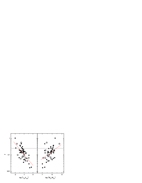
Figure 6.— The scaling factor $f$ versus the Eddington ratio (left panel) and the SMBH masses (right panel). Objects with effective S/N in 4020 Å  less then 5 is denoted as open stars. The dash lines are $f=0.25$. The correlation coefficient for the relation between the peak separation and the Eddington ratio is $R=-0.69$ and that between the separation and the black hole mass is $R=0.45$.

3C 390.3 is the only double peaked object with the direct measurements of the time delay and the host stellar velocity dispersion. And it locates in the empirical relation between BLRs sizes and the luminosity (e.g. Kaspi et al. 2005). By $\sigma_{*}$ of 240 km s^-1 (Onken et al. 2004), we find that $f$ is about 1.3, consistent with the assumption of random BLRs orbits in 3C390.3. Its small Eddington ratio (Lewis & Eracleous 2006), $(2-4)\times 10^{-2}$, is also consistent with the virial BLRs dynamics (See Fig. 6).

6. Peak separation, BH Mass and Eddington ratio

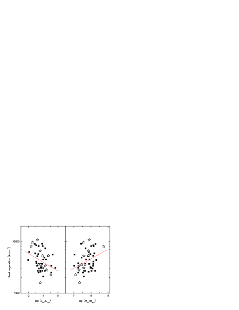
Figure 7.— The peak separation versus the Eddington ratio (left panel) and the SMBH masses (right panel). Objects with effective S/N in 4020 Å less then 5 is denoted as open stars. The correlation coefficient for the relation between the peak separation and the Eddington ratio is $R=-0.33$, which is almost the same for that between the separation and the black hole mass ($R=0.35$).

For double-peaked AGNs, the peak separation, $\Delta v=\lambda_{\rm red}-\lambda_{\rm blue}$, has a large variance ranging from about 1000 km s^-1  to about 10000 km s^-1  (Table 3 in Strateva et al. 2003). In Fig. 7, we show the relations between $\log\Delta\lambda$ and $\log(L_{\rm bol}/L_{\rm Edd})$, $\log M_{\rm bh}$. Using the least-square regression, we derive the correlation between $\log\Delta v$ and $\log(L_{\rm bol}/L_{\rm Edd})$ to be:

$$\log\Delta v=(3.43\pm 0.08)-(0.17\pm 0.06)\log(L_{\rm bol}/L_{\rm Edd}),$$ (9)

where $R=-0.33$, $p_{\rm null}=0.017$ (see Fig. 7). For the relation between $\log\Delta\lambda$ and $\log M_{\rm bh}$,

$$\log\Delta v=(2.17\pm 0.55)+(0.11\pm 0.08)\log(M_{\rm bh}/M_{\odot}),$$ (10)

where $R$ is 0.35 with $p_{\rm null}=0.011$. When excluding objects with effective S/N in 4020 Å less then 5 (open stars in Fig. 7), the best fits for $\log\Delta v$ relations between SMBH mass and the Eddington ratio give smaller $R$ ($-0.22,0.21$, respectively). We also do the multiple regression for the dependence of $\Delta v$ on $\log(L_{\rm bol}/L_{\rm Edd})$ and $\log M_{\rm bh}$,

$$\log\Delta v=(2.54\pm 0.64)+(0.13\pm 0.09)\log(M_{\rm bh}/M_{\odot})$$ (11)

$$-(0.10\pm 0.09)\log(L_{\rm bol}/L_{\rm Edd}),$$

where the $R-$Square correlation coefficient is 0.15.

Wu & Liu (2004) also studied this correlation and obtained an apparent stronger correlation ($R=0.84$). Their derived strong correlation is mainly due to the very strong correlation between the separation and the H$\alpha$ FWHM ($R=0.88$). When the H$\alpha$ FWHM is fixed, they found that the partial correlation coefficient is only 0.05. In this paper, we use the stellar velocity dispersion to estimate the black hole masses, and we also find a mild correlation between $\Delta v$ and $L_{\rm bol}/L_{\rm Edd}$, which implies that the peak separation would be smaller for AGNs with higher Eddington ratios. It provides clues to why previous double-peaked AGNs have lower Eddington ratios.

There is increasing evidence for a disk geometry of the BLR (see a review of Laor 2007). If we assume that peak separation is created by the doppler shift of the movement of a thin annulus and the annulus radius corresponds the location where the self-gravitation domiantes (Bian & Zhao 2002), we have the radius $R_{\rm SG}/R_{g}=3586m_{8}^{-2/9}\dot{m}^{4/9}\alpha^{2/9}$ (their eq. 18 in Laor & Netzer 1989), where $R_{g}=1.5\times 10^{13}m_{8}$ cm, $m_{8}=M_{\rm bh}/10^{8}M_{\odot}$, $\dot{m}$ is the Eddington ratio and $\alpha$ is the viscosity. The maximum separation of the double peaks in units of Å under the edge-on orientation to an observer is given

$$\Delta\lambda=\lambda_{0}\left(\frac{R_{\rm g}}{R_{\rm SG}}\right)^{1/2}=84.9~{}\alpha_{0.1}^{-1/9}\dot{m}^{-2/9}m_{8}^{1/9}~{}\AA,$$ (12)

where we use the peak separation in term of separation velocity,

$$\Delta v=7.76\times 10^{3}~{}\alpha_{0.1}^{-1/9}\dot{m}^{-2/9}m_{8}^{1/9}~{}{\rm km\ s}^{-1}.$$ (13)

where $\alpha_{0.1}=\alpha/0.1$ and H$\alpha$ wavelength $\lambda_{0}=6563$Å.

Considering the uncertainties of the fitting results for the peak separation correlations with SMBH mass and the Eddington ratio, the slopes are consistent with the simple theoretical expectation. We have to stress that equation (11) is for the maximum separation (edge-on orientation) when the disk structure is given. More sophisticated model is needed for explanations of the dependence of peak separations and Eddington ratios. The scatters in Fig 7 may be caused by different orientation of the BLR in the sample.

We also find no significant correlations between the ratio of the red peak height to the blue height and the Eddington ratio, the black hole mass, the peak separation. Since the Keplerian velocity is much below the light speed, the Doppler boosting effects could be hidden by complex situations of the BLR.

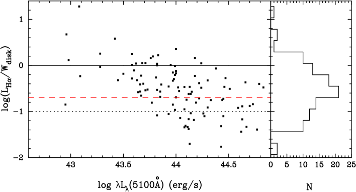
Figure 8.— The ratio of the H$\alpha$ line luminosity ($L_{\rm H\alpha}$) to the line-emitting power ($W_{\rm disk}$) versus the monochromatic luminosity at 5100Å ($\log\lambda L_{\lambda}$(5100 Å)). The solid line is $L_{\rm H\alpha}=W_{\rm disk}$, the dash line is $L_{\rm H\alpha}=0.2W_{\rm disk}$, and the dot line is $L_{\rm H\alpha}=0.1W_{\rm disk}$. We display the histogram of the distribution of $L_{\rm H\alpha}/W_{\rm disk}$ (right).

7. Energy budget

Here we discuss the energy budget of the line-emitting accretion disk. Based on the standard accretion disk model, the disk radiation as a function of radius $\xi$ is (Chen et al. 1989):

$$F(\xi)=1\times 10^{12}m_{8}^{-2}\dot{M}_{24}\xi_{100}^{-3}[1-(6/\xi)^{1/2}]~{}\rm ergs~{}cm^{-2}~{}s^{-1}$$ (14)

where $m_{8}=M_{\rm bh}/10^{8}M_{\odot}$, $\dot{M}_{24}$ is the accretion rate in units of $10^{24}~{}g~{}s^{-1}$, and the dimensionless radius $\xi_{100}$ is $\xi/(100R_{g})$. Using $\dot{M}=L_{\rm bol}/(\zeta c^{2})$ where the efficiency $\zeta$ is 0.1, the gravitational power output of the line-emitting disk annulus between $\xi_{1}$ and $\xi_{2}$ is (Eracleous & Halpern 1994):

$$W_{\rm disk}(\xi_{1},\xi_{2})=7.7\times L_{\rm bol}~{}~{}~{}~{}~{}~{}~{}~{}~{}~{}~{}~{}~{}~{}~{}~{}~{}~{}~{}$$

$$\left[\frac{1}{\xi_{1}}\left(1-{\sqrt{\frac{8}{3\xi_{1}}}}\right)-\frac{1}{\xi_{2}}\left(1-\sqrt{\frac{8}{3\xi_{2}}}\right)\right]{\rm ergs~{}s^{-1}},$$ (15)

where $L_{\rm bol}$ is in units of $\rm erg~{}s^{-1}$. It is noted that $W_{\rm disk}$ is independent of the black hole mass, when we use the typical radius in units of $R_{g}$. We use the luminosity at 5100Å to calculate the bolometric luminosity. From the work of Eracleous & Halpern (2003) and Strateva et al. (2003), the inner radius is about hundreds of $R_{\rm g}$, and the outer radius is about thousands of $R_{\rm g}$. The outer radius of line-emitting accretion disk is about near the inner position of torus. We can assume typical inner and outer radii of $\xi_{1}=450R_{g}$ and $\xi_{1}=3000R_{g}$ to calculate the energy output for these double-peaked SDSS AGNs, i.e. $W_{\rm disk}=10^{-1.876}\times L_{\rm bol}\ \rm erg~{}s^{-1}$. The distribution of $\rm{log}(L_{\rm H\alpha}/W_{\rm disk})$ is $-0.55\pm 0.06$ with the standard deviation of 0.57 (see also Fig. 8). If assuming as much as $20\%$ of the power was radiated as H$\alpha$ line (dashed line in Fig. 8), our results show that only 36 out of 105 double-peaked AGNs would generate enough power to produce observed strength of H$\alpha$ emission. If we adopt the value of 10%, more objects (83 out of 105 objects) showed the energy problem. It implied that the majority of double-peaked AGNs need external illumination of the disk (e.g. an inner iron torus or corona) to produce the observed strength of H$\alpha$ line (Strateva et al. 2006; Cao & Wang 2006).

8. conclusions

We use the simple population synthesis to model the stellar contributions in double-peaked SDSS AGNs. The reliable stellar velocity dispersions are obtained for 52 medium-luminous double-peaked SDSS AGNs with obvious stellar features. We find that: 1) The black hole mass is from $1.0\times 10^{7}M_{\odot}$ to $5.5\times 10^{8}M_{\odot}$ and the Eddington ratio is from about 0.01 to about 1; 2) The factor $f$ far deviates from the virialized value 0.75, suggesting the non-virial dynamics of BLRs; 3) The peak separation is mildly correlated with the Eddington ratio and SMBH mass with almost the same correlation coefficients, which can be interpreted in the doppler shift of thin annulus of BLRs created by gravitational instability; 4) Based on the line-emitting accretion disk model, we need external illumination of the accretion disk to produce the observed strength of H$\alpha$ line. In the future, using different models, we would fit the double-peaked profiles to constrain the nature of double-peaked AGNs. We can also use the double-peaked AGNs to constrain the BLRs origin ( Nicastro 2000; Laor 2003; Bian & Gu 2007).

Appendix A The relation between the host mass and the SMBH mass

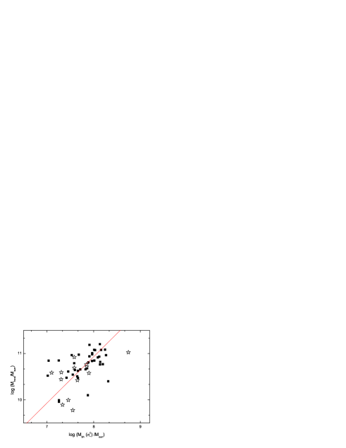
Figure 9.— The relation between the host mass and the SMBH mass. With fixed slope of 1, the solid line denotes the best fit with $R$=0.53 and $p_{\rm null}<10^{-4}$. Objects with effective S/N in 4020 Å less then 5 is denoted as open stars.

For the sample of 52 double-peaked SDSS AGNs, assuming $\lambda L_{\lambda}\propto\lambda^{0.5},\lambda L_{\lambda}(5100\AA)$ is translated to $\lambda L_{\lambda}(5530\AA)$. The host luminosity in V band is the value of $\lambda L_{\lambda}(5530\AA)$ multiplied by the stellar fraction at 5530Å. We assume that the host luminosity in V band approximates the bulge luminosity $L_{\rm bulge}$ in V-band. We then use the following formula to calculate the bulge mass: $\log(M_{\rm bulge}/M_{\odot})=1.18\log(L_{\rm bulge}/L_{\odot})-1.11$ (Magorrian et al. 1998). Fig. 9 shows this bulge mass versus the BH mass from $\sigma_{*}$. We fit with fixed slope as 1, intercept is $2.93\pm 0.05$, correlation coefficient is 0.53. The null hypothesis is less then $10^{-4}$. We find that the $M^{\rm bulge}_{V}$ versus the $\log\sigma$ relation is consistent with Fig.4 of Faber et al. 1997. Therefore, the SMBH mass from $L_{\rm bulge}$ and the Magorrian relation agrees with that from $\sigma_{*}$. When we exclude objects with effective S/N in 4020 Å less then 5 (open stars in Fig. 9), for fixed slope of 1, the best fit gives that intercept is $2.95\pm 0.05$, correlation coefficient is 0.49.

It is suggested that the mass from the $M_{\rm bh}-\sigma_{*}$ relation could underestimate the SMBH mass for the massive ellipticals with SMBH mass larger than $10^{9}M_{\odot}$ (Fig. 2 in Lauer et al. 2007). For our 52 double-peaked AGNs, their SMBH masses are all less than $10^{9}M_{\odot}$ from $M_{\rm bh}-M_{\rm bulge}$ relation. The present results are less affected by Lauer et al’s findings.

Table 1Results for 52 double-peaked AGNs.

Name	z	EW(Ca K)	$\chi^{2}$	FC	S/N	$\sigma_{*}$	$\sigma_{*}^{\rm c}$	$\sigma_{\rm g}$	$\lambda L_{\lambda}(5100\AA)$	$M_{\rm bh}$	$L_{\rm bol}/L_{\rm Edd}$	$\Delta V$
(1)	(2)	(3)	(4)	(5)	(6)	(7)	(8)	(9)	(10)	(11)	(12)	(13)
SDSS J000815.46$-$104620.57	0.199	$-3.5\pm 1.3$	0.86	0.45	4.12	:148.30	146.37	$112.2\pm 4.6$	43.71	7.59	-1.02	3100
SDSS J011140.03$-$095834.94	0.207	$-3.7\pm 0.7$	0.91	0.58	3.49	:110.93	110.87	$92.5\pm 31.1$	43.77	7.10	-0.48	2300
SDSS J013407.88$-$084129.98	0.070	$-7.7\pm 0.6$	1.07	0.07	9.47	121.14	121.14$\star$	$84.8\pm 1.3$	42.95	7.25	-1.45	3800
SDSS J014901.08$-$080838.23	0.210	$-3.1\pm 7.0$	1.05	0.64	2.78	:125.25	124.48	$169.9\pm 5.3$	43.67	7.30	-0.77	2800
SDSS J023253.42$-$082832.10	0.265	$-2.7\pm 0.6$	0.86	0.30	11.00	186.03	182.22	$236.1\pm 14.3$	43.97	7.97	-1.14	3200
SDSS J024052.82$-$004110.93	0.247	$-3.0\pm 0.3$	1.31	0.67	7.52	121.61	121.02	$105.9\pm 3.9$	44.22	7.25	-0.18	3100
SDSS J024703.24$-$071421.59	0.333	$-4.3\pm 2.3$	0.81	0.62	3.41	:293.48	284.29	$402.1\pm 19.0$	44.08	8.74	-1.81	8100
SDSS J024840.03$-$010032.68	0.184	$-4.7\pm 1.5$	0.72	0.38	6.26	155.34	153.06	$91.9\pm 0$	43.62	7.66	-1.19	2700
SDSS J025220.89$+$004331.32	0.170	$-1.3\pm 0.2$	1.01	0.50	6.81	174.65	171.41	$195.7\pm 6.9$	43.82	7.86	-1.18	2600
SDSS J025951.71$-$001522.78	0.102	$-2.5\pm 0.5$	0.90	0.62	4.51	:137.38	136.00	$116.1\pm 19.3$	43.28	7.46	-1.33	3600
SDSS J034931.03$-$062621.05	0.287	$-5.1\pm 0.8$	0.98	0.61	4.32	:148.31	146.38	$155.0\pm 9.2$	44.09	7.59	-0.64	5300
SDSS J081700.40$+$343556.34	0.062	$-7.6\pm 1.5$	1.33	0.16	9.35	172.92	172.92$\star$	$200.8\pm 4.3$	43.08	7.88	-1.94	6300
SDSS J081916.28$+$481745.48	0.223	$-2.6\pm 0.4$	1.06	0.61	4.84	:173.85	170.65	$170.6\pm 166.4$	43.97	7.85	-1.03	5400
SDSS J082133.60$+$470237.33	0.128	$-7.9\pm 2.9$	0.90	0.19	9.47	171.11	168.05	$172.8\pm 6.5$	43.58	7.83	-1.39	5200
SDSS J084535.37$+$001619.52	0.260	$-5.2\pm 1.8$	0.77	0.33	6.52	106.66	106.82	$113.3\pm 9.5$	43.82	7.04	-0.36	5600
SDSS J091459.05$+$012631.30	0.198	$-3.2\pm 0.3$	0.80	0.33	11.38	156.94	154.59	$180.7\pm 15.5$	43.97	7.68	-0.86	7400
SDSS J092515.00$+$531711.91	0.186	$-3.9\pm 0.7$	0.79	0.26	8.78	203.50	198.82	$142.7\pm 11.1$	43.85	8.12	-1.42	3400
SDSS J100443.43$+$480156.45	0.199	$-5.6\pm 1.5$	1.00	0.52	3.92	:172.93	169.77	$115.2\pm 3.3$	43.79	7.84	-1.20	6600
SDSS J101405.89$+$000620.36	0.141	$-7.6\pm 1.1$	1.50	0.26	12.21	221.51	215.92	$166.8\pm 6.5$	43.85	8.26	-1.56	9000
SDSS J103202.41$+$600834.47	0.294	$-2.7\pm 1.0$	0.82	0.55	5.30	179.60	176.11	$164.1\pm 8.1$	43.98	7.91	-1.08	3700
SDSS J104108.18$+$562000.32	0.230	$-3.5\pm 0.9$	1.04	0.43	6.20	205.50	200.72	$181.9\pm 0.2$	43.82	8.14	-1.47	8500
SDSS J104128.60$+$023204.99	0.182	$-4.6\pm 0.5$	0.91	0.27	9.75	185.68	181.88	$191.1\pm 26.2$	43.78	7.96	-1.33	5700
SDSS J104132.78$-$005057.46	0.303	$-3.1\pm 0.3$	1.41	0.47	10.42	179.70	176.20	$195.1\pm 4.2$	44.24	7.91	-0.81	4500
SDSS J110742.76$+$042134.18	0.327	$-2.5\pm 0.6$	0.99	0.42	6.12	205.09	200.32	$251.5\pm 13.6$	44.18	8.13	-1.10	3700
SDSS J113021.41$+$005823.04	0.132	$-6.9\pm 1.0$	0.98	0.31	10.85	148.10	146.19	$95.2\pm 0.9$	43.73	7.58	-1.00	2100
SDSS J113633.08$+$020747.65	0.239	$-4.2\pm 0.3$	1.18	0.74	6.41	143.45	141.76	$163.2\pm 10.2$	44.22	7.53	-0.45	2500
SDSS J114051.58$+$054631.13	0.132	$-11.2\pm 3.9$	0.78	0.41	6.43	134.19	132.97	$138.7\pm 8.5$	43.50	7.42	-1.06	9100
SDSS J115047.48$-$031652.95	0.149	$-5.4\pm 1.1$	0.89	0.46	5.98	137.15	135.78	$91.2\pm 3.7$	43.69	7.45	-0.91	4900
SDSS J122009.55$-$013201.14	0.288	$-5.2\pm 1.2$	0.96	0.49	6.70	186.09	182.28	$179.4\pm 19.5$	44.02	7.97	-1.09	3100
SDSS J130927.67$+$032251.76	0.267	$-2.6\pm 0.5$	1.30	0.36	10.66	199.92	195.42	$256.1\pm 0.5$	43.95	8.09	-1.28	3000
SDSS J132442.44$+$052438.86	0.116	$-8.8\pm 10.4$	1.12	0.45	3.20	:145.40	143.62	$231.7\pm 8.9$	42.98	7.55	-1.72	9700
SDSS J132834.14$-$012917.64	0.151	$-4.2\pm 1.0$	1.41	0.60	4.70	:154.22	152.00	$180.6\pm 2.2$	43.64	7.65	-1.16	3600
SDSS J133312.42$+$013023.73	0.217	$-2.8\pm 0.8$	1.03	0.55	5.18	105.37	105.59	$129.0\pm 2.3$	43.71	7.01	-0.45	3400
SDSS J133338.30$+$041803.94	0.202	$-3.0\pm 0.5$	0.97	0.36	7.34	206.10	201.29	$185.9\pm 16.7$	43.82	8.14	-1.47	4100
SDSS J134617.54$+$622045.47	0.116	$-3.4\pm 0.3$	1.37	0.64	7.94	153.91	151.71	$114.1\pm 1.3$	43.73	7.65	-1.07	—
SDSS J140019.27$+$631426.93	0.331	$-2.3\pm 0.5$	1.05	0.83	5.08	204.44	199.71	$167.1\pm 25.5$	44.59	8.13	-0.69	5300
SDSS J141454.55$+$013358.55	0.269	$-4.1\pm 0.7$	1.15	0.29	10.97	218.93	213.47	$287.8\pm 8.6$	44.03	8.24	-1.36	2700
SDSS J141613.37$+$021907.82	0.158	$-5.9\pm 1.2$	1.02	0.54	6.70	212.96	207.80	$117.6\pm 0.2$	43.81	8.20	-1.54	5900
SDSS J141946.06$+$650353.04	0.148	$-3.7\pm 0.3$	1.18	0.55	8.11	149.36	147.38	$154.9\pm 6.3$	43.85	7.60	-0.90	2700
SDSS J142754.76$+$635448.42	0.145	$-4.2\pm 0.3$	1.39	0.70	7.33	159.98	157.48	$117.2\pm 9.5$	43.86	7.71	-0.99	4500
SDSS J143455.31$+$572345.37	0.175	$-2.0\pm 0.4$	1.65	0.51	10.09	191.25	187.18	$202.6\pm 35.9$	44.00	8.01	-1.17	3100
SDSS J154534.55$+$573625.12	0.268	$-2.2\pm 0.4$	0.92	0.46	9.34	193.04	188.88	$180.6\pm 4.9$	44.12	8.03	-1.05	2700
SDSS J170102.28$+$340400.60	0.094	$-2.7\pm 0.4$	1.62	0.75	3.79	:127.55	126.66	$118.9\pm 1.4$	43.28	7.33	-1.20	1600
SDSS J172102.47$+$534447.29	0.192	$-5.0\pm 2.4$	0.78	0.35	4.45	:125.66	124.86	$138.7\pm 5.6$	43.60	7.31	-0.85	3400
SDSS J210109.58$-$054747.31	0.179	$-6.2\pm 1.4$	0.85	0.32	7.52	177.42	174.04	$168.0\pm 15.1$	43.75	7.89	-1.29	3700
SDSS J214935.23$+$113842.04	0.239	$-9.5\pm 5.7$	0.85	0.56	1.92	:178.69	175.24	$132.8\pm 10.0$	43.66	7.90	-1.38	10800
SDSS J222132.41$-$010928.76	0.288	$-6.3\pm 1.1$	0.84	0.56	5.01	190.63	186.59	$220.5\pm 14.9$	44.12	8.01	-1.03	8200
SDSS J223302.68$-$084349.13	0.058	$-7.2\pm 0.6$	1.68	0.37	10.05	121.19	121.19$\star$	$89.7\pm 0.9$	43.09	7.26	-1.31	2500
SDSS J223336.71$-$074337.10	0.174	$-4.6\pm 0.9$	0.96	0.36	9.12	145.42	143.64	$192.2\pm 16.4$	43.58	7.55	-1.12	3100
SDSS J230545.67$-$003608.55	0.269	$-7.1\pm 2.3$	0.93	0.35	5.52	208.17	203.25	$167.4\pm 9.8$	44.00	8.16	-1.30	8200
SDSS J232721.96$+$152437.31	0.046	$-5.2\pm 0.1$	2.10	0.45	18.59	221.87	221.87$\star$	$165.3\pm 0.4$	43.45	8.31	-2.01	4400
SDSS J235128.77$+$155259.15	0.096	$-2.8\pm 0.2$	1.21	0.66	6.96	155.30	153.03	$112.1\pm 2.9$	43.66	7.66	-1.15	3700

Note. — Col. (1): Object name. Col. (2): Redshift. Col. (3): Equivalent width of Ca K and the error in units of Å. Col. (4): $\chi^{2}$. Col. (5) fraction of featureless continuum component. Col. (6): effective S/N from the S/N at 4020 Å and the fraction of featureless continuum component. Col. (7): Uncorrected stellar velocity dispersion in units of $\rm km~{}s^{-1}$, and values for objects with effective S/N $<5$ are preceded by a colon. Col. (8): Corrected stellar velocity dispersion in units of $\rm km~{}s^{-1}$. For 4 objects with Ca II triplet, it is not need to do the correction, which are shown as $\star$. Col. (9): Corrected gas velocity dispersion in units of $\rm km~{}s^{-1}$. Col. (10): $\log$ of the monochromatic luminosity at 5100 Å in units of $\rm ergs~{}s^{-1}$ . Col. (11): $\log$ of SMBH masses from corrected stellar velocity dispersion in units of $\rm M_{\odot}$. Col. (12): The Eddington ratios. Col. (13): The peak separations in units of $\rm km~{}s^{-1}$.

References

- (1) Abazajian, K., et al. 2005, AJ, 129, 1755
- (2) Barth, A. J., Ho, L. C., Filippenko, A. V., Rix, H., Sargent, W. L. W. 2001, ApJ, 546, 205
- (3) Bentz et al. 2006, ApJ, 644, 133
- (4) Bernardi, M., et al. 2003, AJ, 125, 1817
- (5) Bian, W., Zhao, Y. 2002, A&A, 395, 465
- (6) Bian, W., Zhao, Y. 2004, MNRAS, 347, 607
- (7) Bian, W., Yuan, Q., Zhao, Y. 2005, MNRAS, 364, 187
- (8) Bian, W., Gu, Q, Zhao. Y, Chao, L., Cui, Q. 2006, MNRAS, 372, 876
- (9) Bian, W., Gu, Q. 2007, ApJ, 657, 159
- (10) Bower, G. A., Wilson, A. S., Heckman, T. M., Richstone, D. O. 1996, AJ, 111, 1901
- (11) Bruzual, G., Charlot, S. 2003, MNRAS, 344, 1000
- (12) Cao, X.W., Wang, T.G. 2006, ApJ, 652, 112
- (13) Cardelli, J. A., Clayton, G. C., Mathis, J. S. 1989, ApJ, 345, 245
- (14) Chen, K., Halpern, J. P. 1989, ApJ, 344, 115
- (15) Cid Fernandes R., Gu Q., Melnick J., et al. 2004, MNRAS, 355, 273
- (16) Cid Fernandes R., Mateus A., Sodre L., Stasinska G., Gomes J. 2005, MNRAS, 358, 363
- (17) Collin, S. et al. 2006, A&A, 456, 75
- (18) Dietrich, M., et al. 1998, ApJS, 115, 185
- (19) Eracleous, M., Halpern, J. P. 1994, ApJS, 90, 1
- (20) Eracleous, M., Halpern, J. P. 2003, ApJ, 599, 886
- (21) Eracleous, M., et al. 1997, ApJ, 490, 216
- (22) Gezari, S., Halpern, J. P., Eracleous, M. 2007, ApJS, 169, 167
- (23) Goad, M., Wanders, I. 1996, ApJ, 469, 113
- (24) Greene, J. E., Ho, L. C. 2005a, ApJ, 627, 721
- (25) Greene, J. E., Ho, L. C. 2005b, ApJ, 630, 122
- (26) Greene, J. E., Ho, L. C. 2006a, ApJL, 641, L21
- (27) Greene, J. E., Ho, L. C. 2006b, ApJ, 641, 117
- (28) Grupe, D., Mathur, S. 2004, ApJ, 606, L41
- (29) Hao, L., et al. 2003, AJ, 129, 1783
- (30) Heckman, T. M., et al. 2004, ApJ, 613, 109
- (31) Ho, L. C., Rudnick, G., Rix, H., Shields, J. C., McIntosh, D. H., Filippenko, A. V., Sargent, W. L. W., Eracleous, M. 2000, ApJ, 541, 120
- (32) Kaspi, S., Maoz, D., Netzer, H., Peterson, B.M., Vestergaard, M., & Jannuzi, B.T. 2005, ApJ, 629, 61
- (33) Kaspi, S., Smith, P.S., Netzer, H., Maoz, D., Jannuzi, B.T., Giveon, U. 2000, ApJ, 533, 631
- (34) Kauffmann, G., et al. 2003, MNRAS, 346, 1055
- (35) Kauffmann, G., Heckman, T. M. 2005, Philos. Trans. R. Soc. London, A363, 621
- (36) Lauer, T. R., et al. 2007, ApJ, 662, 808
- (37) Laor, A. 2003, ApJ, 590, 86
- (38) Laor, A. 2007, in Proceedings of The Central Engine of Active Galactic Nuclei, ed. L. C Ho & J.-M. Wang (San Francisco: ASP) in press (astro-ph/0702577)
- (39) Laor, A. & Netzer, H. 1989, MNRAS, 238, 897
- (40) Kormendy, J., & Gebhardt, K. 2001, in Proc. 20th Texas Symposium, ed. H. Martel & J. C. Wheeler (Austin: AIP), 363
- (41) Krolik, J. H. 2001, ApJ, 551, 72
- (42) Lewis, K. T., Eracleous, M. 2006, ApJ, 642, 711
- (43) Lewis, K. T. 2006, In ASP Conference Series, the central engine of Active galactic Nuclei.
- (44) Mahadevan, R. 1997, ApJ, 477, 585
- (45) Magorrian, J., et al. 1998, AJ, 115, 2285
- (46) Mathur, S., Kuraszkiewicz, J., Czerny, B. 2001, NewA, 6, 321
- (47) McLure, R. J., Jarvis, M. J. 2002, MNRAS, 337, 109
- (48) Nelson, C. H. 2001, ApJ, 544, L91
- (49) Nicastro, F. 2000, ApJ, 530, L65
- (50) Onken, C. A., et al. 2004, ApJ, 615, 645
- (51) Peterson, B. M. ApJ, 2004, 613, 682
- (52) Richards, G. T., et al. 2006, ApJS, 166, 470
- (53) Rix, H. W., White, S. D. M. 1992, MNRAS, 254, 389
- (54) Sargent, W. L. W., Schechter, P. L., Boksenberg, A., Shortridge, K. 1977, ApJ, 212, 326
- (55) Shields, J. C., Rix, H., McIntosh, D. H., Ho, L. C., Rudnick, G., Filippenko, A. V., Sargent, W. L. W., Sarzi, M. 2000, ApJ, 534, L27
- (56) Storchi-Bergmann, T., Baldwin, J. A., Wilson, A. S. 1993, ApJ, 410, L11
- (57) Strateva, I. V., et al. 2003, AJ, 126, 1720
- (58) Strateva, I. V., et al. 2006, ApJ, 651, 749
- (59) Tonry, J., & Davis, M. 1979, ApJ, 84, 1511
- (60) Tremaine, S., et al. 2002, Ap J, 574, 740
- (61) Vanden Berk, D. E., et al. 2006, AJ, 131, 84
- (62) Vestergaard, M. 2002, ApJ, 571, 733
- (63) Wang, T.-G., Dong, X.-B., Zhang, X.-G., Zhou, H.-Y., Wang, J.-X., Lu, Y.-J. 2005, ApJ, 625, L35
- (64) Watson, L. c., Grupe, D., Mathur, S. 2007, ApJ, 133, 2435
- (65) Wills, B.J., Browne, I.W.A. 1986, ApJ, 302, 56
- (66) Woo, J. H. et al. 2006, ApJ, 645, 900
- (67) Wu X.-B.,Wang R., Kong M. Z., Liu F. K., Han J. L. 2004, A&A, 424, 793
- (68) Wu, X.-B., Liu, F. K. 2004, ApJ, 614, 91
- (69) Zhang, X. G., Dultzin-Hacyan D., Wang, T.G. 2007,MNRAS, 377, 1215
- (70) Zheng, W., Veilleux, S., Grandi, S. A. 1991, ApJ, 381, 418
- (71) Zhou, H. Y. et al. 2006, ApJS, 166, 128