Probing the Relation Between X-ray-Derived and Weak-Lensing-Derived Masses for Shear-Selected Galaxy Clusters: I. A781
Abstract
We compare X-ray and weak-lensing masses for four galaxy clusters that comprise the top-ranked shear-selected cluster system in the Deep Lens Survey. The weak-lensing observations of this system, which is associated with A781, are from the Kitt Peak Mayall 4-m telescope, and the X-ray observations are from both Chandra and XMM-Newton. For a faithful comparison of masses, we adopt the same matter density profile for each method, which we choose to be an NFW profile. Since neither the X-ray nor weak-lensing data are deep enough to well constrain both the NFW scale radius and central density, we estimate the scale radius using a fitting function for the concentration derived from cosmological hydrodynamic simulations and an X-ray estimate of the mass assuming isothermality. We keep this scale radius in common for both X-ray and weak-lensing profiles, and fit for the central density, which scales linearly with mass. We find that for three of these clusters, there is agreement between X-ray and weak-lensing NFW central densities, and thus masses. For the other cluster, the X-ray central density is higher than that from weak-lensing by 2. X-ray images suggest that this cluster may be undergoing a merger with a smaller cluster. This work serves as an additional step towards understanding the possible biases in X-ray and weak-lensing cluster mass estimation methods. Such understanding is vital to efforts to constrain cosmology using X-ray or weak-lensing cluster surveys to trace the growth of structure over cosmic time.
Subject headings:
cosmology: observations — galaxies: clusters: general — galaxies: clusters: individual (A781) — X-rays: galaxies: clusters — gravitational lensing1. Introduction
Galaxy clusters have the potential to open a new window on cosmology by serving as precision tracers of the growth of structure over cosmic time. The growth of structure can provide independent constraints on the matter density (), the dark energy density (), and the dark energy equation of state (), that would both verify our standard cosmological picture and take us further into understanding the nature of dark energy (e.g., Carlstrom et al. (2002)). Utilizing galaxy clusters as tracers of structure growth largely relies on knowledge of cluster masses. Ideally cluster samples would have selection criteria based on mass, and mass estimates of clusters would be based on probes of their gravitational potential. However, most large samples of clusters that exist to date are selected on the basis of their trace baryons (i.e., visible light from galaxies or X-ray emission from hot intracluster gas). Moreover, traditional probes of cluster mass (X-ray and optical) depend on the cluster’s star formation history, baryon content, and assumptions about its dynamical state. Only recently have we obtained samples of clusters of significant size unbiased with respect to baryons and instead selected on the basis of their weak gravitational lensing shear.
One such sample is provided by the Deep Lens Survey (DLS), a deep BVRz′ imaging survey of 20 square degrees (Wittman et al., 2002). The observations were taken with the Cerro Tololo Blanco and Kitt Peak Mayall 4-m telescopes. The primary goal of this survey is to study the growth of mass clustering over cosmic time using weak lensing. The DLS team has shown it is capable of finding new galaxy clusters using their weak-lensing signal alone (Wittman et al., 2001, 2003), and it has presented its first sample of cluster candidates from the first 8.6 square degrees of the survey (Wittman et al., 2006). The DLS survey should find 40 clusters when completed. The CFHT Legacy Survey Deep has also presented shear-selected clusters from a 4 square degree region and the Garching-Bonn Deep Survey has presented a sample from 19 square degrees (Gavazzi & Soucail, 2007; Schirmer et al., 2007).
We have been following-up a shear-ranked sample of DLS clusters with Chandra and XMM-Newton. One goal of this X-ray follow-up is to confirm that the DLS shear-selected cluster candidates are in fact true virialized collapsed structures. Preliminary analysis for five of these clusters is presented in Hughes et al. (2004). A further goal of this X-ray follow-up is to characterize the robustness of X-ray and weak-lensing cluster mass estimates and the biases inherent in X-ray and shear-selected samples. This understanding is necessary in order to lay the groundwork for precision cosmology via larger X-ray and weak-lensing cluster surveys (utilizing, for example, Constellation-X 111http://constellation.gsfc.nasa.gov/ and LSST 222http://www.lsst.org/lsst_home.shtml). Such characterizations are facilitated by comparing weak-lensing mass estimates with X-ray mass estimates, as we elaborate on in §2.
Below we report our weak-lensing and X-ray mass estimates for our top ranked shear-selected cluster, A781, and three surrounding clusters. We discuss details of the weak-lensing and X-ray observations in §3, and the details of the weak-lensing and X-ray mass estimation methods in §4 and §5. In §6 we discuss our results, and in §7 we summarize our conclusions.
2. Benefits of Investigating the Relation Between X-ray- and Weak-Lensing-Derived Masses for Shear-Selected Clusters
An important issue for shear-selected clusters is projection bias. The weak-lensing shear signal is sensitive to all the intervening matter between the background galaxies and the observer. This leads to a possible projection bias of shear mass estimates as non-cluster line-of-sight matter contaminates the shear signal (e.g., Metzler et al. (1999); White et al. (2002); de Putter & White (2005)). X-ray observations provide an independent way to estimate the mass. Thus to quantify the extent of this contamination, we wish to compare X-ray mass estimates to weak-lensing mass estimates for clusters that are dynamically relaxed. X-ray observations are uniquely suited to this because they offer clear indications of a cluster’s dynamical state via X-ray images and temperature measurements. We impose the condition of relaxation because X-ray mass estimates are based on an assumption of hydrostatic equilibrium and are likely invalid for highly unrelaxed systems. The comparison of X-ray to weak-lensing mass estimates will indicate how significantly projection bias affects the latter.
To study the bias (or absence of bias) inherent in X-ray and shear-selected cluster surveys, we first note that optical selection depends on star formation history and X-ray/Sunyaev-Zel’dovich selection depends on the heating of the intracluster medium. It has been proposed that up to 20 of shear-selected clusters have not yet heated their intracluster medium enough to be visible by current X-ray satellites (Weinberg & Kamionkowski, 2002). This is because a significant fraction of cluster-mass overdensities are likely nonvirialized and still in the process of gravitational collapse. These nonvirialized overdensities should produce much weaker X-ray emission than that from a fully virialized cluster of the same mass. Differentiating this population from false-positive shear signals due to unrelated line-of-sight projections that appear as single larger mass concentrations, will be a challenge. Such a ‘dark lens’ cluster candidate was reportedly found by Erben et al. (2000) via weak-lensing observations centered on Abell 1942. This detection was followed-up by Gray et al. (2001) in the infrared with no obvious luminous counterpart detected. Several more apparent ‘dark lenses’ are reported in Koopmans et al. (2000), Umetsu & Futamase (2000), and Miralles et al. (2002). If such ‘dark lenses’ exist, there should exist a continuum of clusters between those which just satisfy M M and those which simply show no detectable X-ray counterpart to their weak-lensing signal. Characterizing and quantifying the clusters for which M M will allow greater understanding of which clusters are missed by traditional samples and the percentage of false-positive detections that are inherent in shear surveys.
The ratio of M/M may also prove to be a good diagnostic of the dynamical relaxation of a cluster. Recent findings based on 22 high X-ray luminosity, low-redshift (0.05 z 0.31) clusters, selected on the basis of their high X-ray emission and targeted for weak-lensing follow-up with the ESO VLT, suggest X-ray cluster mass estimates larger than weak-lensing mass estimates positively correlate with clusters being dynamically unrelaxed (Cypriano et al., 2004). Naively one would expect this theoretically because events (such as mergers) that disrupt a cluster’s equilibrium introduce transient shock heating of its intracluster gas. Calculating X-ray cluster masses using an assumption of hydrostatic equilibrium and a higher temperature than the cluster would have if relaxed, results in an overestimate of the true mass. However, recent work based on hydrodynamic cluster simulations suggests X-ray mass estimates are biased low for unrelaxed clusters because only a portion of the kinetic energy of the merging system is converted into thermal energy of the intracluster medium, for even an advanced merger, while the mass of the merging system has already increased (e.g., Kravtsov et al., 2006). Comparing M to M for our shear-selected clusters would determine whether X-ray mass estimates are biased high or low for unrelaxed clusters and whether this ratio can be used as a universal diagnostic of cluster dynamical state. Such a universal diagnostic would prove useful in investigating cluster evolution.
Finally, there have been several reported instances of clusters that have an X-ray signal but no apparent weak-lensing counterpart (Cypriano et al., 2004; Dahle et al., 2002). We have detected such a cluster while following-up our highest shear-ranked cluster with XMM-Newton. This cluster did not appear in the original shear maps made for the DLS survey but is readily apparent in XMM-Newton observations. The inverse of ‘dark lenses’, negative weak-lensing detections are not unexpected since weak lensing is a less sensitive method of cluster searching as many galaxies need to be detected behind a cluster. Also mergers could potentially boost the X-ray signal of clusters otherwise below both current X-ray and weak-lensing thresholds. It is important for understanding the limitations of weak-lensing surveys to explore what is occurring in cases such as these.
3. Observations
3.1. Weak-Lensing Observations
The Deep Lens Survey consists of five fields, each and isolated from each other. The two northern fields were observed using the Kitt Peak Mayall 4-m telescope, and the three southern fields were obtained with the Cerro Tololo Blanco 4-m telescope. Observing began in November 1999 at Kitt Peak and in March 2000 at Cerro Tololo. The deep BVRz′ images were taken with 8k 8k Mosaic imagers (Muller et al., 1998) on each telescope, which provided 35 fields of view with 0.26′′ pixels and minimal gaps between the CCD devices. The observing strategy was to require better than 0.9′′ seeing in the R band, so that this band would have good, largely uniform resolution. When the seeing was worse than this, B, V, and z′ images were taken. The source galaxy shapes were measured in the R band, and B, V, and z′ images provided color information and photometric redshifts. Wittman et al. (2002) gives details of the field selection and survey design, and Wittman et al. (2006) gives details regarding the image processing and convergence maps.
A list of cluster candidates was compiled, based on the first 8.6 deg2 of processed DLS data, and the candidates were ranked by their shear peak values. Multiple peaks within a 16′ box were considered a single target for purposes of Chandra follow-up. A781 emerged as the top-ranked cluster candidate, with both DLS and archived Chandra observations indicating that this cluster was really a complex of several clusters (Wittman et al., 2006). X-ray and optical follow-up of the A781 cluster complex was pursued as part of a larger follow-up program that will encompass a significant sample of DLS cluster candidates.
3.2. X-ray Observations
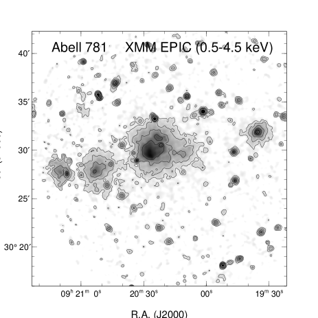
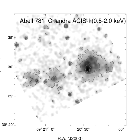
We were awarded 15ks of XMM-Newton time in cycle 2 to get a closer look at our top-ranked DLS cluster complex. This observation took place on 04 April 2003 (Obsid 0150620201). In addition, Chandra had observed A781 on 03 October 2000 with the ACIS-I detector for a nominal exposure time of 10 ks (Obsid # 534). The XMM-Newton and Chandra observations revealed that the A781 cluster complex consists of a large main cluster connected to a subcluster with two smaller clusters to its east and one to its west. We shall call the largest cluster the ‘Main’ cluster. The subcluster to its southwest appears in the act of merging with it (see Figure 1). Just to the east of the Main cluster is another cluster, which we will refer to as the ‘Middle’ cluster, and within the same pointing, further to the east, is another cluster, hereafter ‘East’ cluster. The XMM-Newton observation also presented us with a surprise. To the west of the Main cluster there appears to be one more cluster, which we will call the ‘West’ cluster. This cluster did not appear in the original DLS convergence maps made for the survey, and it is also, unfortunately, out of the field of view of the Chandra archive observations. Table 1 lists the IAU designations of these clusters.
| IAU Designation | Nickname |
|---|---|
| CXOU J092026+302938 | Main Cluster |
| CXOU J092053+302800 | Middle Cluster |
| CXOU J092110+302751 | East Cluster |
| CXOU J092011+302954 | Subcluster |
| XMMU J091935+303155 | West Cluster |
3.3. Optical Spectroscopy
Geller et al. (2005) conducted a magnitude-limited (to ) spectroscopic survey in this field. They report mean redshifts of 0.302, 0.291, and 0.427 for the Main, Middle, and East clusters respectively (labeled as clusters A, B, and C in Geller et al. (2005)). These redshifts were obtained from 163, 123, and 33 cluster members respectively. No redshift errors are quoted, however given the number of cluster members and the redshift errors in the individual galaxies, the systemic redshifts of the systems should be accurate to dz of 0.0002. The rest frame line-of-sight velocity dispersions were found to be km s-1 (Main), km s-1 (Middle), and km s-1 (East) (Geller et al., 2005). According to these velocity dispersions, these cluster components appear to be similar, a result we examine further using our X-ray and weak-lensing data.
The redshift of the West cluster is not reported in Geller et al. (2005). We obtained spectroscopy of this cluster with Keck/LRIS (Oke et al., 1995) in longslit mode on 16 January 2007. We obtained secure redshifts for two member galaxies, at a mean redshift of , though clearly the quoted error is itself highly uncertain with only two members. We also observed the East cluster in longslit mode on the same night, finding a mean redshift of based on two members, in agreement with Geller et al. (2005). Thus the East and West clusters are the only two components at the same redshift, but with a transverse separation of 21′ or 7.0 Mpc. Throughout this work we assume a CDM cosmology of , , and (Spergel et al., 2003).
4. Extracted X-ray Temperatures and Gas Density Profiles
To obtain X-ray mass estimates of these clusters, we follow the standard practice of treating the intracluster gas as a hydrostatic fluid. This assumption is reasonable for dynamically relaxed clusters since collision times for ions and electrons in the hot gas are very short compared to times scales over which the gas heats or cools or the cluster gravitational potential varies. Assuming spherical symmetry,
| (1) |
where is the gas mean molecular weight, and are the gas temperature and density profiles, and is the total mass within a radius . We assume the cluster gas follows a -model,
| (2) |
proposed by Cavaliere & Fusco-Femiano (1978). In this model, the core radius, , is where the density is half the central density for a typical of 2/3. To determine and , we note that the X-ray emissivity is proportional to the square of the cluster gas density times the cooling function, i.e., . Integrating the emissivity through the cluster line of sight gives the X-ray surface brightness . Assuming a -model for the gas density and noting that the cooling function is close to constant over the range of typical cluster temperatures yields
| (3) |
where and is the projected radius (e.g., Sarazin (1986)). We fit the radial X-ray surface brightness profile with equation 3 to obtain estimates for and (see §4.2).
The statistical quality of our data precludes the determination of a radial temperature profile. In lieu of this, we assume an NFW profile for the cluster matter density given by
| (4) |
where is the central density and is the scale radius (Navarro et al., 1996, 1997). This gives
| (5) |
for the mass within a radius r. Using equation 1, we solve for the cluster temperature profile and then for the emission-weighted, projected, average temperature within a given aperture, which our data allow us to measure relatively precisely. We compare this predicted temperature to our measured temperature determined from X-ray spectroscopy to find the best-fit value for and thus the cluster mass. We describe the details of the X-ray spectroscopy below.
| Chandra | source | background annulus (same center as source) |
|---|---|---|
| Main Cluster | 09:20:24.8 +30:30:20.4 2.4’ | 3.3’ – 4.3’ (minus Subcluster) |
| Middle Cluster | 09:20:52.5 +30:28:08.4 1.6’ | 2.3’ – 3.3’ (minus East) |
| East Cluster | 09:21:10.9 +30:28:04.2 1.5’ | 2.0’ – 3.0’ (minus Middle) |
| Subcluster | 09:20:09.4 +30:30:02.5 0.9’ | … |
| R.A. | Decl. | Radius |
|---|---|---|
| 09:20:32.590 | +30:29:10.49 | 4” |
| 09:20:29.774 | +30:28:55.73 | 2” |
| 09:20:59.852 | +30:27:29.23 | 8” |
| 09:20:50.765 | +30:29:22.97 | 5” |
| 09:20:45.587 | +30:28:39.22 | 8” |
| 09:21:06.817 | +30:27:40.20 | 11” |
| 09:21:05.684 | +30:29:02.13 | 6” |
| XMM-Newton | region |
|---|---|
| Main Cluster | 09:20:24.439 +30:30:21.12 2.5’ |
| Middle Cluster | 09:20:52.433 +30:28:12.74 1.4’ |
| East Cluster | 09:21:09.912 +30:27:58.31 1.1’ |
| Subcluster | 09:20:10.046 +30:29:57.17 1’ |
| West | 09:19:34.752 +30:32:00.88 1’ |
| Background Annulus | 09:20:12.521 +30:29:10.37 10.7’ – 13.7’ (minus East) |
| R.A. | Decl. | Radius |
|---|---|---|
| 09:20:33.209 | +30:28:58.48 | 17” |
| 09:20:24.600 | +30:33:19.12 | 24” |
| 09:20:21.809 | +30:30:35.14 | 16” |
| 09:20:34.805 | +30:29:47.02 | 12” |
| 09:20:25.531 | +30:33:39.11 | 12” |
| 09:20:45.588 | +30:28:39.22 | 12” |
| 09:21:06.816 | +30:27:40.20 | 11” |
4.1. X-ray Temperatures
4.1.1 Analysis of Chandra Data
We downloaded the Chandra data from the archive and used CIAO software tools for the initial data reduction steps. The observation was carried out in full-frame timed exposure mode using very faint telemetry mode. The peak X-ray emission of the Main cluster was positioned near the center of chip I3, some 3.5′ from the on-axis “sweet” spot of the high resolution mirror. The merging subcluster to the west was imaged on chip I3, while the two other clusters toward the east were imaged on chip I1. There was no cluster X-ray emission visible on the remaining two chips of the imaging array. We note that chip S2 of the spectroscopic array was also active during this observation, but we did not utilize these data. Event pulse heights were corrected for time-dependent gain, and all grades, other than 0, 2, 3, 4, and 6, were rejected. Information contained in the very faint mode data was used to reject non–X-ray background events. The light curve of the entire imaging array (minus obvious cluster and unresolved emission) was examined and no time intervals of high or excessive background were found. The resulting live-time corrected exposure time was roughly 9900 sec. Figure 1 shows the 500-2000 eV band image of the ACIS-I data after exposure correction (for which the vignetting function was calculated at a monochromatic X-ray energy of 1 keV) and smoothing with a Gaussian of .
Spectral extraction regions for the clusters were determined (see Tables 2 and 3) to optimize the signal to noise ratio of the resulting spectra. Annular regions surrounding each cluster were used to generate background spectra. Obvious point sources were excluded from both source and background regions, and cluster emission was excluded from all background regions. Weighted spectral response functions were generated for each source and matching background region, including instrumental absorption due to contamination build-up on the ACIS filters.
Xspec (version 11.3) was used for the spectral analysis. Fits were first done to the background spectra using a phenomenological model consisting of a non-X-ray background component (three gaussian lines and a power law to account for instrumental fluorescence lines and charged particles) and an astrophysical component (an absorbed power-law model to account for the unresolved X-ray background). Inclusion of a soft thermal component (from nearby diffuse Galactic emission, for example) did not significantly improve the background fits, so it was not included. The absorption column density was fixed to a value of atoms cm-2 based on Galactic HI measurements in this direction (Dickey & Lockman, 1990) and the photon index of the astrophysical background component was fixed to . Only the normalization of this power-law model was allowed to vary. For the non-X-ray background, the gaussian line centroids and normalizations as well as the power-law index and normalization were allowed to vary freely. There were a total of nine free parameters for the fits to the background spectra. The source spectra included a redshifted thermal plasma model (mekal, in xspec parlance) to account for the cluster emission as well as the full component of background models just described. In all cases best fits were determined using the “c-stat” fit statistic, which is a likelihood figure of merit function appropriate for Poisson-distributed data.
Each pair of matched source and background spectra was fitted jointly with the background spectral components scaled between the source and background based on the ratio of exposure integrated over the extraction regions. In the joint fits the normalizations of the two background power laws plus the non-X-ray background photon index were allowed to vary. The other background model parameter values were held fixed at values determined from the background fits alone.
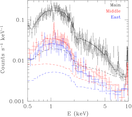
The best-fit temperature values and 1- statistical uncertainties are given in Table 6. For the East and Middle clusters, the metal abundance was held fixed to 0.3 times solar. For the Main cluster, because of its higher statistical level, this was allowed to vary yielding a best fit value of times solar (1- error). Redshifts were fixed to the values mentioned above. Figure 2 shows the best-fit spectra for these three clusters, where the dashed line represents the contribution from the background.
4.1.2 Analysis of XMM-Newton Data
The initial data reduction steps for the XMM-Newton data were completed using the SAS software tools. The data consists of observations from the three EPIC instruments, MOS1, MOS2, and PN. To model the non-X-ray background from charged particles and instrumental fluorescence lines, we also obtained closed observations (observations with the filter wheel in the closed position) for each of the three EPIC instruments. Thus we were able to use an independent measure of the particle background, differing from our Chandra analysis.
Both our cluster data and the closed data were filtered by pattern and energy range. We kept single and double pixel events and events with pulse heights in the range of 300 to 12000 eV for MOS observations. For PN observations, we only kept single pixel events and events with pulse heights between 300 and 15000 eV. We also chose the most conservative screening criteria (excluding events next to edges of CCDs and next to bad pixels, etc.). Our cluster and closed EPIC data were also filtered for soft solar proton flares.
Figure 1 shows the 500-4500 ev band image of the EPIC data after exposure correction and smoothing with a Gaussian of . Extraction regions for the clusters and point sources were identified along with a background annulus surrounding and away from any of the cluster regions (see Tables 4 and 5). Spectra were created of the cluster regions and background annulus for both the closed and cluster data, as were spectral response and effective area files. Resolved point sources were excluded from both the source and background regions, and cluster emission was also excluded from the background region.
Xspec was used to fit the spectra of the background annuli in the closed and cluster data using a similar phenomenological model as described for the Chandra analysis. The closed data background annulus was fit with several gaussians and three power laws to model the non-X-ray background. This best-fit model was used as a starting model to fit the spectrum of the cluster data background annulus, adding an absorbed power-law to model the unresolved X-ray background and an absorbed soft thermal (mekal) component to model the soft diffuse Galactic emission. The absorption column density and photon index of the astrophysical background model were fixed as mentioned above for the Chandra analysis, and the thermal component was given a fixed plasma temperature of 0.2 keV and a solar metal abundance. We linked the power-law norms of the particle background by the ratio of the power-law norms in the closed background data. This kept the slope and shape of the continuum fixed, but allowed the overall normalization to vary. The spectrum of the cluster data background annulus was fit by allowing the normalizations of the astrophysical background power-law and thermal component to vary as well as the normalization of the non-X-ray particle background.
A best-fit joint model was created to fit the background annulus spectra for the three instruments simultaneously. The parameters of the astrophysical background model were kept in common between the instruments, but the parameters of the particle background differed. A second thermal component was added to the astrophysical background model to better fit the spectra at energies below the aluminum fluorescence line. The normalizations, temperatures, and abundances of the two thermal components were allowed to vary as well as the unresolved X-ray background power law.
The source regions were fit drawing on the closed observations to fit the non-X-ray background and the annulus spectra to fit the astrophysical background. The spectra of the cluster regions in the closed observations were fit using the closed background annulus best-fit model as a starting point. The spectra of the source regions in our data were fit using models starting where the particle background normalization and the normalization of the strongest fluorescence line of each cluster region were set equal to those from the corresponding closed cluster region, scaled by the ratio of the normalizations between the observed and closed background annulus. The normalizations of the weaker fluorescence lines were set equal to the normalization of the strongest line scaled by the ratio of the weak-line norm to the strong-line norm in the corresponding closed cluster region. The astrophysical background model was taken from the best joint-fit model for the background annulus, where the normalizations of the background spectral components were scaled by the ratio of the exposure integrated over the source and background regions. The source spectra were modeled with a redshifted mekal thermal plasma model, with the abundance equal to 0.3 times solar and the temperature and normalization allowed to be free parameters.
We fit the spectra of the source regions using these starting models by first fitting the normalization of the particle background using only events greater than 10 keV, with the cluster model zeroed out. With this normalization frozen, we fit the temperature and norm of the cluster model using only events below 10 keV. The particle background norm was then refit using events larger than 10 keV and this frozen cluster model.
Having fit for the particle background of each source region for each instrument, the best-fit source models for the three instruments were combined to allow for a joint fit. Again for the joint fit, the astrophysical background model was kept the same for each instrument except that the normalizations differed due to different exposure scalings. This fit was done using the best-fit particle background normalizations described above and those differing by 1- for each instrument. In this way, we were able to model the systematic uncertainties arising from the particle background subtraction.
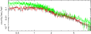
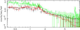
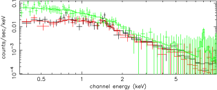
The 1- errors on the cluster temperature were obtained using a delta fit statistic of 1.0 for the one interesting parameter. The resulting best-fit temperatures and error bars are given in Table 6. We find good agreement between the Chandra and XMM-Newton best-fit temperatures given the statistical and systematic uncertainties. The XMM-Newton spectra for the four main clusters and the best joint-fit models are shown in Figures 3 and 4.

4.2. X-ray Surface Brightness Profiles
A surface brightness profile was created by first determining the surface brightness peak of each cluster. This was done with exposure corrected images in the 500-2000 eV band for each instrument smoothed with a Gaussian of . The vignetting function for the exposure maps was calculated at the monochromatic X-ray energy of 1.25 keV for XMM-Newton and 1 keV for Chandra.
The unsmoothed images and exposure maps from the three EPIC instruments and Chandra were used to generate surface brightness profiles. Images and exposure maps from the separate EPIC focal plane detectors were summed to create a joint XMM image and corresponding exposure map. Exposure maps in all cases were made including the effective area, for proper weighting of the XMM detectors and for ease of comparing the XMM and Chandra profiles.
We chose 40 radial bins of 8′′ each, centered around the surface brightness peak of each cluster to find profiles that extend out to 5.3’. In each radial bin, we summed the counts from the Chandra/joint XMM image and divided this sum by the total exposure in that bin from the corresponding exposure map. We calculated the error on the surface brightness in each radial bin by using the small count statistic (Gehrels, 1986), where units of exposure are given in sec cm2 arcmin2.
Using the radial bins farthest from the surface brightness peaks, we inferred the surface brightness due to the background. We then fit the surface brightness profiles to equation 3 by fixing the background and allowing , , and the overall normalization to vary as free parameters. The profiles and best-fit models are displayed in Figures 5 and 6. Table 7 gives the and best-fit values for each cluster along with their 1- statistical error bars. There is good agreement between the Chandra and XMM-Newton best-fit and values given the statistical uncertainties.


| Cluster | XMM counts | XMM kT (keV) | Chandra counts | Chandra kT (keV) |
|---|---|---|---|---|
| East Cluster | 505 | 300 | ||
| Middle Cluster | 1135 | 380 | ||
| Main Cluster | 8812 | 2400 | ||
| West Cluster | 1163 | 0 | … |
| Cluster | XMM | XMM (arcmin) | Chandra | Chandra (arcmin) |
|---|---|---|---|---|
| East Cluster | ||||
| Middle Cluster | ||||
| Main Cluster | ||||
| West Cluster | … | … |
| Cluster | XMM | XMM | Chandra | Chandra |
|---|---|---|---|---|
| (Mpc) | () | (Mpc) | () | |
| East Cluster | 0.91 | 2.5 | 0.99 | 3.2 |
| Middle Cluster | 0.84 | 1.7 | 1.01 | 3.0 |
| Main Cluster | 1.38 | 7.6 | 1.48 | 9.5 |
| West Cluster | 0.89 | 2.4 | … | … |
5. Mass Estimates
5.1. X-ray Masses
To determine each cluster’s X-ray derived mass, we use equations 1, 2, and 5 and our best-fit and values to predict the cluster temperature profile for given values of the central density and scale radius in the NFW profile. The solution of the temperature profile requires a boundary condition. We assume the cluster temperature to be 1.25 keV at 3.5 Mpc for each cluster but allow this outer temperature and radius to vary generously over the range of 0.5 to 2 keV and 2 to 5 Mpc and fold this uncertainty into our error bars. We find that this variation in our boundary conditions contributes a negligible amount (less than ) to our error estimates.
To compare each cluster’s X-ray and weak-lensing-derived masses in an mutually consistent manner, we must assume the same matter density profile for each method. Since neither the X-ray nor the weak-lensing data is deep enough to well constrain both and in the NFW profile, we choose to estimate each cluster’s concentration parameter, , using results from hydrodynamic simulations and an X-ray estimate of each cluster’s mass assuming isothermality. This mass estimate is accurate enough to give a reasonable estimate of the concentration parameter since the concentration is a slowly varying function of cluster mass. The concentration parameter is here defined as , where is the radius within which the cluster mean density is 500 times the critical density. We again use the isothermal case to estimate , which yields an estimate of . Since we are primarily interested in the comparison between X-ray-derived and weak-lensing-derived masses, the accuracy of the scale radius is less important than the fact that we used the same scale radius in deriving the masses using both methods. A change in the scale radius may introduce a systematic shift in the masses but will not alter significantly their ratio.
5.1.1 Masses Assuming an Isothermal- Model
We determine X-ray isothermal -model mass estimates for these clusters as an intermediate step to estimate the NFW scale radius for each cluster. If we assume that each cluster is isothermal with a gas density given by equation 2, then equation 1 can be rewritten to give
| (6) | |||||
where we set for the cluster gas (Evrard et al., 1996). Using the best-fit , , and for each cluster from Chandra and XMM-Newton observations, we calculate for each cluster, which is the mass within . The best-fit and for each cluster from each X-ray satellite are listed in Table 8. This table is without error bars since we only use these values to estimate a reasonable for each cluster.
We use the above XMM and values and predictions for the concentration as a function of mass and redshift derived from hydrodynamic cluster simulations (Dolag et al., 2004) to obtain an estimate of . The relation used here is from the Dolag et al. (2004) CDM cosmological simulation, and we converted our masses and radii to the definitions used in that work to determine . This concentration relation has a reasonable agreement with Chandra observations of nearby clusters (Vikhlinin et al., 2006). We choose to use XMM -model masses since we have XMM observations for all four clusters. Table 9 lists the best estimates of . We hold this scale radius fixed and keep it in common when deriving masses from weak-lensing and X-ray methods and focus on the relative difference in mass estimates using these two methods.
5.1.2 Masses Assuming an NFW Profile
Given an estimate of , , and for each cluster, we vary and calculate the emission-weighted, projected, average temperature within an aperture (as discussed in §4). The apertures for each cluster and instrument are given in Tables 2 and 4. We match the predicted temperatures to our measured temperatures in Table 6 to find the best-fit central densities. The 1- errors on are calculated by varying the measured , , and parameters within their 1- error bars and treating and as correlated variables. The variation in the boundary condition introduces a negligible error on as mentioned above. Best-fit measurements and 1- errors for Chandra and XMM observations are given in Table 9. There is good agreement between the two instruments, and we calculate a weighted average to give a combined X-ray for each cluster, which we also list in Table 9. Given and , X-ray masses are calculated using equation 5 and listed in Table 10. These masses are calculated using the combined X-ray for all the clusters except the West cluster, for which only the XMM is available.
5.2. Weak-Lensing Masses
The weak lensing mass estimates are based on the full DLS exposure time of 18 ks in and 12 ks in , rather than the partially complete imaging used for cluster discovery in Wittman et al. (2006). Otherwise, image processing was as described in detail in that paper. The data were taken in good seeing conditions (FWHM ) and are used to measure the galaxy shapes. The A781 complex spans two contiguous DLS “subfields” or pointing centers. The FWHM of the final images, after circularizing the PSF and co-adding 20 exposures, is and for the two subfields involved. The data are used only to provide color information for photometric redshifts.
We extracted shear catalogs using a partial implementation of Bernstein & Jarvis (2002). This implementation appeared as the “VM” method in Heymans et al. (2006), which compared different weak-lensing methods on a set of simulated sheared images. After correcting for stellar contamination which was present in that dataset but not here, the VM method yielded 89% of the true shear in those images. In this work, we divide the VM results by 0.89 to more closely approximate the true shear. However, we recognize that this correction factor is likely to be data-dependent, and we therefore assign a systematic error of 10% to the shear calibration.
We derived photometric redshifts using BPZ (Benítez, 2000) with the HDF prior. We optimized the templates using a subset of the SHELS (Geller et al., 2005) spectroscopic sample and the procedure of Ilbert et al. (2006). Complete details are discussed elsewhere (Margoniner et al., in preparation). To assess the accuracy of these photometric redshifts, we turn to an independent spectroscopic sample, consisting of all redshifts in DLS field F2 in the literature, as tabulated by the NASA/IPAC Extragalactic Database. We find 328 galaxies with spectroscopic redshifts that match our cleaned photometry (unsaturated, not near bright stars, etc), spanning the redshift range 0.02—0.70. The resulting rms photometric redshift error per galaxy is , with a bias of , and no catastrophic outliers.
Because shear is nonlocal and mass maps tend to be highly smoothed, the presence of one clump may affect the apparent mass density of another clump. This is true of the Wittman et al. (2006) maps, and we eliminate that effect here by simultaneously fitting axisymmetric NFW profiles to the four X-ray positions. The model fitting takes into account the full three-dimensional position (RA, DEC, z) of each source galaxy. The per-galaxy imprecision in is not important because the lensing kernel is very broad, and because each galaxy is a very noisy estimator of the shear: a 0.1 shift in source redshift changes the modeled shear by much less than the per-galaxy shear error. For each NFW model, RA and DEC were fixed by the X-ray position, was fixed by the spectroscopy, and was fixed to the value used for the X-ray fitting. Thus only one parameter, , was fit for each model. Wright & Brainerd (2000) give expressions for shear induced by an NFW profile.
Of the 350,000 galaxies in the 22∘ DLS field containing A781, we limited the fit to galaxies within 15′ of a clump center, for computational efficiency and because more distant galaxies may be influenced more by other clusters than by those in the A781 complex. We also cut on photometric redshift, because cluster members scattering to higher redshift would reduce the estimated shear (slightly, because of their low inferred distance ratio), while cluster members scattering to lower redshift would have no effect. We did fits with cuts at (just behind the richer, lower-redshift clumps) and ( beyond the higher-redshift clumps), and found a difference of in the fitted parameters. The lenient (strict) cut yielded 30137 (22173) galaxies, or 23 (17) arcmin-2 over 1320 arcmin2, although 10% of this area was masked due to bright stars. We adopt the strict cut to avoid any question of contamination. The resulting source catalogs show no increased density near the clump centers.
Because shear from an NFW profile is linear in , we used singular value decomposition (SVD) as described in Press et al. (1992)). This solves the general linear least squares problem in one pass, with no iteration required. The galaxies were given equal weights in the fit, because the VM shear method does not assign weights to galaxies. However, the importance of a galaxy in determining the fit still depends on its position and redshift, through the model’s dependence on position and redshift. We then corrected for the fact that the observable in weak lensing is not the shear , but the reduced shear (where is the convergence) as follows. We computed the convergence of the best-fit model at the location of each source galaxy, constructed a reduced-shear model, redid the linear fit, and iterated. In the first iteration, this resulted in a 5% correction to the fit parameters. In the second iteration, the correction was only 0.2%, much smaller than the fitted parameter statistical uncertainties, and therefore the reduced-shear fit was deemed to have converged.
The fitted ’s and their uncertainties are listed in Table 9. The uncertainties output by the SVD routine were confirmed by 1000 bootstrap resampling realizations. Although the fit is not -driven, we can define a statistic to see how much of the variance in the data is explained by the model. There are 44326 degrees of freedom because each galaxy has two shear components. For each component of shear, we compute the rms without any fit and define that as the uncertainty associated with each galaxy. This results in an initial of 44326, which is decreased by 40.4 when the four-parameter model is subtracted off. The chance of this happening randomly is for Gaussian distributions. The remaining variance is due mostly to the intrinsically random distribution of galaxy shapes (shape noise) and shape measurement errors, although a small amount may be attributed to additional structure in the field as indicated by the following mass maps.
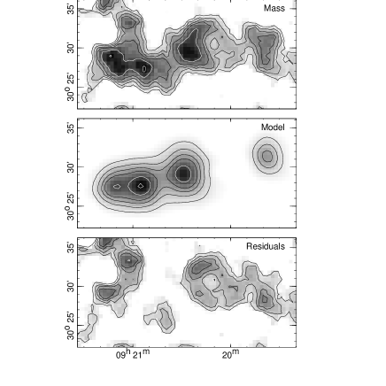
We show the fit visually in Figure 7. The top panel shows a mass map made using the method described in Wittman et al. (2006) (originally from Fischer & Tyson (1997)), the middle panel shows a similar map made from the model shears, and the bottom panel shows a map made from the residual shear after subtracting off the fit. The Main, Middle, and East clumps have been mostly subtracted, but the West clump has not been well modeled. There is also an unmodeled mass clump just northwest of the East clump (RA 9:21, Dec 30:33), which appears to have some associated galaxies. We caution that the mass map is a sanity check rather than a quantitative indicator of goodness-of-fit, because it does not fold in source redshift information.
| Cluster | Estimated | XMM | Chandra | Combined X-ray | DLS |
|---|---|---|---|---|---|
| (Mpc) | ( g/cm3) | ( g/cm3) | ( g/cm3) | ( g/cm3) | |
| East | 0.37 | ||||
| Middle | 0.31 | ||||
| Main | 0.60 | ||||
| West | 0.33 | … |
| Cluster | X-ray | X-ray | Weak-lensing | Weak-lensing |
|---|---|---|---|---|
| (Mpc) | () | (Mpc) | () | |
| East Cluster | ||||
| Middle Cluster | ||||
| Main Cluster | ||||
| West Cluster |
In Table 9, weak-lensing errors are of two types, the first is statistical and the second is systematic. For the statistical errors, we performed bootstrap resampling to estimate the covariance of the cluster mass estimates. The masses of neighboring clusters (in projection) are anticorrelated, because the observed shear in a region must include the sum of the model shears from the neighbors. The errors given here for each cluster are after marginalizing over the allowed values for the other clusters. Therefore, the error on the total mass of all the clusters would be smaller than the quadrature sum of the errors given here. Also, the covariance will affect the comparison of the lensing for one of the four clusters to that for any of the others.
Systematic errors include shear calibration, source redshift calibration, mass sheet degeneracy, and residual cluster member contamination. We assign a shear calibration systematic uncertainty of 10% as explained above. We explored the effects of source redshift errors by fitting to different source redshift ranges. We find that only if we include photometric redshifts beyond 1.4, where the 4000 Å break redshifts out of the z′ filter, do the results change by as much as 10%. Even in that case, the results appear to change randomly rather than systematically, with some clumps increasing in fitted mass and others decreasing. Given these results, and the small bias in photometric redshifts when compared to the spectroscopic sample from the literature, a systematic error of 5% in mass due to redshift calibration errors is very conservative.
We estimate residual cluster member contamination by examining the source galaxy areal density around the richest (Main) clump. There is an excess in the central 2′ radius. Comparing the redshift distribution in that area to a control annulus, we find 58 excess galaxies at redshifts 0.35–0.42, presumably cluster members with photometric redshift errors. In the fit, all galaxies were weighted equally, so their relative importance is determined by their proximity (in three dimensions) to where the model reduced shear is large. These galaxies are near the projected center of the lens, but at low inferred distance ratio. We compute their effective weight as the square of the model reduced shear, and compare their total weight to the rest of the galaxies within 5′ of the Main clump. The summed weight of the interloping galaxies is only 0.010 times that of the valid source galaxies, which presumably resulted in a 1% underestimate of the mass, much smaller than the other systematics.
The last systematic involves mass sheet degeneracy and projection of unrelated structures near the line of sight. If our assumption of an NFW profile is correct, then mass sheet degeneracy is not an issue, because we are fitting the profile rather than empirically determining departures from a baseline. Measuring shear to as large a radius as possible would help check the profile assumption, just as it would help reduce mass sheet degeneracy. However, going to large radii increases the chance of including some unrelated structure projected near the line of sight. Metzler et al. (2001) (hereafter M01) characterized this by measuring lensing masses of clusters in large-scale numerical simulations as a function of data set radius. The truncation radius used in the fitting here, 30′, corresponds to a transverse separation of about 5 Mpc, for which M01 find a scatter of about 7%. (Note that M01’s systematic offset in the population is not relevant here because profile fitting is less biased than their aperture densitometry.) Scatter in the population becomes a systematic when considering a single cluster. However, by simultaneously fitting multiple clumps, this systematic is probably already greatly reduced. We empirically test this effect by varying the truncation radius and find that the results can change by up to 5%. We therefore assign a systematic of 5% due to this effect. The larger systematic is likely to be in the profile assumption. This systematic is likely to be on the same order as the mass sheet degeneracy systematic incurred if the profile assumption were dropped, which is quoted as by Bradač et al. (2004).
In summary, the systematics include for the profile assumption and/or mass sheet degeneracy, for shear calibration, for projections, and for photometric redshift errors. We include only the latter three systematic errors in Table 9, where we assume an NFW profile accurately describes the matter density. This allows us to compare the X-ray and weak-lensing values. In table 10, we present a summary of the and values, where the the weak-lensing statistical and systematic error bars on are added in quadrature. It should be kept in mind that the absolute masses of the clusters depend on the profile assumption.
6. DISCUSSION
Comparison of the X-ray and weak-lensing values indicates that these values are in agreement for the East, Middle, and West clusters. This agreement suggests that line-of-sight mass contributions have not significantly biased the weak-lensing measurements.
For the Main cluster, the X-ray-derived is higher than that from weak-lensing by about 2. The X-ray images of the Main cluster suggest it may be undergoing a merger with a subcluster (see Figure 1), and thus may be out of hydrostatic equilibrium. From the literature it is not obvious whether cluster mergers are expected to bias X-ray mass estimates high or low. Weak-lensing observations of 22 X-ray bright clusters at found X-ray temperatures higher by than those inferred from weak-lensing, for clusters with keV (Cypriano et al., 2004). The largest discrepancy in this sample was for the two clusters with the highest X-ray temperatures ( keV), which both show signs of being out of dynamical equilibrium. It is a reasonable extrapolation to presume that all the clusters with keV in their sample are unrelaxed, with the temperature of their intracluster medium boosted by shocks due to in-falling groups and mergers with other clusters.
However, recent hydrodynamic simulations indicate that unrelaxed cluster temperatures should be lower than those for relaxed clusters of the same mass (Kravtsov et al., 2006; Nagai et al., 2007). The reasoning for this is that over the course of a merger, the mass of the system increases faster than the conversion of the kinetic energy of the merging systems into thermal energy of the intracluster medium (Kravtsov et al., 2006). It has also been suggested from hydrodynamic simulations of merging clusters that X-ray mass estimates based on hydrostatic equilibrium can be biased high close to core-crossing, where a temperature boost occurs due to shocks, but can be biased low just before and after this temperature spike (Poole et al., 2006; Puchwein & Bartelmann, 2007). This latter scenario is possibly supported by recent X-ray and weak-lensing observations of 10 X-ray luminous clusters at (Zhang et al., 2007; Bardeau et al., 2007). The X-ray observations of this sample were carried out with XMM-Newton, and the weak-lensing is from ground-based imaging with the CFH12k camera on CFHT. These authors report that four out of these ten clusters have consistent X-ray and weak-lensing mass estimates. Of the six clusters that show a mass discrepancy, half have higher and half have lower X-ray as compared to weak-lensing masses.
It is possible that the Main cluster in the A781 cluster complex is close to core-crossing as our X-ray mass estimate is biased high. It is also possible that a selection effect is occurring in the sample of Cypriano et al. (2004) where the clusters with keV are in a state of high temperature boosting and thus close to core-crossing. Deeper X-ray observations of this A781 cluster and further comparisons of weak-lensing and X-ray mass estimates of known merging clusters will help to clarify the biases expected from dynamically unrelaxed systems.
The West cluster did not appear in our original shear maps, and we confirm here that it is a low significance weak-lensing detection (1-2). It was detected in the X-ray by chance as it fell within the same XMM-Newton pointing as the other three clusters. However, weak-lensing and X-ray data yield consistent mass estimates. We measure a very small core radius for this cluster (), consistent with most of the emission coming from a compact core. Northwest of the East cluster, we also find an enhancement in both the galaxy distribution and lensing signal, and we find some indication of X-ray emission from that region. Further X-ray observations would allow us to study these lower mass systems in more detail.
Based on the limited information available, the velocity dispersion values appear broadly consistent with the East, Middle, and Main clusters having nearly equal masses (Geller et al., 2005). This agrees with the similarity in weak-lensing masses we present here (see Table 10). A detailed comparison of the cluster masses derived above with the velocity distributions is beyond the scope of this work. Study of the velocity distribution of the potentially merging component (Main cluster) could shed light on the epoch and geometry of the merger (see Gómez et al. (2000)).
7. CONCLUSION
Many cluster surveys will take place over the next few years at several different wavebands. Already considerable samples of X-ray and optically selected clusters have been compiled. In addition, sizeable microwave and shear-selected samples are close at hand. These surveys can probe with precision the growth of structure over cosmic time, and thereby open a new window on cosmology. However, the two main hurdles to overcome are relating cluster observables to mass and characterizing the sample selection. By comparing weak-lensing and X-ray observations and mass estimates for clusters in the DLS shear-selected sample we hope to understand the systematic biases in both mass estimation methods and modes of cluster selection.
An analysis of the top shear-ranked mass distribution in the DLS sample reveals a complex of four clusters, the largest of which can be identified as A781. The four clusters are at distinctly different redshifts, as determined by optical spectroscopy, and the X-ray images suggest three are dynamically relaxed while the largest cluster appears to be merging with a small subcluster. Masses from both X-ray and weak-lensing observations were determined assuming an NFW profile for the matter density. Since neither sets of observations were deep enough to well constrain both the central density and scale radius of each cluster NFW profile, we estimated the scale radii using X-ray-derived isothermal -model mass estimates and a relation describing concentration as a function of mass and redshift derived from cosmological hydrodynamic simulations. For each cluster profile, the same scale radius was used to determine the best-fit X-ray and weak-lensing central densities. We focus on the difference in central densities derived with each method as the central density scales linearly with mass.
We find that three out of the four clusters show agreement between their X-ray and weak-lensing derived central densities. The fourth and largest cluster has an X-ray derived central density higher than that derived from weak-lensing by about 2. This discrepancy is most likely due to the cluster’s disrupted dynamical state. Recent weak-lensing observations of X-ray selected clusters and hydrodynamic simulations leave some ambiguity about whether dynamical disruption via cluster mergers biases X-ray mass estimates high or low. The direction of the bias may be related to the stage of the merger, e.g., whether it is close to core-crossing or more advanced. Deeper X-ray observations of this cluster to better resolve the merger and further comparisons between weak-lensing and X-ray-derived masses of known merging clusters will shed greater light on this issue.
Initial steps are being made by many groups to overcome the above mentioned hurdles regarding the use of clusters as precision tracers of structure growth. Our collaboration, for example, has Chandra and XMM-Newton data on a larger sample of DLS shear-selected clusters that we will be reporting on in future publications. Hopefully all these efforts will open a new window through which we can understand our universe.
References
- Bardeau et al. (2007) Bardeau, S., Soucail, G., Kneib, J. P., Czoske, O., Ebeling, H., Hudelot, P., Smail, I., & Smith, G. P. 2007, A&A, 470, 449
- Benítez (2000) Benítez, N. 2000, ApJ, 536, 571
- Bernstein & Jarvis (2002) Bernstein, G. M., & Jarvis, M. 2002, AJ, 123, 583
- Bradač et al. (2004) Bradač, M., Lombardi, M., & Schneider, P. 2004, A&A, 424, 13
- Carlstrom et al. (2002) Carlstrom, J. E., Holder, G. P., & Reese, E. D. 2002, ARA&A, 40, 643
- Cavaliere & Fusco-Femiano (1978) Cavaliere, A., & Fusco-Femiano, R. 1978, A&A, 70, 677
- Cypriano et al. (2004) Cypriano, E. S., Sodré, L. J., Kneib, J.-P., & Campusano, L. E. 2004, ApJ, 613, 95
- Dahle et al. (2002) Dahle, H., Kaiser, N., Irgens, R. J., Lilje, P. B., & Maddox, S. J. 2002, ApJS, 139, 313
- de Putter & White (2005) de Putter, R., & White, M. 2005, New Astronomy, 10, 676
- Dickey & Lockman (1990) Dickey, J. M., & Lockman, F. J. 1990, ARA&A, 28, 215
- Dolag et al. (2004) Dolag, K., Bartelmann, M., Perrotta, F., Baccigalupi, C., Moscardini, L., Meneghetti, M., & Tormen, G. 2004, A&A, 416, 853
- Erben et al. (2000) Erben, T., van Waerbeke, L., Mellier, Y., Schneider, P., Cuillandre, J.-C., Castander, F. J., & Dantel-Fort, M. 2000, A&A, 355, 23
- Evrard et al. (1996) Evrard, A. E., Metzler, C. A., & Navarro, J. F. 1996, ApJ, 469, 494
- Fischer & Tyson (1997) Fischer, P., & Tyson, J. A. 1997, AJ, 114, 14
- Gavazzi & Soucail (2007) Gavazzi, R., & Soucail, G. 2007, A&A, 462, 459
- Gehrels (1986) Gehrels, N. 1986, ApJ, 303, 336
- Geller et al. (2005) Geller, M. J., Dell’Antonio, I. P., Kurtz, M. J., Ramella, M., Fabricant, D. G., Caldwell, N., Tyson, J. A., & Wittman, D. 2005, ApJ, 635, L125
- Gómez et al. (2000) Gómez, P. L., Hughes, J. P., & Birkinshaw, M. 2000, ApJ, 540, 726
- Gray et al. (2001) Gray, M. E., Ellis, R. S., Lewis, J. R., McMahon, R. G., & Firth, A. E. 2001, MNRAS, 325, 111
- Heymans et al. (2006) Heymans, C., et al. 2006, MNRAS, 368, 1323
- Hughes et al. (2004) Hughes, J. P., et al. 2004, in “Multiwavelength Cosmology”, Astrophysics and Space Science Library, Volume 301, ed. Manolis Plionis, p.255
- Ilbert et al. (2006) Ilbert, O., et al. 2006, A&A, 457, 841
- Koopmans et al. (2000) Koopmans, L. V. E., et al. 2000, A&A, 361, 815
- Kravtsov et al. (2006) Kravtsov, A. V., Vikhlinin, A., & Nagai, D. 2006, ApJ, 650, 128
- Margoniner & Wittman (2007) Margoniner, V., & Wittman, D. 2007, ApJ, submitted (arXiv:0707.2403)
- Metzler et al. (2001) Metzler, C. A., White, M., & Loken, C. 2001, ApJ, 547, 560
- Metzler et al. (1999) Metzler, C. A., White, M., Norman, M., & Loken, C. 1999, ApJ, 520, L9
- Miralles et al. (2002) Miralles, J.-M., et al. 2002, A&A, 388, 68
- Muller et al. (1998) Muller, G. P., Reed, R., Armandroff, T., Boroson, T. A., & Jacoby, G. H. 1998, in Proc. SPIE Vol. 3355, p. 577-585, Optical Astronomical Instrumentation, Sandro D’Odorico; Ed., 577
- Nagai et al. (2007) Nagai, D., Vikhlinin, A., & Kravtsov, A. V. 2007, ApJ, 655, 98
- Navarro et al. (1996) Navarro, J. F., Frenk, C. S., & White, S. D. M. 1996, ApJ, 462, 563
- Navarro et al. (1997) Navarro, J. F., Frenk, C. S., & White, S. D. M. 1997, ApJ, 490, 493
- Oke et al. (1995) Oke, J. B., Cohen, J. G., Carr, M., Cromer, J., Dingizian, A., Harris, F. H., Labrecque, S., Lucinio, R., Schaal, W., Epps, H., & Miller, J. 1995, PASP, 107, 375
- Poole et al. (2006) Poole, G. B., Fardal, M. A., Babul, A., McCarthy, I. G., Quinn, T., & Wadsley, J. 2006, MNRAS, 373, 881
- Press et al. (1992) Press, W. H., Teukolsky, S. A., Vetterling, W. T., & Flannery, B. P. 1992, Numerical Recipes in C (2nd ed.; Cambridge: Cambridge University Press)
- Puchwein & Bartelmann (2007) Puchwein, E., & Bartelmann, M. 2007, A&A, 474, 745
- Sarazin (1986) Sarazin, C. L. 1986, Reviews of Modern Physics, 58, 1
- Schirmer et al. (2007) Schirmer, M., Erben, T., Hetterscheidt, M., & Schneider, P. 2007, A&A, 462, 875
- Spergel et al. (2003) Spergel, D. N., et al. 2003, ApJS, 148, 175
- Umetsu & Futamase (2000) Umetsu, K., & Futamase, T. 2000, ApJ, 539, L5
- Vikhlinin et al. (2006) Vikhlinin, A., Kravtsov, A., Forman, W., Jones, C., Markevitch, M., Murray, S. S., & Van Speybroeck, L. 2006, ApJ, 640, 691
- Weinberg & Kamionkowski (2002) Weinberg, N. N., & Kamionkowski, M. 2002, MNRAS, 337, 1269
- White et al. (2002) White, M., van Waerbeke, L., & Mackey, J. 2002, ApJ, 575, 640
- Wittman et al. (2006) Wittman, D., Dell’Antonio, I. P., Hughes, J. P., Margoniner, V. E., Tyson, J. A., Cohen, J. G., & Norman, D. 2006, ApJ, 643, 128
- Wittman et al. (2003) Wittman, D., Margoniner, V. E., Tyson, J. A., Cohen, J. G., Becker, A. C., & Dell’Antonio, I. P. 2003, ApJ, 597, 218
- Wittman et al. (2001) Wittman, D., Tyson, J. A., Margoniner, V. E., Cohen, J. G., & Dell’Antonio, I. P. 2001, ApJ, 557, L89
- Wittman et al. (2002) Wittman, D. M., et al. 2002, in Survey and Other Telescope Technologies and Discoveries. Edited by Tyson, J. Anthony; Wolff, Sidney. Proceedings of the SPIE, Volume 4836, pp. 73-82 (2002)., 73
- Wright & Brainerd (2000) Wright, C. O., & Brainerd, T. G. 2000, ApJ, 534, 34
- Zhang et al. (2007) Zhang, Y.-Y., Finoguenov, A., Böhringer, H., Kneib, J.-P., Smith, G. P., Czoske, O., & Soucail, G. 2007, A&A, 467, 437