The light variability of the helium strong star HD 37776 as a result of its inhomogeneous elemental surface distribution

We simulate light curves of the helium strong chemically peculiar star HD 37776 assuming that the observed periodic light variations originate as a result of inhomogeneous horizontal distribution of chemical elements on the surface of a rotating star. We show that chemical peculiarity influences the monochromatic radiative flux, mainly due to bound-free processes. Using the model of the distribution of silicon and helium on HD 37776 surface, derived from spectroscopy, we calculate a photometric map of the surface and consequently the $uvby$ light curves of this star. Basically, the predicted light curves agree in shape and amplitude with the observed ones. We conclude that the basic properties of variability of this helium strong chemically peculiar star can be understood in terms of the model of spots with peculiar chemical composition.

1 Introduction

Periodic light variations are a common feature observed in the magnetic chemically peculiar (CP) stars. They can be interpreted by the presence of “photometric” spots causing an uneven distribution of the emergent flux on the surface of rotating stars. Likely, these hypothetical photometric spots are somehow related to the “spectroscopic” spots of a peculiar abundance of various chemical elements. Within this paradigm, the departures of the energy distribution in spectra of CP stars from the energy distribution of normal stars of the same spectral type are as a rule explained as a consequence of line blanketing by plenty of lines originating in the spectroscopic spots with peculiar chemical composition and the flux redistribution induced by them (Peterson 1970; Molnar 1973). Lanz et al. (1996) and Krtička et al. (2004) suggested that bound-free transitions may play a more important role in the blanketing, redistribution of the emergent flux, and the light variability.

However, more effects may influence the spectral energy distribution and consequently may be invoked to explain the observed light variability. These effects may be connected with the influence of complex surface magnetic fields. Staude (1972) and Trasco (1972) showed that the influence of the magnetic pressure on the stellar atmosphere structure might cause observable light variations (see also Stȩpień 1978; Carpenter 1985; LeBlanc et al. 1994). The effect of the magnetic field on the atmosphere hydrostatic equilibrium was recently studied by Valyavin et al. (2004). The influence of the Zeeman effect on the line blanketing may modify the emergent radiative flux (Kochukhov et al. 2005; Khan & Shulyak 2006). Consequently, there are many different mechanisms that might result in the appearance of photometric spots on the stellar surface.

Contrary to these photometric spots, the location and size (e.g., maps of distribution of individual chemical elements on the stellar surface) of the spectroscopic spots can be determined by Doppler imaging techniques (e.g., Khokhlova et al. 1997). However, it is not clear whether and how the photometric spots are related to the spectroscopic ones.

Another explanation of the light variability of hot stars with strong surface magnetic fields exists. Nakajima (1985) and Smith & Groote (2001) proposed that the observed light variations may be caused by light absorption in rotating circumstellar clouds. Recently, this model was successfully used by Townsend et al. (2005) for prediction of the light curve of the He-rich chemically peculiar star $σ$~Ori~E. The properties of these circumstellar clouds were inferred using the rigidly rotating magnetosphere model (Townsend & Owocki 2005), in which the material blown from the star by the radiatively driven wind accumulates in the potential minima along individual magnetic field lines. Townsend et al. (2005) used free parameters characterizing an amount of absorption in the clouds to predict the light curve of $\sigma$ Ori E, as it was not known for how long the accumulation had proceeded. Consequently, they were able to reproduce the shape of the light curve, but not the amplitude itself. Moreover, $\sigma$ Ori E shows hydrogen emission lines that indicate the presence of circumstellar environment. Last but not least, the light curve of $σ$~Ori~E is exceptional when compared with the light curves of other CP stars. However, many CP stars showing light variability are likely too cool to have sufficiently strong winds enabling formation of circumstellar clouds. Thus, the light variability of other CP stars may be caused by other mechanisms.

The fact that CP stars in many cases show not only peculiar chemical composition, but also a variable spectrum – indicating the uneven distribution of chemical elements on their surfaces – tempts one to attribute the light variability to this uneven surface distribution of elements. This uneven distribution, through the line blanketing and/or the bound-free absorption, determines the emergent flux depending on the location on the stellar surface and may cause the variability of a rotating star. However, to our knowledge, a light curve of a CP star had never been calculated ab initio from the known distribution of chemical elements as derived by Doppler imaging techniques. The initial step in this direction was done by Krivosheina et al. (1980), who were able to successfully reproduce the observed $vby$ light curve of CU Vir modifying the temperature gradient in the regions of silicon overabundance.

For our simulations of the light curves of chemically peculiar stars we selected HD 37776. This star residing in the reflection/emission nebula IC 431 (van den Bergh 1966; Finkbeiner 2003) belongs to well-studied helium-strong CP stars. It has a very strong complex surface magnetic field with a significant quadrupolar component (Borra & Landstreet 1979; Thompson & Landstreet 1985). The observed periodic variations of helium lines (Nissen 1976; Pedersen & Thomsen 1977) and lines of some lighter elements (Shore & Brown 1990) are interpreted as a consequence of rotation of a star with uneven elemental surface distribution. Based on this model, surface distributions and abundances of various elements were derived from spectroscopy (Bohlender & Landstreet 1988; Vetö et al. 1991; Khokhlova et al. 2000). Consequently, this star seemed to us to be an appealing target for modelling of the light variations.

In this work we present computed light curves of the He-strong CP star HD~37776. We used the surface distributions and abundances of various elements derived by Khokhlova et al. (2000). As silicon and helium create areas with large overabundances, and moreover, as it is known that silicon may influence the observed spectral energy distribution of silicon-rich CP stars (Artru & Lanz 1987; Lanz et al. 1996; Krtička et al. 2004), we concentrated on these two elements in our calculations. The role of silicon may be more general because this element is overabundant in vast majority of light variable CP stars (including cool CP stars, e.g., Adelman 1973).

2 Basic assumptions

2.1 Atmosphere parameters

Table 1 lists the atmosphere parameters of HD~37776 adopted in this study. We adopted parameters derived by Groote & Kaufmann (1981) which are appropriate for HD~37776 spectral type (Harmanec 1988). Even though the value $\log g=4.5$ used by Khokhlova et al. (2000) was higher, the value of the surface gravity adopted does not have a significant effect on the prediction of the light variability (see Sect. 5). The phases for light curves were computed according to the linear ephemeris derived by Adelman (1997), which was used also by Khokhlova et al. (2000) for surface mapping.

Table 1: Stellar parameters of HD~37776

${{T}_{\mathrm{eff}}}$	${22\,000}$ K	Groote & Kaufmann (1981)
${\log g}$ (CGS)	${4.0}$	Groote & Kaufmann (1981)
Inclination ${i}$	${45^{\circ}}$	Khokhlova et al. (2000)
Abundance	$-5.4\leq\text{[He/H]}\leq 2.3$	Khokhlova et al. (2000)
	$-2.4\leq\text{[Si/H]}\leq 2.6$
$v_{\rm turb}$	$2\,\text{km}\,\text{s}^{-1}$

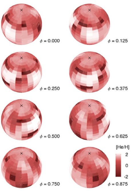
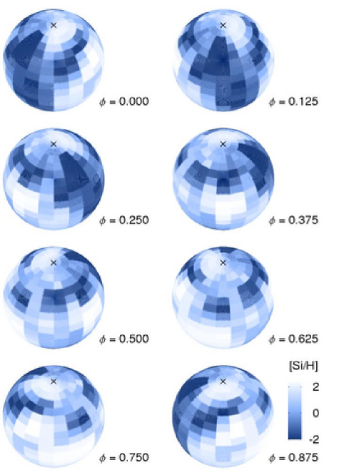
Figure 1: The variation of the helium (left panel) and silicon abundances on the visible disc for different rotational phases (after Khokhlova et al. 2000)

For our study we adopted the surface distribution of He and Si as derived by Khokhlova et al. (2000, see Fig. 1). Here the abundance is defined relatively to the hydrogen, i.e., $[\text{A/H}]=\log(N_{\text{A}}/N_{\text{H}})-\log(N_{\text{A}}/N_{\text{H}})_{\odot}$, where the arguments of the logarithms are number densities of elements A and H on the stellar surface, and on the solar surface respectively. Taking into account that oxygen and iron as derived by Khokhlova et al. (2000) are largely underabundant on the entire surface, we did not consider these elements as sources of the light variability.

2.2 Model atmospheres and photometric colours

We use the standard code TLUSTY (Hubeny 1988; Hubeny & Lanz 1992, 1995; Lanz & Hubeny 2003) for the model atmosphere calculations. We calculate plane-parallel model atmospheres in LTE taking into account bound-bound and bound-free transitions of ions listed in Table 2. We included lighter elements only. Although iron and other iron-peak elements belong to very important sources of opacity in the atmospheres of hot stars, we neglected their influence because iron is, according to Khokhlova et al. (2000), underabundant in the atmosphere of HD~37776 (see also Sect. 5). Because it turns out that the bound-free transitions are important for the variability of HD~37776, we note that the photoionization cross-sections of lighter elements in the TLUSTY ionic models are taken from the Opacity Project (Seaton et al. 1992; Butler et al. 1993, and references therein). Because here we study mainly the effect of helium and silicon, for these elements we used the same models as used in the grid of model atmospheres appropriate to B-type stars calculated by Lanz & Hubeny (2006). Simpler atomic models were used for other elements to speed up the calculation of model atmospheres.

For the spectrum synthesis (from which we calculate the photometric colours) we used SYNSPEC code. We took into account the bound-bound and bound-free transitions for the same ions as for the model atmosphere calculation (see Table 2).

We divided the visible star’s surface into $90\times 360$ elements in latitude and longitude, respectively. We selected such a fine grid just from the numerical reasons to obtain a fairly smooth light curve. The local abundance of helium and silicon (i.e., their number density relatively to the hydrogen) in each surface element was set in accordance with the maps of Khokhlova et al. (2000). The emergent flux from these elements was derived by the interpolation from the model grid. This grid of the model atmospheres contains 80 individual models. The grid is constructed in such a way that for each of the 10 He abundances, 8 different Si abundances were taken according to Table 3. The abundance of other elements for simplicity is assumed to be the solar one (Grevesse & Sauval 1998), i.e., the abundance of elements other than helium and silicon relatively to hydrogen was kept fixed. Note that the effective temperature and surface gravity of all these model atmospheres are set to be the same.

Table 2: Ions and the number of their excitation states considered for the calculation of HD~37776 model atmospheres

Ion	Levels	Ion	Levels	Ion	Levels	Ion	Levels
H i	9	N i	21	Ne i	15	Si ii	40
H ii	1	N ii	26	Ne ii	15	Si iii	30
He i	24	N iii	32	Ne iii	14	Si iv	23
He ii	20	N iv	1	Ne iv	1	Si v	1
He iii	1	O i	12	Mg i	13	S ii	14
C i	26	O ii	13	Mg ii	14	S iii	10
C ii	14	O iii	29	Mg iii	14	S iv	15
C iii	12	O iv	1	Mg iv	1	S v	1
C iv	1

Table 3: Helium and silicon abundances of the model grid

[He/H]	-6	-5	-4	-3	-2	-1	0	1	2		3
[Si/H]				-3	-2	-1	0	1	2	2.5	3

Table 4: Central wavelengths and dispersions of the Gauss filter simulating the transmissivity functions of $uvby$ (Strömgren) photometric system. These values are taken from Cox (2000).

colour	${u}$	${v}$	${b}$	${y}$
${\lambda_{a}}$ [Å]	3500	4100	4700	5500
${\sigma_{a}}$ [Å]	230	120	120	120

We calculate Eddington fluxes $H(\lambda,Y,Z)$ for model atmospheres with helium and silicon abundances $Y$, $Z$ from the grid ($\lambda$ is the wavelength). The flux $H_{c}(Y,Z)$ in a colour $c$ is given by the convolution of $H(\lambda,Y,Z)$ with the transmissivity function of a given filter $c$. The transmissivity function is approximated by a Gauss function peaked at the central wavelength of the colour ${\lambda_{c}}$ with dispersion ${\sigma_{c}}$ (see Table 4). This is performed for each colour $c$ of the $uvby$ system. The radiative flux in a colour ${c}$ from individual surface elements ${H_{c}(\Omega)}$ is obtained by means of interpolation to a proper value of the He and Si abundances of the surface element concerned. Consequently, the flux ${H_{c}(\Omega)}$ is a function of spherical coordinates $\Omega$ on the stellar surface. The total radiative flux observed at the distance $D$ from the star with radius $R_{*}$ is calculated as the integral over all visible surface elements (Mihalas 1978)

$$f_{c}=\left(\frac{R_{*}}{D}\right)^{2}\!\!\int\limits_{\begin{array}[]{c}\text{\scriptsize visible}\\[-5.69054pt] \text{\scriptsize surface}\end{array}}\!\!I_{c}(\theta,\Omega)\cos\theta\,\text{d}\Omega\\ =\left(\frac{R_{*}}{D}\right)^{2}\!\!\int\limits_{\begin{array}[]{c}\text{\scriptsize visible}\\[-5.69054pt] \text{\scriptsize surface}\end{array}}\!\!I_{c}(0,\Omega)u_{c}(\theta)\cos\theta\,\text{d}\Omega\\ =U_{c}^{-1}\left(\frac{R_{*}}{D}\right)^{2}\!\!\int\limits_{\begin{array}[]{c}\text{\scriptsize visible}\\[-5.69054pt] \text{\scriptsize surface}\end{array}}\!\!H_{c}(\Omega)\,u_{c}(\theta)\cos\theta\,\text{d}\Omega,$$ (1)

where $\theta$ is the angle between normal to the surface element and line of sight, $u_{c}(\theta)=I_{c}(\theta,\Omega)/I_{c}(0,\Omega)$ describes the limb darkening (assuming the same limb darkening for each surface element), $I_{c}$ is the intensity in colour $c$ and

$$U_{c}=\frac{1}{4\pi}\int u_{c}(\theta)\cos\theta\,\text{d}\Omega.$$ (2)

Table 5: Calculated limb darkening coefficients (Eq. (3)) in individual colours

colour	${u}$	${v}$	${b}$	${y}$
$a_{c}$	$0.233$	$0.194$	$0.184$	$0.164$
$b_{c}$	$0.163$	$0.216$	$0.204$	$0.177$

For our calculations we use a quadratic limb-darkening law

$$u_{c}(\theta)=1-a_{c}\left(1-\cos\theta\right)-b_{c}\left(1-\cos\theta\right)^{2}.$$ (3)

We adopted the same limb darkening regardless the actual abundance of the surface elements. Namely, the quadratic limb darkening coefficients $a_{c}$, $b_{c}$ in each colour $c$ were derived from the solar abundance model. Different methods are available for the derivation of limb darkening coefficients (e.g. Grygar et al. 1972). We selected a method similar to Wade & Rucinski (1985), which conserves the total flux. This leads to a condition

$$b(\lambda)=6-2a(\lambda)-\frac{24H(\lambda)}{I(\lambda,\theta=0)},$$ (4)

where $H(\lambda)$ is the emergent Eddington flux and $I(\lambda,\theta=0)$ is the emergent intensity at the $\theta=0$ ray. The value of the coefficient $a$ is derived by the least-square fitting of Eq. (3) with the condition Eq. (4) to values of $u_{i}(\lambda)$ calculated using SYNSPEC for different angles $\mu_{i}$. For the least-square fitting we used weights equal to angles $\mu_{i}$. This leads to a formula

$$a=\frac{\sum\mu_{i}(1-\mu_{i})(1-2\mu_{i})\left[\left(6-\frac{24H}{I(0)}\right)(1-\mu_{i})^{2}-1+u_{i}\right]}{\sum\mu_{i}(1-\mu_{i})^{2}(1-2\mu_{i})^{2}},$$ (5)

where we, for abbreviation, dropped the wavelength dependence of all quantities. The limb darkening coefficients in each colour $a_{c}$, $b_{c}$ were derived from Eqs. (4), (5) using the gaussian smoothing over the colour $c$ with parameters taken from Table 4. Bound-bound transitions in the calculation of $u_{c}$ were also taken in to account. The calculated linear limb darkening coefficients are given in Table 5.

Finally, the observed magnitude difference is

$$\Delta m_{c}=-2.5\,\log\,\left(\frac{{f_{c}}}{f_{c}^{\mathrm{ref}}}\right),$$ (6)

where $f_{c}$ is calculated from Eq. (1) and ${f_{c}^{\mathrm{ref}}}$ is the reference flux obtained from the condition that the mean magnitude over the phase is zero. As the spectral energy distribution within the width of a Strömgren filter is affected by the interstellar reddening only marginally, provided that e. g. after Shore & Brown (1990) $E(B-V)=0.081$, we can neglect the influence of the interstellar reddening. Note that the interstellar reddening influences mainly the difference between two colours (the colour index), not the value of the change in a given colour.

The calculation of magnitudes after Eq. (6) is performed over $36$ rotational phases.

3 Influence of chemical peculiarity on emergent fluxes

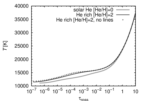
Figure 2: The dependence of the temperature on the Rosseland optical depth $\tau_{\text{ross}}$ in the atmospheres with various chemical compositions. Crosses denote the case of atmosphere with enhanced abundance of either silicon or helium, however neglecting the opacity due to the line transitions of these elements.

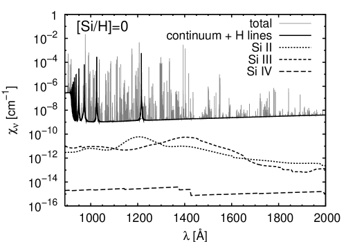
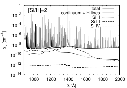
Figure 3: Different sources of the opacity at the point where $\tau_{\text{ross}}\approx 1$ for the solar chemical composition (left panel) and for [Si/H]=2. In the silicon overabundant atmosphere the bound-free transitions due to higher excited levels of Si ii and Si iii become important sources of the opacity in the far UV region of the Balmer continuum.

As a result of higher opacity in the models with enhanced abundance of either helium or silicon, the temperature in the outer parts of the atmosphere increases due to the backwarming. This can be seen in the plot of the dependence of the temperature on the Rosseland optical depth $\tau_{\text{ross}}$ for atmospheres with different chemical compositions in Fig. 2. To identify the main source of the opacity responsible for the backwarming we also calculated atmosphere models neglecting the contribution of He-Si lines. Apparently, the line transitions influence the atmosphere temperature only for $\tau_{\text{ross}}\lesssim 10^{-3}$, where the stellar atmosphere is basically transparent in continuum. Consequently, the main influence of the enhanced abundance of helium and silicon on the atmosphere temperature stratification (in the region where the photometric flux forms, i.e., for $0.1\lesssim\tau_{\text{ross}}\lesssim 1$) is due to bound-free transitions. Indeed, as demonstrated in Fig. 3, in the case of silicon overabundance, the bound-free transitions from the higher excited levels of Si ii and Si iii significantly contribute to the continuum opacity in the wavelength region where most of the flux is radiated from the atmosphere of HD~37776, i.e., in the far UV region of the Balmer continuum.

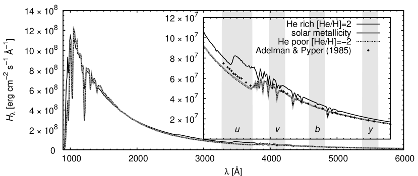
Figure 4: The emergent flux from the atmospheres with different helium abundances. The flux was smoothed by a Gaussian filter with a dispersion of $10\,\AA$ to show the changes in continuum, which are important for photometric variability. The passbands of the $uvby$ photometric system are also shown on the graph (gray area). The photometric region was also enlarged and overplotted. For a reference we show also the observed mean flux derived by Adelman & Pyper (1985), which we normalize using the predicted solar-abundance flux at 5000 Å.

Figure 5: The same as Fig. 4, for silicon.

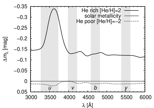
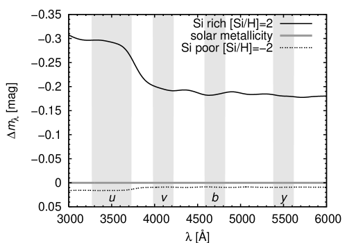
Figure 6: The magnitude difference between the flux at the given abundance of helium (left panel) and silicon (right panel) $H(\lambda,Y,Z)$ and the flux for the solar abundance $H(\lambda,Y_{\odot},Z_{\odot})$ calculated as $\Delta m_{\lambda}=-2.5\log(H(\lambda,Y,Z)/H(\lambda,Y_{\odot},Z_{\odot}))$. The passbands of the $uvby$ photometric system are also shown on the graph (gray area). The flux was smoothed by a Gaussian filter with dispersion 120 Å to show the changes in the wavelength range corresponding to the pass-bands of the $u$, $v$, $b$ and $y$ filters.

The radiative flux emerging from the model atmospheres depends on the silicon and helium abundances, as can be seen in Figs. 4, 5. For solar chemical composition, the Balmer jump is visible in the plot. With increasing silicon abundance, the opacity in the ultraviolet (UV) region below roughly $1600\,$Å increases mainly due to bound-free silicon transitions (and partly also due to the bound-bound transitions, see Fig. 3). The flux from this UV region is redistributed towards longer wavelengths, partly into the optical region. Consequently, the silicon overabundant regions are brighter than the silicon poor ones in the $uvby$ bands. A very similar situation occurs also in the case of helium overabundance. However, since for [He/H]=$2$ the helium dominates in the stellar atmosphere, jumps due to ionization of neutral helium occur. Helium overabundant regions are also brighter in the $uvby$ bands than those with lower helium abundance. Decreased helium and silicon abundances below the solar values outside the bright spots do not significantly influence the flux in the $uvby$ colours. As a result, we expect that only bright spots occur on the stellar surface, not the dark ones that may seemingly originate only due to a contrast effect.

There is a relatively good agreement between the shapes of the calculated and predicted spectral energy distribution (for solar abundance) in the visible region (taken from Adelman & Pyper 1985, note that from the observations only fluxes expressed relatively to the flux at $5000\,$Å are available). The observed fluxes are slightly higher than the predicted ones in the Lyman continuum just below the Balmer jump. This difference might reflect the influence of the chemical peculiarity.

To identify the main sources of the light variability, we compared the fluxes calculated using models with neglected line transitions with that ones calculated with inclusion of the line transitions. This comparison showed that the line transitions contribute to the light amplitude only by up to percents.

The change of the fluxes manifests itself through the change of the apparent magnitude, Fig. 6. The change is nearly the same in the $b$ and $y$ colours, which is caused by the fact that these colours lie on the Wien part of the energy distribution function and no important ionization edges are located there. The different change in the $u$ colour is connected with the behaviour of the Balmer jump and the occurrence of the jump due to helium ionization. The change in the $v$ colour may be also slightly influenced by the presence of the Balmer jump.

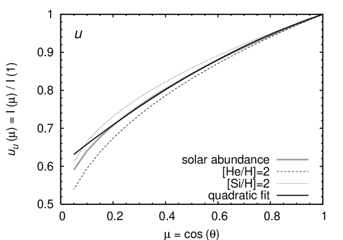
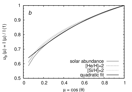
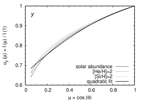
Figure 7: The continuum limb darkening at the wavelength corresponding to the center of the individual filter (Tab. 4) in the model atmospheres with different chemical composition. The solid black line denotes the quadratic limb darkening (see Eq. (3), taking into account also lines) adopted in this paper.

The change of the chemical composition of the atmosphere also influences the limb darkening as shown in Fig. 7. However, near the disk center for $\cos\theta>0.6$ the variations of the limb darkening with abundance are not so significant. Consequently, we did not include these changes into our modelling, because the approximation of the limb darkening does not have a significant influence on the calculated light curves. For example, out test showed that there is only a relatively small difference, up to $\approx 0.001$ mag, between the light curves calculated using quadratic and linear limb darkening.

4 Simulation of the light curve

4.1 Helium

Since helium is the dominant element in the majority of regions on the HD~37776 surface (Khokhlova et al. 2000), we started studying the light variations caused by this element only. The corresponding light curves calculated taking into account the uneven distribution of helium on the HD~37776 surface (and the solar chemical composition of other elements) are given on Fig. 8. Because the most helium-rich regions appear on the visible disk during the light minimum of the observed light variations, and because the helium overabundance induces the brightening of the stellar surface (Fig. 4), the predicted light variations caused by helium are practically in antiphase with the observed ones. Consequently, although helium significantly contributes to the light variability of HD~37776, there has to also be another mechanism that dominates the optical variability of this star.

To check the response of the light curve to the various values of the abundance of helium we reduced it by 1 dex relative to the value derived by Khokhlova et al. (2000). This, however, did not induce a remarkable change, as seen in Fig. 8. This is due to the fact that even with [He/H]=1 the atmosphere starts to be dominated by helium already.

4.2 Silicon

Figure 8: The simulated light variations of HD~37776 in different colours derived taking into account only the uneven distribution of helium on its surface (solid line) compared with individual $uvby$ observations (Pedersen & Thomsen 1977; Adelman & Pyper 1985; Adelman 1997). The dotted line denotes the simulated light curve derived taking into account the helium abundance reduced by $1\,$dex. All observed magnitudes are shifted in such a way that their mean value is zero. A vertical offset of 0.05 mag was applied between each consecutive filter.

Figure 9: The same as Fig. 8, taking into account only the uneven distribution of silicon. The dotted line denotes the light curve calculated for the surface distribution of silicon derived from the observations by Khokhlova et al. (2000) decreased by $0.5\,$dex. A vertical offset of 0.05 mag was applied between each consecutive filter.

The fact that silicon is overabundant on the observed disc around the phase $\phi=0.75$, when the star has its light maximum (Adelman 1997, see also Fig. 9 and Fig. 1), along with our finding that silicon rich regions are bright, lead us to deduce that silicon may be the main cause of the HD~37776 variability. To test this, we calculated the light curve of HD~37776 taking into account only the uneven distribution of silicon (Khokhlova et al. 2000). The resulting light curve is displayed in Fig. 9. Apparently, taking into account only the uneven surface distribution of silicon, the amplitude of the light curve is too large when compared with the observed one (especially in the $u$ colour). However, there is a good agreement between the light curve shapes. Note also that the amplitude is relatively sensitive to the value of [Si/H].

4.3 Helium and silicon

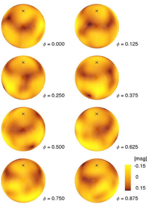
Figure 10: The location of the calculated photometric spots in the $u$ colour. We plot the smoothed flux emergent from the individual surface elements calculated using the observed surface distribution of helium and silicon derived by Khokhlova et al. (2000) in magnitudes. Here we do not include the limb darkening.

Figure 11: The same as Fig. 8, taking into account the uneven surface distribution of both the helium and silicon (solid line). A vertical offset of 0.05 mag was applied between each consecutive filter.

The promising correspondence between the observed and predicted light curves derived above encourages us to include both silicon and helium in the calculation of the light curve. To visualize the origin of the light variations, we plot the photometric spots on the surface of HD~37776 in different rotational phases in Fig. 10 in the $u$ colour. As it follows from this plot the shape of the light curve significantly depends on the inclination $i$.

Inspecting Figs. 6, 8 we can conclude that the variations due to helium and silicon are basically in the antiphase. Consequently, helium may suppress the too large amplitude derived assuming silicon surface variations only (especially in the $u$ colour see Fig. 9). Indeed, the computed light curve shown in Fig. 11, where both silicon and helium abundance variations are taken into account, confirms these considerations. There is a very good agreement between the predicted and observed light curves in the shape and amplitude. There is just a relatively small disagreement in the $u$ colour. Some part of the remaining discrepancy between the predicted and observed curves may be due to uncertainties of spots location as derived from observations, as the observed maps are tabulated at relatively coarse interval of $18^{\circ}$ in longitude.

Consequently, we conclude that the observed light variability of HD~37776 can be successfully simulated assuming the uneven surface distribution of individual elements, mostly silicon and helium.

5 Discussion

The role of other elements

An uneven surface distribution of elements other than silicon and helium may influence the light curve. Whereas the influence of oxygen and iron, which are underabundant on the HD~37776 surface (Khokhlova et al. 2000), is likely to be negligible, other elements (especially carbon for which the spectral line variability is observed, see Shore & Brown 1990) may modify the predicted light curve. On the other hand, if the iron abundance is much higher than what we assumed, then the iron opacity could be important for the spectral energy distribution and variability (provided the uneven surface distribution of iron). We note that Khokhlova et al. (2000) derived from Doppler-Zeeman mapping that iron is relatively most abundant in spots where its deficit reaches up to 2 dex, while in the rest of the atmosphere the deficit is 4 – 5 dex relative to the solar value. These values are surprisingly low and deserve further investigation using model atmospheres with magnetic fields included.

NLTE effects

The NLTE effects have a significant influence on the spectra of hot stars. These effects influence mainly the state of the outermost parts of the stellar atmospheres, where the lines are formed, and which is optically thin in the visible continuum. Since Khokhlova et al. (2000) used LTE models for mapping of the HD~37776 surface (and, consequently, the real abundances may be different), we use also the LTE models here. The neglect of the NLTE effects for both the abundance determination and synthetic spectrum calculation may be one of the reasons of the remaining small discrepancy in the $u$ colour.

Influence of the magnetic field

Staude (1972) and Trasco (1972) showed that a strong surface magnetic field may influence the emergent spectral energy distribution which may in photometry amount to hundredths of magnitude. Khan & Shulyak (2006) and Kochukhov et al. (2005) studied the influence of the polarized radiative transfer and magnetic line blanketing on the energy distribution, atmospheric structure and photometric colours and showed the magnetic field has a clear relation to the visual flux depression. Stȩpień (1978) deduced that the effect of the magnetic field on the stellar atmosphere leads to variation of $T_{\rm eff}$ and $\log g$ over the stellar surface resulting in light variations. Consequently, the surface variations of the magnetic field may also contribute to the light variability.

Vertical distribution of elements

The vertically dependent abundance variations in chemically peculiar stars are suggested by many authors (e.g., Ryabchikova 2004). This effect may also influence our results, because the effective depth at which the lines form (i.e., at which the abundance map is in fact derived) differs from that at which continuum forms (i.e., at which the light variations are formed). Moreover, the chemical stratification itself may influence the emergent continuum flux. However, to our knowledge, no evidence of the vertical chemical stratification is available for HD~37776 atmosphere at the present time.

Uncertainties of stellar parameters

Uncertainties of the determination of the stellar parameters may influence the comparison between observed and predicted quantities. However, since we study mainly differential flux variations in individual colours, the influence of the determination of, e.g., the surface gravity acceleration or the stellar effective temperature are likely to be less important. Indeed, the comparison of the the magnitude differences calculated for [Si/H]=2 after Eq. 6 for stellar model calculated with the effective temperature by $1000\,$K lower or the surface gravity by $0.5\,$dex higher shows that the magnitude differences vary by about $0.02\,$mag (compare with the change of $0.1-0.35\,$mag showed in Fig. 6). The magnitude differences are even less sensitive to the changes of the turbulent velocity, because the increase of the turbulent velocity by $2\,\text{km}\,\text{s}^{-1}$ causes the variation of the magnitude difference by only about $0.001\,$mag.

Alternative surface chemical composition maps

Because with the helium-only overabundance model we came up with a big discrepancy between the computed and observed light curves (Fig. 8), we used another available model derived for the surface chemical composition of helium only, by Vetö et al. (1991). However, neither with this different surface pattern we were able to reproduce the observed light curve (cf. Fig. 8). A further map of the surface chemical composition which can be used for the reliable simulation of the light curve is that of Bohlender & Landstreet (1988). To test the influence of independent surface chemical composition map on our result, we used the original map derived by Khokhlova et al. (2000), however the maximum and minimum abundances of helium and silicon were taken from Bohlender & Landstreet (1988). Generally, as a result of lower silicon abundance in the spot (compared with that by Khokhlova et al. 2000), the amplitude due to silicon is lower when using Bohlender & Landstreet (1988) silicon abundance. However, this is compensated by lower maximum helium abundance. Consequently, our tests showed that also with this different surface map we are able to obtain a fair agreement with observations.

Light variations in UV

If the proposed mechanism of the light variability is correct, the studied star should be variable also in the UV region and the observed light curve in the far UV region should be in antiphase with the optical and near-UV light curve. Indeed, a similar behaviour was found for other CP stars CU Vir and 56 Ari by Sokolov (2000, 2006).

Comparison with observed flux distribution

The next step in the comparison of the observed and predicted characteristics would be to compare the mean observed average flux derived by Adelman & Pyper (1985) and the theoretical one. Whereas there is a good agreement between these fluxes in the visible region, there is a slight disagreement (less than $10\%$) between them in the region between helium and hydrogen ionization edges in the $u$ colour. The enhancement of the mean predicted flux in this region is caused by the enhanced helium abundance. Consequently, this might indicate that the maximum helium abundance on HD~37776 surface is lower than that reported by Khokhlova et al. (2000). We also note that, for example, the effective temperature of HD~37776 was obtained using atmosphere models with solar chemical composition, which are unrealistic in the case of helium dominated atmosphere. However, the detailed study of this problem is beyond the scope of the present paper, which is concerned with the flux variations in individual passbands and not in the differences between magnitudes of individual passbands.

Light absorption (extinction) in the circumstellar environment

Townsend et al. (2005) were able to simulate successfully the light curve of another helium-rich chemically peculiar star $σ$~Ori~E (see also Nakajima 1985; Smith & Groote 2001) using the model of rigidly rotating magnetosphere (Townsend & Owocki 2005). However, we argue that our model of a rotating spotted star is more convenient for HD~37776. First, our method allows the simulation of the light curve just from the surface chemical distribution and we do not use any free parameter to fit the amplitude. Second, the light curve of HD~37776 is quite different from that of $\sigma$ Ori E, which shows deep and relatively narrow minima with maximum amplitude in the $u$ (Pedersen & Thomsen 1977). Finally, $\sigma$ Ori E is known for its emission in H$\alpha$ line (Walborn 1974), which is absent in the case of HD~37776. The uneven distribution of chemical elements on the surface of $\sigma$ Ori E (Reiners et al. 2000) may, however, also influence the light curve of $\sigma$ Ori E and may explain some secondary effects which are not explained by the cloud absorption model.

Light variations of other chemically peculiar stars

Since silicon is overabundant in the majority of chemically peculiar stars that show light variations (Si, He-weak, and He-strong stars, very frequently cool CP stars, e.g., Adelman 1973) it may play a crucial role also in their variability. However, this has to be tested also for other CP stars, as, e. g. Carpenter (1985) showed that the anomalous Zeeman effect is capable to induce such an enhancement of the Si ii 4131Å without the need of the large overabundance of the element.

6 Conclusions

In this work we were able to explain consistently the light curve of He-strong chemically peculiar star HD~37776. The observed light variations are explained in terms of the uneven surface distribution of helium and silicon. The helium and silicon spots modify the emergent flux predominantly due to the bound-free transitions. The predicted light curves reproduce the observed ones very well in their overall shape and amplitude. Although the agreement between the observed and predicted light curves may seem satisfactory, we stress that there are also other effects (e.g., NLTE effects, influence of other chemical elements) that may be important for the light curve.

We have shown that bound-free transitions of mainly heavier elements (in our case silicon) accompanied with uneven surface distribution of these elements are crucial for the light variability of magnetic chemically peculiar stars. To our knowledge, this mechanism has never been invoked in the literature to predict the light variability.

Our results are important not only from the point of view of explanation of light curves of chemically peculiar stars, but the comparison of predicted and observed light curves represents an important check of model atmospheres and their predictions.