Lateral Effects in Fermion Antibunching

Abstract

Lateral effects are analyzed in the antibunching of a beam of free non-interacting fermions. The emission of particles from a source is dynamically described in a 3D full quantum field-theoretical framework. The size of the source and the detectors, as well as the temperature of the source are taken into account and the behavior of the visibility is scrutinized as a function of these parameters.

I Introduction

The wave function of two fermions is antisymmetric under exchange of the two particles, as a consequence of the Pauli exclusion principle. For this reason, the probability amplitude for their being spatially close together is small and their correlated detections are reduced when compared to a random sequence of classical particles. This very distinctive quantum feature is named antibunching and has no classical analog. Notice that in general the two particles can be emitted from totally incoherent sources.

The analogous phenomenon for bosons is a cornerstone in the study of quantum correlations and was first observed in astronomy, where it is known as the Hanbury Brown-Twiss effect HBT . Photon second-order coherence effects sudarshan ; glauber ; bargmann , yielding bunching, are discussed in physics textbooks Loudon ; MandelWolf , and led to novel interesting applications in quantum imaging como ; UMBC and lithography litho .

The most relevant difference between the Bose-Einstein and Fermi-Dirac statistics are the phase space densities (occupation numbers), that change by several orders of magnitude. In a laser beam, one obtains values of order $10^{14}$, while typical densities for thermal light, synchrotron radiation and electrons are of order $10^{-3}$; finally, for the most advanced neutron sources, one gets $10^{-15}$. These figures make it very difficult to observe fermion antibunching. In addition, for charged particles (electrons and pions), additional Coulomb repulsion effects should be considered, that tend to reduce the visibility and mask the observation of the phenomenon.

Quantum correlations have been detected in a series of interesting experiments: in condensed-matter physics, where the electronic states are confined within the Fermi surface electron1 ; electron2 ; electron3 , for superconductor emitters Oshima , in the coincidence spectrum of neutrons from compound-nuclear reactions at small relative momentum tre ; qua , as well as in pion pairs emitted from a quark-gluon plasma CERN . Recently, antibunching was observed on a beam of thermal neutrons emitted from a nuclear reactor IOSFP . This can be considered as a direct experimental evidence of free fermion antibunching, in which an ensemble of free Fermi particles displays quantum coherence effects. Other remarkable antibunching experiments have been recently reported for neutral atoms, both in a degenerate atomic Fermi gas atom and in Fermi/Bose gases He .

Huge numerical differences in phase space densities, like the afore-mentioned ones, call for close scrutiny of the theoretical premises as well as dedicated experimental efforts. Notice that these quantum statistical effects appear to play a prominent role in phenomena that are characterized by figures that differ by almost 30 (!) orders of magnitude. The present study is motivated by this observation. We intend to analyze the antibunching phenomenon in the correlated detections of two neutral fermions, such as neutrons, emitted by a generic thermal source at a given temperature. Notice that bunching effects from (pseudo-)thermal sources still raise controversial interpretations thermalcontrov and are therefore worth investigating from first principles.

Our main objective will be to analyze the spatial coherence and in particular the coherence area and volume. Lateral effects are becoming a critical issue, in view of a new generation of experiments. They were carefully analyzed in a series of experimental articles on X-ray bunching SPring8 . For the sake of concreteness, we will focus on fermions, but our analysis can be very easily extended to bosons (by replacing the energy distributions of the source and changing relevant signs in the formulas).

We will treat both the source (a thermal oven) and the particle beam as fully (second) quantized systems and will study the emission process at thermal equilibrium, when the beam has reached its stationary configuration. This approach will have the advantage of treating both the oven and the fermion beam on an equal footing and of introducing the properties of the source in a natural way.

II Setup and Outline

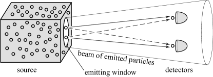
Before starting a detailed analysis, let us outline the main features of the setup we have in mind and stress the main points of our argument. Our setup is the simple one schematically shown in Fig. 1. Particles are emitted from a source through a small window, go through a monochromator (not shown), and are detected by two detectors. We count the number of coincident detections. At the initial time $t=0$, the source is in the thermal equilibrium state at a finite temperature and outside there is the vacuum. Starting from this initial condition, we shall solve the dynamics of the emission, so that a stationary beam of particles will be prepared at $t\to\infty$, after a transient period. The beam profile will not be added “by hand,” but will be obtained by solving the equations of motion, so that the coherence properties of the emitted particles will reflect the dynamics of the emission.

The lateral features of the system affect the antibunching, even when both detectors are placed on the longitudinal axis and we shall look at the correlation in the longitudinal direction. To this end, the lateral size of the detector mouth must be duly taken into account. We shall therefore implement the lateral resolution of the detector, as well as the longitudinal one, in the two-particle distribution function. The variables and parameters that characterize the setup are summarized in Table 1.

Figure 1: Coincidence between two detectors in the beam of emitted particles: the interference of the two alternatives yields antibunching.

We shall start by writing down the Hamiltonian of this many-body system in Sec. III. This is the crucial part of the present analysis, since it fully relies on dynamical consideration. In order to facilitate the introduction of the characteristics of the source, like temperature, size of the window, and so on, in a natural way, we shall adopt a two-field approach: one field describes the particles in the source and the other one the emitted particles outside. The emission Hamiltonian $\lambda H_{\text{emission}}$ (which converts a particle in the source into a particle outside and vice versa) is at the heart of our analysis and must fully take into account all important features of the experimental setup, as well as the main characteristics of the physics of the emission process. The Hamiltonian below will enable us to discuss the lateral coherence features of the emitted beam, yet it will be simple enough to be (almost) solvable. As we will see, the diffraction of the particles emitted through the window governs the lateral coherence and is controlled by the lateral size of the emitting window. Once the Hamiltonian is written down, one has “only” to solve the equations of motion (and has no “freedom” anymore).

The article is organized as follows. The dynamics of the emission is perturbatively solved in Sec. IV, under the assumption of weak emissivity, namely weak coupling $\lambda\ll 1$, and the stationary limit $t\to\infty$ realizes a nonequilibrium steady state. The beam profile thus prepared is studied at a large distance from the source in Sec. V. We then compute the two-particle distribution function, or in other words, the second-order correlation function, defined in Sec. VI. The interplay between the singlet and triplet contributions determines to which extent the coincidence counts are reduced (antibunching) when the two detectors are close to each other. Indeed, the singlet contribution yields bunching and the triplet one antibunching, with the latter three times larger than the former. The detector sizes (resolutions) $a$ and $d$ are implemented into the correlation functions, the saddle-point approximation is carefully worked out for the case in which the detectors are placed on the longitudinal $z$ axis, and we obtain a formula for the normalized two-particle distribution function. The noncollinear case, with the two detectors placed off the longitudinal axis, is also discussed.

The antibunching is then discussed and the coherence properties are clarified in Sec. VII, on the basis of our formula for the collinear case, and the effect of the temperature of the source is scrutinized. The temperature effect is shown to be very weak. The dependence of the antibunching correlation function on the distance between the two detectors is found to be controlled by the lateral monochromator window and the longitudinal detector resolution, while the magnitude of the antibunching effect is determined by the lateral size of the source. Finally, a variety of experiments are analyzed in Sec. VIII, in the light of the lateral coherence, and the main results are summarized in Sec. IX.

Table 1: Summary of the variables and parameters used in the calculation.

$z$	longitudinal direction
$x,y$	transverse directions
$w$	lateral size of the circular emitting window of the source
$w_{z}$	depth of the emitting region
$\bm{k}_{0}$	average momentum at monochromator
$\delta k_{i}$ ($i=\perp,z$)	monochromator window
$a$	lateral size of the circular mouth of the detector
$d$	detector resolution in the longitudinal direction
$0$ (origin)	center of the emitting region
$\bar{\bm{r}}_{i}$ ($i=1,2$)	centers of detector apertures
$\beta$	inverse temperature of the source
$\mu$	Fermi level (in the source)
$g(\bm{r})$	emitting window function
$f(\bm{k})$	monochromator momentum-window function
$R_{\bar{\bm{r}}}(\bm{r})$	detector resolution function

III Hamiltonian and State of the Source

Let us start with the Hamiltonian: we take

$$H=H_{0}+\lambda H_{\text{emission}},\quad H_{0}=H_{\text{beam}}+H_{\text{source}},$$ (1a)

where

$$H_{\text{beam}}=\sum_{\sigma=\uparrow,\downarrow}\int\text{d}^{3}\bm{k}\,\varepsilon_{k}c_{\bm{k}\sigma}^{\dagger}c_{\bm{k}\sigma},\quad H_{\text{source}}=\sum_{\sigma=\uparrow,\downarrow}\int\text{d}^{3}\bm{k}\,\omega_{k}a_{\bm{k}\sigma}^{\dagger}a_{\bm{k}\sigma},$$ (1b)

$$H_{\text{emission}}=\sum_{\sigma=\uparrow,\downarrow}\int\text{d}^{3}\bm{k}\int\text{d}^{3}\bm{k}^{\prime}\,\Bigl{(}T_{\bm{k}\bm{k}^{\prime}}c_{\bm{k}\sigma}^{\dagger}a_{\bm{k}^{\prime}\sigma}+T_{\bm{k}\bm{k}^{\prime}}^{*}a_{\bm{k}^{\prime}\sigma}^{\dagger}c_{\bm{k}\sigma}\Bigr{)}.$$ (1c)

Not only the emitted particles but also the source is treated as a second quantized dynamical system. The Hamiltonian of the particles in the source is $H_{\text{source}}$ and that of the emitted particles is $H_{\text{beam}}$. The emission is dynamically described by an emission Hamiltonian $\lambda H_{\text{emission}}$: a particle of momentum $\bm{k}^{\prime}$ and spin $\sigma$ is annihilated by $a_{\bm{k}^{\prime}\sigma}$ in the source and is created by $c_{\bm{k}\sigma}^{\dagger}$ outside with an amplitude $\lambda T_{\bm{k}\bm{k}^{\prime}}$, the meaning of which will be described below. The creation and annihilation operators obey the canonical anticommutation relations for fermions

$$\{c_{\bm{k}\sigma},c_{\bm{k}^{\prime}\sigma^{\prime}}^{\dagger}\}=\{a_{\bm{k}\sigma},a_{\bm{k}^{\prime}\sigma^{\prime}}^{\dagger}\}=\delta_{\sigma\sigma^{\prime}}\delta^{3}(\bm{k}-\bm{k}^{\prime}),\qquad\{c_{\bm{k}\sigma},a_{\bm{k}^{\prime}\sigma^{\prime}}^{\dagger}\}=0.$$ (2)

It is assumed that no spin flip occurs during the emission process and that the emission is irrespective of the spin state of the particle ($T_{\bm{k}\bm{k^{\prime}}}$ does not depend on $\sigma$): generalizations to more general cases are straightforward. The field operator in the configuration space for the emitted particles is denoted by

$$\psi_{\sigma}(\bm{r},t)=\int\frac{\text{d}^{3}\bm{k}}{\sqrt{(2\pi)^{3}}}\,c_{\bm{k}\sigma}\text{e}^{\text{i}(\bm{k}\cdot\bm{r}-\varepsilon_{k}t)}.$$ (3)

In the following discussion, the dispersion relations are assumed to be $\varepsilon_{k}=\omega_{k}=\bm{k}^{2}/2m$.

In Eq. (1), $\lambda$ is a small parameter, that will enable us to work in the weak-coupling limit. Although this approach is familiar in variety of theoretical approaches aimed at explaining diverse experimental situations, a few words of explanation are necessary in this case. We have in mind a situation in which an oven emits a beam of particles through a small aperture (which we refer to as “source”). Usually, those particles that leave the source are monochromatized and can travel in waveguides, undergoing all kinds of losses. The parameter $\lambda$ globally accounts for all these diverse processes and $\lambda H_{\text{emission}}$ simply enables us to take a particle with approximately the right characteristics in the oven and put it in the final section of the beam. The smallness of the opening and the total “efficiency” of the emission process (from the oven to the region of space where the experiment is practically done, passing through monochromators, optical elements and/or waveguides and undergoing losses) calls for an approach in which $\lambda$ is a small parameter. We anticipate that in all final formulas, where normalized distribution functions will be studied, $\lambda$ will always simplify, making the final results independent of the details of the apparatus (such as the monochromatization procedure, reflection and transmission processes, losses in optical elements and waveguides and so on). Of course, one must be able to retain all essential elements in the analysis and final formulas. The quantity $T_{\bm{k}\bm{k}^{\prime}}$ in Eq. (1c) takes into account the action of the monochromator and the size of the source, and will be defined in Eq. (5).

The Hamiltonian discussed in this section is to be considered as a phenomenological transfer Hamiltonian, conveniently tailored in order to discuss lateral size effects. It is similar to a “tunneling” Hamiltonian (for a two-field formulation of a tunneling process, see tunneling ) and can describe the particle emission from a small opening.

III.1 Emission

We consider the following emission process. Only the particles around the window of the source are emitted outside. That is, a particle in the momentum state $|{\bm{k}}\rangle$ (with $k_{z}>0$) is annihilated by $a_{\bm{k}\sigma}$ around the window of the source and is converted into a particle outside by $c_{\bm{k}^{\prime}\sigma}^{\dagger}$. The emitting region is specified by a function $g(\bm{r})$ centered around the window of the source that characterizes the lateral size of the window. One may further put a monochromator $f(\bm{k})$ after the emission. The emission Hamiltonian is then given by

$$H_{\text{emission}}=\sum_{\sigma=\uparrow,\downarrow}\int\text{d}^{3}\bm{k}^{\prime}\int\text{d}^{3}\bm{k}\,c_{\bm{k}^{\prime}\sigma}^{\dagger}\langle{\bm{k}^{\prime}}|f(\bm{k})g(\bm{r})\theta(k_{z})|{\bm{k}}\rangle a_{\bm{k}\sigma}+\text{h.c.}$$ (4)

with the emission matrix

$$T_{\bm{k}^{\prime}\bm{k}}=\langle{\bm{k}^{\prime}}|f(\bm{k})g(\bm{r})\theta(k_{z})|{\bm{k}}\rangle=f(\bm{k}^{\prime})\theta(k_{z})\int\frac{\text{d}^{3}\bm{r}}{(2\pi)^{3}}\,g(\bm{r})\text{e}^{-\text{i}(\bm{k}^{\prime}-\bm{k})\cdot\bm{r}}=f(\bm{k}^{\prime})\tilde{g}(\bm{k}^{\prime}-\bm{k})\theta(k_{z}).$$ (5)

The theta function, $\theta(k_{z})=1$ for $k_{z}>0$ and $\theta(k_{z})=0$ for $k_{z}<0$, accounts for the positivity of the longitudinal momentum $k_{z}$. In the following calculation, we assume Gaussian shapes for the emitting region and the monochromator,

$$g(\bm{r})=\frac{1}{\sqrt{(2\pi)^{3}\det\mathcal{W}^{2}}}\text{e}^{-\bm{r}\cdot\mathcal{W}^{-2}\bm{r}/2},\quad\mathcal{W}^{2}=\begin{pmatrix}w^{2}&0&0\\ 0&w^{2}&0\\ 0&0&w_{z}^{2}\end{pmatrix},$$ (6)

$$f(\bm{k})=\frac{1}{\sqrt[4]{(2\pi)^{3}\det(\delta\mathcal{K})^{2}}}\text{e}^{-(\bm{k}-\bm{k}_{0})\cdot(\delta\mathcal{K})^{-2}(\bm{k}-\bm{k}_{0})/4},\quad(\delta\mathcal{K})^{2}=\begin{pmatrix}(\delta k_{\perp})^{2}&0&0\\ 0&(\delta k_{\perp})^{2}&0\\ 0&0&(\delta k_{z})^{2}\end{pmatrix},$$ (7)

where $w$ represents the lateral size of the window of the source, $w_{z}$ is the depth of the emitting region, and $\delta k_{i}$ ($i=\perp,z$) characterize the monochromator. In the following, we shall take $\bm{k}_{0}=(0,0,k_{0})$.

It is interesting to notice that the non-factorized form (5) of the interaction Hamiltonian will produce the required diffraction effect. (A factorized emission Hamiltonian would correspond to a point source, irrespectively of the state before the emission, and would not yield the desired lateral effect. The choice of the Hamiltonian and the validity of our working assumptions will be continuously checked throughout the whole calculation.) A particle with momentum $\bm{k}$ in the source is converted into a particle with momentum $\bm{k}^{\prime}$ outside. The momentum transfer is governed by the Fourier transform $\tilde{g}(\bm{k}^{\prime}-\bm{k})$ of the “interface” function $g(\bm{r})$ and is ruled by the size of the window. A smaller window yields larger momentum transfer and results in a larger divergence of the emitted beam. This point will be crucial in the following discussion on the lateral coherence of the beam. The beam profile is therefore a direct consequence of the dynamics and is not artificially imposed at the outset. We also notice that the longitudinal component of momentum is not necessarily preserved during the emission process, as conservation of the longitudinal momentum prevents beam divergence. This motivates the choice of the form factor.

III.2 State of the Source

Having written the Hamiltonian of the emission process, it is straightforward to introduce also the properties of the source. The initial thermal state of the source at a finite temperature $\beta^{-1}$ is characterized by

$$\langle a_{\bm{k}\sigma}^{\dagger}a_{\bm{k}^{\prime}\sigma^{\prime}}\rangle=N(\omega_{k})\delta_{\sigma\sigma^{\prime}}\delta^{3}(\bm{k}-\bm{k}^{\prime}),\qquad N(\omega)=\frac{1}{\text{e}^{\beta(\omega-\mu)}+1}.$$ (8)

In the present article, we shall focus for concreteness on the Fermi distribution. However, we can think of a more general distribution $N(\omega_{k})$. In fact, many of the formulas below remain valid as long as the initial state is stationary with respect to $H_{0}$, admits the Wick decomposition, and $N(\omega_{k})$ is a slowly varying function around $k_{0}$.

IV Dynamics of Emission

The Heisenberg equations of motion read

$$\begin{cases}\vskip 6.0pt plus 2.0pt minus 2.0pt\displaystyle\text{i}\frac{\text{d}}{\text{d}t}c_{\bm{k}\sigma}(t)=\varepsilon_{k}c_{\bm{k}\sigma}(t)+\lambda\int\text{d}^{3}\bm{k}^{\prime}\,T_{\bm{k}\bm{k}^{\prime}}a_{\bm{k}^{\prime}\sigma}(t),\\ \displaystyle\text{i}\frac{\text{d}}{\text{d}t}a_{\bm{k}\sigma}(t)=\omega_{k}a_{\bm{k}\sigma}(t)+\lambda\int\text{d}^{3}\bm{k}^{\prime}\,T_{\bm{k}^{\prime}\bm{k}}^{*}c_{\bm{k}^{\prime}\sigma}(t).\end{cases}$$ (9)

By formally integrating the second equation and inserting it into the first, we get the equation for $c_{\bm{k}\sigma}(t)$,

$$\text{i}\frac{\text{d}}{\text{d}t}c_{\bm{k}\sigma}(t)=\varepsilon_{k}c_{\bm{k}\sigma}(t)+\lambda\int\text{d}^{3}\bm{k}^{\prime}\,T_{\bm{k}\bm{k}^{\prime}}\text{e}^{-\text{i}\omega_{k^{\prime}}t}a_{\bm{k}^{\prime}\sigma}-\text{i}\lambda^{2}\int_{0}^{t}\text{d}t^{\prime}\int\text{d}^{3}\bm{k}^{\prime}\,K_{\bm{k}\bm{k}^{\prime}}(t-t^{\prime})c_{\bm{k}^{\prime}\sigma}(t^{\prime}),$$ (10)

where

$$K_{\bm{k}\bm{k}^{\prime}}(t)=\int\text{d}^{3}\bm{k}^{\prime\prime}\,T_{\bm{k}\bm{k}^{\prime\prime}}\text{e}^{-\text{i}\omega_{k^{\prime\prime}}t}T_{\bm{k}^{\prime}\bm{k}^{\prime\prime}}^{*}.$$ (11)

The integro-differential equation (10) is conveniently solved by Laplace transformation and the solution is given by

$$c_{\bm{k}\sigma}(t)=\int\text{d}^{3}\bm{k}^{\prime}\,G_{\bm{k}\bm{k}^{\prime}}(t)c_{\bm{k}^{\prime}\sigma}-\text{i}\lambda\int_{0}^{t}\text{d}t^{\prime}\int\text{d}^{3}\bm{k}^{\prime}\int\text{d}^{3}\bm{k}^{\prime\prime}\,G_{\bm{k}\bm{k}^{\prime}}(t-t^{\prime})T_{\bm{k}^{\prime}\bm{k}^{\prime\prime}}\text{e}^{-\text{i}\omega_{k^{\prime\prime}}t^{\prime}}a_{\bm{k}^{\prime\prime}\sigma},$$ (12)

where

$$G_{\bm{k}\bm{k}^{\prime}}(t)=\int_{\text{C}_{\text{B}}}\frac{\text{d}s}{2\pi\text{i}}\,\hat{G}_{\bm{k}\bm{k}^{\prime}}(s)\text{e}^{st},$$ (13a)

$$\hat{G}_{\bm{k}\bm{k}^{\prime}}^{-1}(s)=(s+\text{i}\varepsilon_{k})\delta^{3}(\bm{k}-\bm{k}^{\prime})+\lambda^{2}\hat{K}_{\bm{k}\bm{k}^{\prime}}(s),\qquad\hat{K}_{\bm{k}\bm{k}^{\prime}}(s)=\int\text{d}^{3}\bm{k}^{\prime\prime}\,\frac{T_{\bm{k}\bm{k}^{\prime\prime}}T_{\bm{k}^{\prime}\bm{k}^{\prime\prime}}^{*}}{s+\text{i}\omega_{k^{\prime\prime}}},$$ (13b)

with $\text{C}_{\text{B}}$ running parallel to the $s$-imaginary axis (Bromwich path).

IV.1 Nonequilibrium Steady State

To take the stationary limit $t\to\infty$, it is convenient to move to the interaction picture $\tilde{c}_{\bm{k}\sigma}(t)=\text{e}^{-\text{i}H_{0}t}c_{\bm{k}\sigma}(t)\text{e}^{\text{i}H_{0}t}$. This transformation does not affect the correlation functions of our initial state (thermal equilibrium inside the source and vacuum outside), since it is invariant under the free evolution $\text{e}^{-\text{i}H_{0}t}$. We get

$$\langle c_{\bm{k}_{1}\sigma_{1}}^{\dagger}(t)c_{\bm{k}_{2}\sigma_{2}}(t)\rangle =\langle\tilde{c}_{\bm{k}_{1}\sigma_{1}}^{\dagger}(t)\tilde{c}_{\bm{k}_{2}\sigma_{2}}(t)\rangle$$

$$\xrightarrow{t\to\infty}\lambda^{2}\delta_{\sigma_{1}\sigma_{2}}\int\text{d}^{3}\bm{k}\,N(\omega_{k})\int_{0}^{\infty}\text{d}t_{1}\,[G(t_{1})T]_{\bm{k}_{1}\bm{k}}^{*}\text{e}^{-\text{i}\omega_{k}t_{1}}\int_{0}^{\infty}\text{d}t_{2}\,[G(t_{2})T]_{\bm{k}_{2}\bm{k}}\text{e}^{\text{i}\omega_{k}t_{2}}.$$ (14)

For small $\lambda$ and arbitrary $t$, one obtains (see Appendix A)

$$G_{\bm{k}\bm{k}^{\prime}}(t)=\delta^{3}(\bm{k}-\bm{k}^{\prime})\text{e}^{-\text{i}\varepsilon_{k}t}+O(\lambda^{2})$$ (15)

and in the weak-coupling regime we have

$$\langle c_{\bm{k}_{1}\sigma_{1}}^{\dagger}(t)c_{\bm{k}_{2}\sigma_{2}}(t)\rangle\xrightarrow{t\to\infty}\lambda^{2}\delta_{\sigma_{1}\sigma_{2}}\int\text{d}^{3}\bm{k}\,N(\omega_{k})\frac{T_{\bm{k}_{1}\bm{k}}^{*}}{\varepsilon_{k_{1}}-\omega_{k}+\text{i}0^{+}}\frac{T_{\bm{k}_{2}\bm{k}}}{\varepsilon_{k_{2}}-\omega_{k}-\text{i}0^{+}}+O(\lambda^{4}).$$ (16)

All the other correlation functions are constructed from this two-point function, through the Wick theorem for an initial thermal state.

It is instructive to write the correlation function (16) in the configuration space:

$$\langle\psi_{\sigma_{1}}^{\dagger}(\bm{r}_{1},t)\psi_{\sigma_{2}}(\bm{r}_{2},t)\rangle=\delta_{\sigma_{1}\sigma_{2}}\rho_{t}^{(1)}(\bm{r}_{1}|\bm{r}_{2})\xrightarrow{t\to\infty}\lambda^{2}\delta_{\sigma_{1}\sigma_{2}}\int\text{d}^{3}\bm{k}\,N(\omega_{k})\hat{\varphi}_{\bm{k}}^{*}(\bm{r}_{1})\hat{\varphi}_{\bm{k}}(\bm{r}_{2})+O(\lambda^{4}),$$ (17)

where

$$\hat{\varphi}_{\bm{k}}(\bm{r})=\int\frac{\text{d}^{3}\bm{k}^{\prime}}{\sqrt{(2\pi)^{3}}\,\text{i}}\,\frac{T_{\bm{k}^{\prime}\bm{k}}}{\varepsilon_{k^{\prime}}-\omega_{k}-\text{i}0^{+}}\text{e}^{\text{i}\bm{k}^{\prime}\cdot\bm{r}}$$ (18)

is the Laplace transform of the free evolution of a wave packet

$$\hat{\varphi}_{\bm{k}}(\bm{r},s)=\int_{0}^{\infty}\text{d}t\,\varphi_{\bm{k}}(\bm{r},t)\text{e}^{-st},\qquad\varphi_{\bm{k}}(\bm{r},t)=\int\frac{\text{d}^{3}\bm{k}^{\prime}}{\sqrt{(2\pi)^{3}}}\,T_{\bm{k}^{\prime}\bm{k}}\text{e}^{\text{i}(\bm{k}^{\prime}\cdot\bm{r}-\varepsilon_{k^{\prime}}t)}$$ (19)

evaluated on the energy shell $s=-\text{i}\omega_{k}+0^{+}$, i.e. $\hat{\varphi}_{\bm{k}}(\bm{r})=\hat{\varphi}_{\bm{k}}(\bm{r},-\text{i}\omega_{k}+0^{+})$. A particle with momentum $\bm{k}$ in the source is diffracted and propagates outside in the form of the wave packet $\varphi_{\bm{k}}(\bm{r},t)$. The sum over $\bm{k}$ in formula (17) yields the incoherent sum of such wave packets and a sort of “density matrix.”

V Beam Profile

It is interesting to observe that the one-particle wave function (18) can be expressed as a superposition of spherical wave originating from different points of the emitting region:

$$\hat{\varphi}_{\bm{k}}(\bm{r})=\theta(k_{z})f(-\text{i}\nabla)\int\frac{\text{d}^{3}\bm{r}_{0}}{(2\pi)^{3}}\,g(\bm{r}_{0})\hat{\varphi}_{\bm{k},\bm{r}_{0}}^{(0)}(\bm{r}),$$ (20)

with

$$\hat{\varphi}_{\bm{k},\bm{r}_{0}}^{(0)}(\bm{r})=\int\frac{\text{d}^{3}\bm{k}^{\prime}}{\sqrt{(2\pi)^{3}}\,\text{i}}\frac{1}{\varepsilon_{k^{\prime}}-\omega_{k}-\text{i}0^{+}}\text{e}^{\text{i}\bm{k}^{\prime}\cdot(\bm{r}-\bm{r}_{0})}\text{e}^{\text{i}\bm{k}\cdot\bm{r}_{0}}=m\sqrt{2\pi}\,\frac{\text{e}^{\text{i}\bm{k}\cdot\bm{r}_{0}+\text{i}k|\bm{r}-\bm{r}_{0}|}}{\text{i}|\bm{r}-\bm{r}_{0}|}.$$ (21)

We intend to derive an expression which is valid far from the emitting region. Equation (18) reads

$$\hat{\varphi}_{\bm{k}}(\bm{r})=\frac{1}{\sqrt{(2\pi)^{3}}\,\text{i}}\int_{0}^{\infty}\text{d}p\,p^{2}\int\text{d}^{2}\hat{\bm{p}}\,\frac{T_{(p\hat{\bm{p}})\bm{k}}}{\varepsilon_{p}-\omega_{k}-\text{i}0^{+}}\text{e}^{\text{i}pr(\hat{\bm{p}}\cdot\hat{\bm{r}})}.$$ (22)

For $r\to\infty$, the phase $\hat{\bm{p}}\cdot\hat{\bm{r}}=\cos\theta$ is stationary at $\theta=0$ and $\pi$, and the saddle-point approximation around these points yields

$$\hat{\varphi}_{\bm{k}}(\bm{r}) \sim-\frac{1}{\sqrt{2\pi}}\int_{0}^{\infty}\text{d}p\,p^{2}\left(\frac{T_{(p\hat{\bm{r}})\bm{k}}}{\varepsilon_{p}-\omega_{k}-\text{i}0^{+}}\text{e}^{\text{i}pr}\int_{0}^{\infty}\text{d}u\,u\,\text{e}^{-pru^{2}/2}\right.$$

$$\qquad\qquad\qquad\qquad\qquad\left.{}-\frac{T_{(-p\hat{\bm{r}})\bm{k}}}{\varepsilon_{p}-\omega_{k}-\text{i}0^{+}}\text{e}^{-\text{i}pr}\int_{0}^{\infty}\text{d}v\,v\,\text{e}^{-prv^{2}/2}\right)$$

$$=-\frac{1}{\sqrt{2\pi}\,r}\int_{-\infty}^{\infty}\text{d}p\,p\frac{T_{(p\hat{\bm{r}})\bm{k}}}{\varepsilon_{p}-\omega_{k}-\text{i}0^{+}}\text{e}^{\text{i}pr},$$ (23)

which asymptotically behaves as

$${}\sim m\sqrt{2\pi}\,\theta(k_{z})f(k\hat{\bm{r}})\tilde{g}(\Delta\bm{k}_{\hat{\bm{r}}})\frac{\text{e}^{\text{i}kr}}{\text{i}r},$$ (24)

where (5) is substituted for $T_{\bm{p}\bm{k}}$ and

$$\Delta\bm{k}_{\hat{\bm{r}}}=k\hat{\bm{r}}-\bm{k}$$ (25)

represents the momentum transfer from $\bm{k}$ (before emission) to that directed towards position $\bm{r}$ with the same magnitude $k$ (after emission). The Gaussian function

$$\tilde{g}(\Delta\bm{k}_{\hat{\bm{r}}})=\frac{1}{(2\pi)^{3}}\text{e}^{-\Delta\bm{k}_{\hat{\bm{r}}}\cdot\mathcal{W}^{2}\Delta\bm{k}_{\hat{\bm{r}}}/2}$$ (26)

shows that particles with momentum $\bm{k}$ in the source prefer to propagate in the same direction as $\bm{k}$ outside, but with some diffraction determined by the size of the window of the source.

VI Correlation Functions

We compute the spin-summed one- and two-particle distributions in the emitted beam, defined respectively by

$$\rho_{t}^{(1)}(\bm{r})=\sum_{\sigma=\uparrow,\downarrow}\langle\psi_{\sigma}^{\dagger}(\bm{r},t)\psi_{\sigma}(\bm{r},t)\rangle=2\rho_{t}^{(1)}(\bm{r}|\bm{r})$$ (27)

and

$$\rho_{t}^{(2)}(\bm{r}_{1},\bm{r}_{2}) =\sum_{\sigma_{1},\sigma_{2}=\uparrow,\downarrow}\langle\psi_{\sigma_{1}}^{\dagger}(\bm{r}_{1},t)\psi_{\sigma_{2}}^{\dagger}(\bm{r}_{2},t)\psi_{\sigma_{2}}(\bm{r}_{2},t)\psi_{\sigma_{1}}(\bm{r}_{1},t)\rangle$$

$$=4\rho_{t}^{(1)}(\bm{r}_{1}|\bm{r}_{1})\rho_{t}^{(1)}(\bm{r}_{2}|\bm{r}_{2})-2\rho_{t}^{(1)}(\bm{r}_{1}|\bm{r}_{2})\rho_{t}^{(1)}(\bm{r}_{2}|\bm{r}_{1}),$$ (28)

where $\rho_{t}^{(1)}(\bm{r}_{1}|\bm{r}_{2})$ was introduced in (17). We are interested in the normalized two-particle distribution function with detector resolutions,

$$\bar{C}_{t}(\bar{\bm{r}}_{1},\bar{\bm{r}}_{2})=\frac{\bar{\rho}_{t}^{(2)}(\bar{\bm{r}}_{1},\bar{\bm{r}}_{2})}{\bar{\rho}_{t}^{(1)}(\bar{\bm{r}}_{1})\bar{\rho}_{t}^{(1)}(\bar{\bm{r}}_{2})}=1-\frac{\bar{\mathcal{I}}_{t}(\bar{\bm{r}}_{1},\bar{\bm{r}}_{2})}{\bar{\rho}_{t}^{(1)}(\bar{\bm{r}}_{1})\bar{\rho}_{t}^{(1)}(\bar{\bm{r}}_{2})},$$ (29)

where

$$\bar{\rho}_{t}^{(1)}(\bar{\bm{r}})=\int\text{d}^{3}\bm{r}\,R_{\bar{\bm{r}}}(\bm{r})\rho_{t}^{(1)}(\bm{r})=2\int\text{d}^{3}\bm{r}\,R_{\bar{\bm{r}}}(\bm{r})\rho_{t}^{(1)}(\bm{r}|\bm{r}),$$ (30a)

$$\bar{\rho}_{t}^{(2)}(\bar{\bm{r}}_{1},\bar{\bm{r}}_{2})=\int\text{d}^{3}\bm{r}_{1}\,R_{\bar{\bm{r}}_{1}}(\bm{r}_{1})\int\text{d}^{3}\bm{r}_{2}\,R_{\bar{\bm{r}}_{2}}(\bm{r}_{2})\rho_{t}^{(2)}(\bm{r}_{1},\bm{r}_{2}),$$ (30b)

and

$$\bar{\mathcal{I}}_{t}(\bar{\bm{r}}_{1},\bar{\bm{r}}_{2})=2\int\text{d}^{3}\bm{r}_{1}\,R_{\bar{\bm{r}}_{1}}(\bm{r}_{1})\int\text{d}^{3}\bm{r}_{2}\,R_{\bar{\bm{r}}_{2}}(\bm{r}_{2})\rho_{t}^{(1)}(\bm{r}_{1}|\bm{r}_{2})\rho_{t}^{(1)}(\bm{r}_{2}|\bm{r}_{1})$$ (30c)

are defined in terms of the resolution function of the detector $R_{\bar{\bm{r}}}(\bm{r})$, which is assumed to be Gaussian,

$$R_{\bar{\bm{r}}}(\bm{r})=\frac{1}{\sqrt{(2\pi)^{3}\det\mathcal{D}^{2}}}\text{e}^{-(\bm{r}-\bar{\bm{r}})\cdot\mathcal{D}^{-2}(\bm{r}-\bar{\bm{r}})/2},\qquad\mathcal{D}^{2}=\begin{pmatrix}a^{2}&0&0\\ 0&a^{2}&0\\ 0&0&d^{2}\end{pmatrix}.$$ (31)

The quantity $a$ characterizes the lateral size of the circular mouth of the detector and $d$ the resolution in the longitudinal direction. The “interference term” $\bar{\mathcal{I}}_{t}(\bar{\bm{r}}_{1},\bar{\bm{r}}_{2})$ gives rise to a reduction in the two-particle distribution function, that is, antibunching. For bosons, the “$-$” sign in Eqs. (28) and (29) would be replaced by a “$+$” sign, and the coincidence count would be enhanced, exhibiting bunching. All the formulas below are easily switched to their bosonic counterparts by flipping the negative contribution of the interference term to a positive one.

VI.1 Singlet and Triplet Contributions

Before we compute the normalized two-particle distribution function (29), let us look at the structure of the two-particle distribution (28) in the stationary beam:

$$\rho_{t}^{(2)}(\bm{r}_{1},\bm{r}_{2}) \xrightarrow{t\to\infty}\lambda^{4}\int\text{d}^{3}\bm{k}_{1}\int\text{d}^{3}\bm{k}_{2}\,N(\omega_{k_{1}})N(\omega_{k_{2}})\,\Bigl{(}4|\hat{\varphi}_{\bm{k}_{1}}(\bm{r}_{1})|^{2}|\hat{\varphi}_{\bm{k}_{2}}(\bm{r}_{2})|^{2}-2\hat{\varphi}_{\bm{k}_{1}}^{*}(\bm{r}_{1})\hat{\varphi}_{\bm{k}_{1}}(\bm{r}_{2})\hat{\varphi}_{\bm{k}_{2}}^{*}(\bm{r}_{2})\hat{\varphi}_{\bm{k}_{2}}(\bm{r}_{1})\Bigr{)}$$

$$=\lambda^{4}\int\text{d}^{3}\bm{k}_{1}\int\text{d}^{3}\bm{k}_{2}\,N(\omega_{k_{1}})N(\omega_{k_{2}})\,\Bigl{(}3|\Psi_{\bm{k}_{1},\bm{k}_{2}}^{(-)}(\bm{r}_{1},\bm{r}_{2})|^{2}+|\Psi_{\bm{k}_{1},\bm{k}_{2}}^{(+)}(\bm{r}_{1},\bm{r}_{2})|^{2}\Bigr{)},$$ (32)

where

$$\Psi_{\bm{k}_{1},\bm{k}_{2}}^{(\pm)}(\bm{r}_{1},\bm{r}_{2})=\frac{1}{\sqrt{2}}\begin{vmatrix}\vskip 6.0pt plus 2.0pt minus 2.0pt\hat{\varphi}_{\bm{k}_{1}}(\bm{r}_{1})&\hat{\varphi}_{\bm{k}_{1}}(\bm{r}_{2})\\ \hat{\varphi}_{\bm{k}_{2}}(\bm{r}_{1})&\hat{\varphi}_{\bm{k}_{2}}(\bm{r}_{2})\end{vmatrix}_{\pm}$$ (33)

are the symmetrized/antisymmetrized two-particle wave functions. Formula (32) for the two-particle distribution shows that 3/4 are contributed by the antisymmetric wave function while 1/4 by the symmetric one. This is because the thermal source is a complete mixture of the triplet and singlet spin states, the former being associated with an antisymmetric wave function in space, while the latter with the symmetric one, for the state of the fermions as a whole to be antisymmetric. A similar consideration applies to bosons, for which the symmetrized and antisymmetrized wave functions should be interchanged.

VI.2 Detector Resolution

Let us now compute the normalized two-particle distribution function $\bar{C}_{\text{st}}(\bar{\bm{r}}_{1},\bar{\bm{r}}_{2})$ in (29) in the stationary beam. The subscript “st” will henceforth denote quantities evaluated in the stationary limit, e.g. $\bar{C}_{\text{st}}(\bar{\bm{r}}_{1},\bar{\bm{r}}_{2})=\lim_{t\to\infty}\bar{C}_{t}(\bar{\bm{r}}_{1},\bar{\bm{r}}_{2})$. In the main part of this section, we shall employ an approximation which is nonsystematic but can nonetheless capture the essential features of the lateral effects of $\bar{C}_{\text{st}}$. Its consistency and validity will be examined in Sec. VI.5.

We need to evaluate the following component of the correlation functions in (30): by expanding $\bm{r}$ around the center of the detector, $\bm{r}=\bar{\bm{r}}+\delta\bm{r}$,

$$\begin{cases}\displaystyle r\simeq\bar{r}+\hat{\bar{\bm{r}}}\cdot\delta\bm{r}\\ \displaystyle\hat{\bm{r}}\simeq\hat{\bar{\bm{r}}}+\frac{1}{\bar{r}}\mathcal{P}_{\hat{\bar{\bm{r}}}}\delta\bm{r}\\ \displaystyle\Delta\bm{k}_{\hat{\bm{r}}}\simeq\Delta\bm{k}_{\hat{\bar{\bm{r}}}}+\frac{k}{\bar{r}}\mathcal{P}_{\hat{\bar{\bm{r}}}}\delta\bm{r}\end{cases}\quad\text{for}\quad\delta r\ll\bar{r},$$ (34)

with $\mathcal{P}_{\hat{\bm{r}}}$ a projection operator which projects a vector $\bm{v}$ onto a perpendicular direction to $\hat{\bm{r}}$ by $\mathcal{P}_{\hat{\bm{r}}}\bm{v}=\bm{v}-\hat{\bm{r}}(\hat{\bm{r}}\cdot\bm{v})$, we get

$$\int\text{d}^{3}\bm{r}\,R_{\bar{\bm{r}}}(\bm{r})\hat{\varphi}_{\bm{k}_{1}}^{*}(\bm{r})\hat{\varphi}_{\bm{k}_{2}}(\bm{r})\simeq{} \frac{m^{2}}{(2\pi)^{5}\bar{r}^{2}}\theta(k_{1z})f(k_{1}\hat{\bar{\bm{r}}})\theta(k_{2z})f(k_{2}\hat{\bar{\bm{r}}})\text{e}^{-\Delta\bm{k}_{1\hat{\bar{\bm{r}}}}\cdot\mathcal{W}^{2}\Delta\bm{k}_{1\hat{\bar{\bm{r}}}}/2}\text{e}^{-\Delta\bm{k}_{2\hat{\bar{\bm{r}}}}\cdot\mathcal{W}^{2}\Delta\bm{k}_{2\hat{\bar{\bm{r}}}}/2}\text{e}^{-\text{i}(k_{1}-k_{2})\bar{r}}$$

$$\qquad{}\times\int\text{d}^{3}\delta\bm{r}\,\frac{1}{\sqrt{(2\pi)^{3}\det\mathcal{D}^{2}}}\text{e}^{-\delta\bm{r}\cdot\mathcal{B}_{\bar{\bm{r}}}^{-2}\delta\bm{r}/2}\text{e}^{-(k_{1}\Delta\bm{k}_{1\hat{\bar{\bm{r}}}}+k_{2}\Delta\bm{k}_{2\hat{\bar{\bm{r}}}})\cdot\mathcal{W}^{2}\mathcal{P}_{\hat{\bar{\bm{r}}}}\delta\bm{r}/\bar{r}}\text{e}^{-\text{i}(k_{1}-k_{2})\hat{\bar{\bm{r}}}\cdot\delta\bm{r}}$$

$$={} \mathcal{A}_{\bm{k}_{1}\bm{k}_{2}}(\bar{\bm{r}})\mathcal{Z}_{k_{1}k_{2}}(\bar{\bm{r}})\frac{1}{\bar{r}^{2}}\text{e}^{-\text{i}(k_{1}-k_{2})\bar{r}},$$ (35)

where

$$\mathcal{A}_{\bm{k}_{1}\bm{k}_{2}}(\bar{\bm{r}})={} \frac{m^{2}}{(2\pi)^{5}}\frac{1}{\sqrt{\det[1+(k_{1}^{2}+k_{2}^{2})\mathcal{D}^{2}\mathcal{P}_{\hat{\bar{\bm{r}}}}\mathcal{W}^{2}\mathcal{P}_{\hat{\bar{\bm{r}}}}/\bar{r}^{2}]}}\text{e}^{-\Delta\bm{k}_{1\hat{\bar{\bm{r}}}}\cdot\mathcal{W}^{2}\Delta\bm{k}_{1\hat{\bar{\bm{r}}}}/2}\text{e}^{-\Delta\bm{k}_{2\hat{\bar{\bm{r}}}}\cdot\mathcal{W}^{2}\Delta\bm{k}_{2\hat{\bar{\bm{r}}}}/2}$$

$$\qquad\quad{}\times\text{e}^{(k_{1}\Delta\bm{k}_{1\hat{\bar{\bm{r}}}}+k_{2}\Delta\bm{k}_{2\hat{\bar{\bm{r}}}})\cdot\mathcal{W}^{2}\mathcal{P}_{\hat{\bar{\bm{r}}}}\mathcal{B}_{\bar{\bm{r}}}^{2}\mathcal{P}_{\hat{\bar{\bm{r}}}}\mathcal{W}^{2}(k_{1}\Delta\bm{k}_{1\hat{\bar{\bm{r}}}}+k_{2}\Delta\bm{k}_{2\hat{\bar{\bm{r}}}})/2\bar{r}^{2}}\text{e}^{\text{i}(k_{1}-k_{2})\hat{\bar{\bm{r}}}\cdot\mathcal{B}_{\bar{\bm{r}}}^{2}\mathcal{P}_{\hat{\bar{\bm{r}}}}\mathcal{W}^{2}(k_{1}\Delta\bm{k}_{1\hat{\bar{\bm{r}}}}+k_{2}\Delta\bm{k}_{2\hat{\bar{\bm{r}}}})/\bar{r}},$$ (36a)

$$\mathcal{Z}_{k_{1}k_{2}}(\bar{\bm{r}})=\theta(k_{1z})f(k_{1}\hat{\bar{\bm{r}}})\theta(k_{2z})f(k_{2}\hat{\bar{\bm{r}}})\text{e}^{-(k_{1}-k_{2})^{2}\hat{\bar{\bm{r}}}\cdot\mathcal{B}_{\bar{\bm{r}}}^{2}\hat{\bar{\bm{r}}}/2},$$ (36b)

and

$$\mathcal{B}_{\bar{\bm{r}}}^{-2}=\mathcal{D}^{-2}+(k_{1}^{2}+k_{2}^{2})\mathcal{P}_{\hat{\bar{\bm{r}}}}\mathcal{W}^{2}\mathcal{P}_{\hat{\bar{\bm{r}}}}/\bar{r}^{2}.$$ (36c)

$\mathcal{Z}_{k_{1}k_{2}}(\bar{\bm{r}})$ is responsible for the longitudinal effects and $\mathcal{A}_{\bm{k}_{1}\bm{k}_{2}}(\bar{\bm{r}})$ for the lateral effects. The one-particle distribution and the interference term in the two-particle distribution with detector resolutions are then given by

$$\bar{\rho}_{\text{st}}^{(1)}(\bar{\bm{r}})\simeq 2\lambda^{2}\frac{1}{\bar{r}^{2}}\int\text{d}^{3}\bm{k}\,N(\omega_{k})\mathcal{A}_{\bm{k}\bm{k}}(\bar{\bm{r}})\mathcal{Z}_{kk}(\bar{\bm{r}})$$ (37)

and

$$\bar{\mathcal{I}}_{\text{st}}(\bar{\bm{r}}_{1},\bar{\bm{r}}_{2})\simeq 2\lambda^{4}\frac{1}{\bar{r}_{1}^{2}\bar{r}_{2}^{2}}\int\text{d}^{3}\bm{k}_{1}\int\text{d}^{3}\bm{k}_{2}\,N(\omega_{k_{1}})N(\omega_{k_{2}})\mathcal{A}_{\bm{k}_{1}\bm{k}_{2}}(\bar{\bm{r}}_{1})\mathcal{A}_{\bm{k}_{1}\bm{k}_{2}}^{*}(\bar{\bm{r}}_{2})\mathcal{Z}_{k_{1}k_{2}}(\bar{\bm{r}}_{1})\mathcal{Z}_{k_{1}k_{2}}^{*}(\bar{\bm{r}}_{2})\text{e}^{-\text{i}(k_{1}-k_{2})(\bar{r}_{1}-\bar{r}_{2})}.$$ (38)

VI.3 Single-Particle Distribution

Let us place our detectors on the longitudinal $z$ axis, $\bar{\bm{r}}=(0,0,\bar{z})$. In this case,

$$\hat{\bar{\bm{r}}}=\begin{pmatrix}0\\ 0\\ 1\end{pmatrix},\qquad\mathcal{P}_{\hat{\bar{\bm{r}}}}=\begin{pmatrix}1&0&0\\ 0&1&0\\ 0&0&0\end{pmatrix},\qquad\mathcal{B}_{\bar{\bm{r}}}^{2}=\begin{pmatrix}\frac{\displaystyle a^{2}}{\displaystyle 1+a^{2}w^{2}(k_{1}^{2}+k_{2}^{2})/\bar{z}^{2}}&0&0\\ 0&\frac{\displaystyle a^{2}}{\displaystyle 1+a^{2}w^{2}(k_{1}^{2}+k_{2}^{2})/\bar{z}^{2}}&0\\ 0&0&d^{2}\end{pmatrix}$$ (39)

and therefore

$$\mathcal{A}_{\bm{k}_{1}\bm{k}_{2}}(\bar{\bm{r}})=\frac{m^{2}}{(2\pi)^{5}}\frac{1}{1+a^{2}w^{2}(k_{1}^{2}+k_{2}^{2})/\bar{z}^{2}}\text{e}^{-w^{2}k_{1\perp}^{2}/2-w_{z}^{2}(k_{1}-k_{1z})^{2}/2}\text{e}^{-w^{2}k_{2\perp}^{2}/2-w_{z}^{2}(k_{2}-k_{2z})^{2}/2}\\ {}\times\text{e}^{\frac{a^{2}w^{4}/2}{\bar{z}^{2}+a^{2}w^{2}(k_{1}^{2}+k_{2}^{2})}(k_{1}\bm{k}_{1\perp}+k_{2}\bm{k}_{2\perp})^{2}},$$ (40a)

$$\mathcal{Z}_{k_{1}k_{2}}(\bar{\bm{r}})=\theta(k_{1z})f(k_{1}\hat{\bar{\bm{r}}})\theta(k_{2z})f(k_{2}\hat{\bar{\bm{r}}})\text{e}^{-(k_{1}-k_{2})^{2}d^{2}/2}.$$ (40b)

Now the single-particle distribution reads

$$\bar{\rho}_{\text{st}}^{(1)}(\bar{\bm{r}}) \simeq\lambda^{2}\frac{2m^{2}}{(2\pi)^{5}\bar{z}^{2}}\int\text{d}^{3}\bm{k}\,\frac{N(\omega_{k})\theta(k_{z})f^{2}(k\hat{\bar{\bm{r}}})}{1+2a^{2}w^{2}k^{2}/\bar{z}^{2}}\text{e}^{-\frac{w^{2}}{1+2a^{2}w^{2}k^{2}/\bar{z}^{2}}k_{\perp}^{2}}\text{e}^{-w_{z}^{2}(k-k_{z})^{2}}$$

$$=\lambda^{2}\frac{2m^{2}}{(2\pi)^{4}\bar{z}^{2}}\int_{0}^{\infty}\text{d}k\,k^{2}\frac{N(\omega_{k})f^{2}(k\hat{\bar{\bm{r}}})}{1+2a^{2}w^{2}k^{2}/\bar{z}^{2}}\int_{0}^{\pi/2}\text{d}\theta\sin\theta\,\text{e}^{-\frac{w^{2}k^{2}}{1+2a^{2}w^{2}k^{2}/\bar{z}^{2}}\sin^{2}\!\theta-w_{z}^{2}k^{2}(1-\cos\theta)^{2}}.$$ (41)

In order to estimate the integral over $\theta$ by a Gaussian approximation, introduce a new integration variable $\Theta$ by

$$\frac{w^{2}k^{2}}{1+2a^{2}w^{2}k^{2}/\bar{z}^{2}}\sin^{2}\!\theta+w_{z}^{2}k^{2}(1-\cos\theta)^{2}=\left(\frac{w^{2}k^{2}}{1+2a^{2}w^{2}k^{2}/\bar{z}^{2}}+w_{z}^{2}k^{2}\right)\sin^{2}\!\Theta.$$ (42)

The above integral over $\theta$ in (41) is reduced to the following form

$$(p+q)\int_{0}^{\pi/2}\frac{\text{d}\Theta}{\sqrt{p^{2}\cos^{2}\!\Theta+q^{2}\sin^{2}\!\Theta}}\,\text{e}^{\ln(\sin\Theta\cos\Theta)-(p+q)\sin^{2}\!\Theta},$$ (43a)

$$p=\frac{w^{2}k^{2}}{1+2a^{2}w^{2}k^{2}/\bar{z}^{2}},\qquad q=w_{z}^{2}k^{2}.$$ (43b)

Notice that it is important to exponentiate all factors that change considerably in the integration region for the Gaussian approximation to be well posed. The exponent is expanded around its stationary point

$$\sin^{2}\!\Theta_{0}=\frac{1}{2(p+q)}\left(1+p+q-\sqrt{1+(p+q)^{2}}\right)$$ (44)

and is approximated by a quadratic function of the form

$$\ln(\sin\Theta\cos\Theta)-(p+q)\sin^{2}\!\Theta\\ \sim\frac{1}{2}\ln\!\left(\frac{\sqrt{1+(p+q)^{2}}-1}{2(p+q)^{2}}\right)-\frac{1}{2}\left(1+p+q-\sqrt{1+(p+q)^{2}}\right)-2\sqrt{1+(p+q)^{2}}(\Theta-\Theta_{0})^{2}.$$ (45)

The remaining slowly varying factor is estimated at $\Theta_{0}$ and we obtain

$$\sqrt{\frac{\sqrt{1+(p+q)^{2}}-1}{p^{2}+q^{2}+(p-q)(\sqrt{1+(p+q)^{2}}-1)}}\text{e}^{-\frac{1}{2}\left(1+p+q-\sqrt{1+(p+q)^{2}}\right)}\int_{0}^{\pi/2}\text{d}\Theta\,\text{e}^{-2\sqrt{1+(p+q)^{2}}(\Theta-\Theta_{0})^{2}},$$ (46)

which, for large $p\gg 1$, is well approximated by

$$\frac{1}{2\sqrt{p^{2}+q/2}}\sqrt{\frac{\pi}{\text{e}}}\sim\frac{1}{2p}\sqrt{\frac{\pi}{\text{e}}}\quad\text{for}\quad p^{2}\gg q.$$ (47)

Thus, the single-particle distribution (41) is evaluated as

$$\bar{\rho}_{\text{st}}^{(1)}(\bar{\bm{r}}) \simeq\lambda^{2}\frac{2m^{2}}{(2\pi)^{4}w^{2}\bar{z}^{2}}\int_{0}^{\infty}\text{d}k\,N(\omega_{k})f^{2}(k\hat{\bar{\bm{r}}})p(p+q)\int_{0}^{\pi/2}\frac{\sin\Theta\cos\Theta\,\text{d}\Theta}{\sqrt{p^{2}\cos^{2}\!\Theta+q^{2}\sin^{2}\!\Theta}}e^{-(p+q)\sin^{2}\!\Theta}$$

$$\simeq\lambda^{2}\frac{m^{2}}{(2\pi)^{4}w^{2}\bar{z}^{2}}\sqrt{\frac{\pi}{\text{e}}}\int_{0}^{\infty}\text{d}k\,N(\omega_{k})f^{2}(k\hat{\bar{\bm{r}}}).$$ (48)

In the last line, it has been implicitly (and reasonably) assumed that the monochromator $f(k\hat{\bar{\bm{r}}})$ extracts, in effect, only those momenta for which the inequality

$$\frac{w^{2}k^{2}}{1+2a^{2}w^{2}k^{2}/\bar{z}^{2}}\gg\max(1,w_{z}k)$$ (49)

holds.

If the beam is well monochromatized around a given momentum $k_{0}$ and the distribution $N(\omega_{k})$ is a slowly varying function there, the one-particle distribution function (48) is further estimated for the Gaussian monochromator (7) as

$$\bar{\rho}_{\text{st}}^{(1)}(\bar{\bm{r}})\simeq\lambda^{2}\frac{m^{2}}{(2\pi)^{4}w^{2}\bar{z}^{2}}\sqrt{\frac{\pi}{\text{e}}}N(\omega_{k_{0}})\int_{-\infty}^{\infty}\text{d}k\,f^{2}(k\hat{\bar{\bm{r}}})=\lambda^{2}\frac{m^{2}}{(2\pi)^{5}w^{2}\bar{z}^{2}(\delta k_{\perp})^{2}}\sqrt{\frac{\pi}{\text{e}}}N(\omega_{k_{0}}).$$ (50)

VI.4 Two-Particle Correlation Function

When the two detectors are placed on the $z$ axis, i.e. $\hat{\bar{\bm{r}}}_{1}=\hat{\bar{\bm{r}}}_{2}=(0,0,1)=\hat{\bar{\bm{r}}}$, the interference term (38) reads

$$\bar{\mathcal{I}}_{\text{st}}(\bar{\bm{r}}_{1},\bar{\bm{r}}_{2}) \simeq\lambda^{4}\frac{2m^{4}}{(2\pi)^{10}\bar{z}_{1}^{2}\bar{z}_{2}^{2}}\int\text{d}^{3}\bm{k}_{1}\int\text{d}^{3}\bm{k}_{2}\,\frac{N(\omega_{k_{1}})N(\omega_{k_{2}})\theta(k_{1z})\theta(k_{2z})f^{2}(k_{1}\hat{\bar{\bm{r}}})f^{2}(k_{2}\hat{\bar{\bm{r}}})}{[1+a^{2}w^{2}(k_{1}^{2}+k_{2}^{2})/\bar{z}_{1}^{2}][1+a^{2}w^{2}(k_{1}^{2}+k_{2}^{2})/\bar{z}_{2}^{2}]}$$

$$\hskip 128.0374pt{}\times\text{e}^{-(k_{1}-k_{2})^{2}d^{2}}\text{e}^{-\text{i}(k_{1}-k_{2})(\bar{z}_{1}-\bar{z}_{2})}\text{e}^{-w^{2}k_{1\perp}^{2}-w_{z}^{2}(k_{1}-k_{1z})^{2}}\text{e}^{-w^{2}k_{2\perp}^{2}-w_{z}^{2}(k_{2}-k_{2z})^{2}}$$

$$\hskip 128.0374pt{}\times\text{e}^{\frac{1}{2}\left(\frac{a^{2}w^{4}}{\bar{z}_{1}^{2}+a^{2}w^{2}(k_{1}^{2}+k_{2}^{2})}+\frac{a^{2}w^{4}}{\bar{z}_{2}^{2}+a^{2}w^{2}(k_{1}^{2}+k_{2}^{2})}\right)(k_{1}\bm{k}_{1\perp}+k_{2}\bm{k}_{2\perp})^{2}}$$

$$=\lambda^{4}\frac{2m^{4}}{(2\pi)^{10}\bar{z}_{1}^{2}\bar{z}_{2}^{2}}\int\text{d}^{3}\bm{k}_{1}\int\text{d}^{3}\bm{k}_{2}\,\frac{N(\omega_{k_{1}})N(\omega_{k_{2}})\theta(k_{1z})\theta(k_{2z})f^{2}(k_{1}\hat{\bar{\bm{r}}})f^{2}(k_{2}\hat{\bar{\bm{r}}})}{[1+a^{2}w^{2}(k_{1}^{2}+k_{2}^{2})/\bar{z}_{1}^{2}][1+a^{2}w^{2}(k_{1}^{2}+k_{2}^{2})/\bar{z}_{2}^{2}]}$$

$$\hskip 99.58464pt\times\text{e}^{-(k_{1}-k_{2})^{2}d^{2}}\text{e}^{-\text{i}(k_{1}-k_{2})(\bar{z}_{1}-\bar{z}_{2})}\text{e}^{-p_{1}k_{1\perp}^{2}-q_{1}(k_{1}-k_{1z})^{2}}\text{e}^{-p_{2}k_{2\perp}^{2}-q_{2}(k_{2}-k_{2z})^{2}}\text{e}^{c\bm{k}_{1\perp}\cdot\bm{k}_{2\perp}},$$ (51)

where

$$p_{i}=w^{2}-\frac{1}{2}\left(\frac{a^{2}w^{4}}{\bar{z}_{1}^{2}+a^{2}w^{2}(k_{1}^{2}+k_{2}^{2})}+\frac{a^{2}w^{4}}{\bar{z}_{2}^{2}+a^{2}w^{2}(k_{1}^{2}+k_{2}^{2})}\right)k_{i}^{2},\quad q_{i}=w_{z}^{2}\quad(i=1,2)$$ (52a)

and

$$c=\left(\frac{a^{2}w^{4}}{\bar{z}_{1}^{2}+a^{2}w^{2}(k_{1}^{2}+k_{2}^{2})}+\frac{a^{2}w^{4}}{\bar{z}_{2}^{2}+a^{2}w^{2}(k_{1}^{2}+k_{2}^{2})}\right)k_{1}k_{2}.$$ (52b)

Integrations over the two azimuthal angles around the longitudinal axis yield a modified Bessel function of the first kind

$$2\pi\int_{0}^{2\pi}\text{d}\phi_{12}\,\text{e}^{ck_{1\perp}k_{2\perp}\cos\phi_{12}}=(2\pi)^{2}\sum_{n=0}^{\infty}\frac{1}{(n!)^{2}}\left(\frac{c^{2}}{4}\right)^{n}k_{1\perp}^{2n}k_{2\perp}^{2n}=(2\pi)^{2}I_{0}(ck_{1\perp}k_{2\perp}).$$ (53)

The remaining integrations over $k_{1\perp}$ and $k_{2\perp}$ can be performed just like before and we obtain [cf. (41) and (47)]

$$\bar{\mathcal{I}}_{\text{st}}(\bar{\bm{r}}_{1},\bar{\bm{r}}_{2})$$

$$\ \ \simeq\lambda^{4}\frac{2m^{4}}{(2\pi)^{8}\bar{z}_{1}^{2}\bar{z}_{2}^{2}}\int_{0}^{\infty}\text{d}k_{1}\,k_{1}^{2}\int_{0}^{\infty}\text{d}k_{2}\,k_{2}^{2}\text{e}^{-(k_{1}-k_{2})^{2}d^{2}}\text{e}^{-\text{i}(k_{1}-k_{2})(\bar{z}_{1}-\bar{z}_{2})}$$

$$\hskip 142.26378pt\times\sum_{n=0}^{\infty}\frac{(c^{2}/4)^{n}}{(n!)^{2}}\prod_{i=1,2}\frac{N(\omega_{k_{i}})f^{2}(k_{i}\hat{\bar{\bm{r}}})}{1+a^{2}w^{2}(k_{1}^{2}+k_{2}^{2})/\bar{z}_{i}^{2}}$$

$$\hskip 199.16928pt\times\left(-\frac{\partial}{\partial p_{i}}\right)^{n}\int_{0}^{\pi/2}\text{d}\theta_{i}\sin\theta_{i}\,\text{e}^{-p_{i}k_{i}^{2}\sin^{2}\!\theta_{i}-q_{i}k_{i}^{2}(1-\cos\theta_{i})^{2}}$$

$$\ \ \simeq\lambda^{4}\frac{2m^{4}}{(2\pi)^{8}\bar{z}_{1}^{2}\bar{z}_{2}^{2}}\int_{0}^{\infty}\text{d}k_{1}\,k_{1}^{2}\int_{0}^{\infty}\text{d}k_{2}\,k_{2}^{2}\text{e}^{-(k_{1}-k_{2})^{2}d^{2}}\text{e}^{-\text{i}(k_{1}-k_{2})(\bar{z}_{1}-\bar{z}_{2})}$$

$$\hskip 142.26378pt\times\sum_{n=0}^{\infty}\frac{(c^{2}/4)^{n}}{(n!)^{2}}\prod_{i=1,2}\frac{N(\omega_{k_{i}})f^{2}(k_{i}\hat{\bar{\bm{r}}})}{1+a^{2}w^{2}(k_{1}^{2}+k_{2}^{2})/\bar{z}_{i}^{2}}\left(-\frac{\partial}{\partial p_{i}}\right)^{n}\frac{1}{2p_{i}k_{i}^{2}}\sqrt{\frac{\pi}{\text{e}}}$$

$$\ \ =\lambda^{4}\frac{m^{4}}{2(2\pi)^{8}\bar{z}_{1}^{2}\bar{z}_{2}^{2}}\frac{\pi}{\text{e}}\int_{0}^{\infty}\text{d}k_{1}\int_{0}^{\infty}\text{d}k_{2}\,\frac{N(\omega_{k_{1}})N(\omega_{k_{2}})f^{2}(k_{1}\hat{\bar{\bm{r}}})f^{2}(k_{2}\hat{\bar{\bm{r}}})}{[1+a^{2}w^{2}(k_{1}^{2}+k_{2}^{2})/\bar{z}_{1}^{2}][1+a^{2}w^{2}(k_{1}^{2}+k_{2}^{2})/\bar{z}_{2}^{2}]}\frac{\text{e}^{-(k_{1}-k_{2})^{2}d^{2}}\text{e}^{-\text{i}(k_{1}-k_{2})(\bar{z}_{1}-\bar{z}_{2})}}{p_{1}p_{2}-c^{2}/4}$$

$$\ \ =\lambda^{4}\frac{m^{4}}{2(2\pi)^{8}w^{4}\bar{z}_{1}^{2}\bar{z}_{2}^{2}}\frac{\pi}{\text{e}}\int_{0}^{\infty}\!\text{d}k_{1}\int_{0}^{\infty}\!\text{d}k_{2}\,\frac{N(\omega_{k_{1}})N(\omega_{k_{2}})f^{2}(k_{1}\hat{\bar{\bm{r}}})f^{2}(k_{2}\hat{\bar{\bm{r}}})}{1+a^{2}w^{2}(k_{1}^{2}+k_{2}^{2})(1/2\bar{z}_{1}^{2}+1/2\bar{z}_{2}^{2})}\text{e}^{-(k_{1}-k_{2})^{2}d^{2}}\text{e}^{-\text{i}(k_{1}-k_{2})(\bar{z}_{1}-\bar{z}_{2})}.$$ (54)

For the well-monochromatized case,

$$\bar{\mathcal{I}}_{\text{st}}(\bar{\bm{r}}_{1},\bar{\bm{r}}_{2})\simeq\lambda^{4} \frac{m^{4}}{2(2\pi)^{8}w^{4}\bar{z}_{1}^{2}\bar{z}_{2}^{2}}\frac{\pi}{\text{e}}\frac{N^{2}(\omega_{k_{0}})}{1+a^{2}w^{2}k_{0}^{2}(1/\bar{z}_{1}^{2}+1/\bar{z}_{2}^{2})}$$

$${}\times\int_{-\infty}^{\infty}\text{d}k_{1}\int_{-\infty}^{\infty}\text{d}k_{2}\,f^{2}(k_{1}\hat{\bar{\bm{r}}})f^{2}(k_{2}\hat{\bar{\bm{r}}})\text{e}^{-(k_{1}-k_{2})^{2}d^{2}}\text{e}^{-\text{i}(k_{1}-k_{2})(\bar{z}_{1}-\bar{z}_{2})}$$

$$=\lambda^{4} \frac{m^{4}}{2(2\pi)^{10}w^{4}\bar{z}_{1}^{2}\bar{z}_{2}^{2}(\delta k_{\perp})^{4}}\frac{\pi}{\text{e}}\frac{N^{2}(\omega_{k_{0}})}{1+a^{2}w^{2}k_{0}^{2}(1/\bar{z}_{1}^{2}+1/\bar{z}_{2}^{2})}\frac{1}{\sqrt{1+4(\delta k_{z})^{2}d^{2}}}\exp\!\left(-\frac{(\bar{z}_{1}-\bar{z}_{2})^{2}}{1/(\delta k_{z})^{2}+4d^{2}}\right),$$ (55)

and we end up with the analytical formula for the normalized two-particle distribution function:

$$\bar{C}_{\text{st}}(\bar{\bm{r}}_{1},\bar{\bm{r}}_{2})=1-\frac{1}{2}\frac{1}{1+a^{2}w^{2}k_{0}^{2}(1/\bar{z}_{1}^{2}+1/\bar{z}_{2}^{2})}\frac{1}{\sqrt{1+4(\delta k_{z})^{2}d^{2}}}\exp\!\left(-\frac{(\bar{z}_{1}-\bar{z}_{2})^{2}}{1/(\delta k_{z})^{2}+4d^{2}}\right).$$ (56)

This is our central result. Its bosonic counterpart is readily obtained by just flipping the “$-$” sign in front of the second term.

Before studying this formula numerically, it is worth analyzing its range of validity.

VI.5 Consistency of the Approximations

One might wonder if the approximation and procedure we adopted when we performed the integration over $\bm{r}$ in (35) are self-consistent, because, as some careful reader might have realized, we have partly kept second-order terms in $\delta\bm{r}$ in the exponent of the integrand of (35), while only first-order corrections were considered in the expansions (34). Actually, we implicitly assumed that $\delta\bm{r}=\bm{r}-\bar{\bm{r}}$ is a small quantity, in order to keep only second-order terms in $\delta\bm{r}$ in the exponent, so that the integrals could be evaluated by Gaussian integrations. Stated differently, it is not clear whether we are allowed to expand the exponent of the integrand around $\bar{\bm{r}}$, since this is the stationary point of the exponent of $R_{\bar{\bm{r}}}(\bm{r})$, but is not necessarily that of the integrand. In order for the approximation be consistent, we first have to find the true stationary or saddle point of the exponent of the integrand, $\bm{r}_{\text{s}}$, and then expand it around ${\bm{r}}_{\text{s}}$, keeping all second-order terms in $\bm{r}-{\bm{r}}_{\text{s}}$.

It is not difficult to derive the relation that the saddle point $\bm{r}_{\text{s}}$ of the exponent of the integrand

$$F(\bm{r})=-\frac{1}{2}(\bm{r}-\bar{\bm{r}})\cdot\mathcal{D}^{-2}(\bm{r}-\bar{\bm{r}})-\frac{1}{4}(k_{1}\hat{\bm{r}}-\bm{k}_{0})\cdot(\delta\mathcal{K})^{-2}(k_{1}\hat{\bm{r}}-\bm{k}_{0})-\frac{1}{4}(k_{2}\hat{\bm{r}}-\bm{k}_{0})\cdot(\delta\mathcal{K})^{-2}(k_{2}\hat{\bm{r}}-\bm{k}_{0})\\ -\frac{1}{2}\Delta\bm{k}_{1\hat{\bm{r}}}\cdot\mathcal{W}^{2}\Delta\bm{k}_{1\hat{\bm{r}}}-\frac{1}{2}\Delta\bm{k}_{2\hat{\bm{r}}}\cdot\mathcal{W}^{2}\Delta\bm{k}_{2\hat{\bm{r}}}-\text{i}(k_{1}-k_{2})r$$ (57)

has to satisfy. This reads

$$0=\nabla F(\bm{r})\Bigr{|}_{\bm{r}_{\text{s}}}=-\mathcal{D}^{-2}(\bm{r}_{\text{s}}-\bar{\bm{r}}) {}-\frac{k_{1}}{2r_{\text{s}}}\mathcal{P}_{\hat{\bm{r}}_{\text{s}}}(\delta\mathcal{K})^{-2}(k_{1}\hat{\bm{r}}_{\text{s}}-\bm{k}_{0})-\frac{k_{2}}{2r_{\text{s}}}\mathcal{P}_{\hat{\bm{r}}_{\text{s}}}(\delta\mathcal{K})^{-2}(k_{2}\hat{\bm{r}}_{\text{s}}-\bm{k}_{0})$$

$${}-\frac{k_{1}}{r_{\text{s}}}\mathcal{P}_{\hat{\bm{r}}_{\text{s}}}\mathcal{W}^{2}\Delta\bm{k}_{1\hat{\bm{r}}_{\text{s}}}-\frac{k_{2}}{r_{\text{s}}}\mathcal{P}_{\hat{\bm{r}}_{\text{s}}}\mathcal{W}^{2}\Delta\bm{k}_{2\hat{\bm{r}}_{\text{s}}}-\text{i}(k_{1}-k_{2})\hat{\bm{r}}_{\text{s}}.$$ (58)

The saddle point $\bm{r}_{\text{s}}$ is therefore the solution of the equation

$$\bm{r}_{\text{s}}=\bar{\bm{r}}-\bm{e}(\bm{r}_{\text{s}}),$$ (59)

with

$$\bm{e}(\bm{r})=\frac{1}{r}\mathcal{D}^{2}\mathcal{P}_{\hat{\bm{r}}}\bm{u}(\bm{r})+\text{i}(k_{1}-k_{2})\mathcal{D}^{2}\hat{\bm{r}},$$ (60a)

$$\bm{u}(\bm{r})=(k_{1}^{2}+k_{2}^{2})\left(\mathcal{W}^{2}+\frac{1}{2}(\delta\mathcal{K})^{-2}\right)\hat{\bm{r}}-\frac{k_{1}+k_{2}}{2}(\delta\mathcal{K})^{-2}\bm{k}_{0}-\mathcal{W}^{2}(k_{1}\bm{k}_{1}+k_{2}\bm{k}_{2}).$$ (60b)

This equation is iteratively solved to yield, after the first iteration,

$$\bm{r}_{\text{s}}\simeq\bar{\bm{r}}-\bm{e}(\bar{\bm{r}})=\bar{z}\left[\left(1-\text{i}(k_{1}-k_{2})\frac{d^{2}}{\bar{z}^{2}}\right)\hat{\bar{\bm{r}}}+\frac{a^{2}w^{2}}{\bar{z}^{2}}(k_{1}\bm{k}_{1}+k_{2}\bm{k}_{2})_{\perp}\right].$$ (61)

Notice that for this iterative solution to be a good approximation, its deviation from $\bar{\bm{r}}$ must be a small quantity relative to $\bar{z}=|\bar{\bm{r}}|$. Actually, this expression is still valid, after the second iteration, up to the second order in $a/\bar{z}$ and $d/\bar{z}$.

Since we obtain

$$r_{\text{s}}\simeq\bar{z}\left(1-\text{i}(k_{1}-k_{2})\frac{d^{2}}{\bar{z}^{2}}\right)\quad\text{and}\quad\hat{\bm{r}}_{\text{s}}\simeq\hat{\bar{\bm{r}}}+\frac{a^{2}w^{2}}{\bar{z}^{2}}(k_{1}\bm{k}_{1}+k_{2}\bm{k}_{2})_{\perp}$$ (62)

up to $O(a^{2}/\bar{z}^{2})$ and $O(d^{2}/\bar{z}^{2})$, the saddle-point value of the exponent, $F(\bm{r}_{\text{s}})$, is easily estimated to be

$$F(\bm{r}_{\text{s}})={-\frac{1}{2}}(k_{1}-k_{2})^{2}d^{2}-\text{i}(k_{1}-k_{2})\bar{z}-\frac{1}{2}w^{2}(k_{1\perp}^{2}+k_{2\perp}^{2})+\frac{a^{2}w^{4}}{2\bar{z}^{2}}(k_{1}\bm{k}_{1}+k_{2}\bm{k}_{2})_{\perp}^{2}\\ -\frac{(k_{1}-k_{0})^{2}}{4(\delta k_{z})^{2}}-\frac{(k_{2}-k_{0})^{2}}{4(\delta k_{z})^{2}}-\frac{1}{2}w_{z}^{2}[(k_{1}-k_{1z})^{2}+(k_{2}-k_{2z})^{2}].$$ (63)

We then approximate the exponent by a quadratic form

$$F(\bm{r})\simeq F(\bm{r}_{\text{s}})+\frac{1}{2!}\sum_{i,j}(x_{i}-x_{\text{s}i})(x_{j}-x_{\text{s}j})\left.\frac{\partial^{2}F(\bm{r})}{\partial x_{i}\,\partial x_{j}}\right|_{\bm{r}_{\text{s}}}$$ (64)

to perform the Gaussian integration. The covariance matrix (the coefficient matrix of the quadratic term) reads

$$\frac{1}{2!}\sum_{i,j}(x_{i}-x_{\text{s}i})(x_{j}-x_{\text{s}j})\left.\frac{\partial^{2}F(\bm{r})}{\partial x_{i}\,\partial x_{j}}\right|_{\bm{r}_{\text{s}}} =-\begin{pmatrix}(\bm{r}-\bm{r}_{\text{s}})_{\perp}^{\text{t}}&z-z_{\text{s}}\end{pmatrix}\begin{pmatrix}\mathcal{M}&\bm{b}\\ \bm{b}^{\text{t}}&\alpha\end{pmatrix}\begin{pmatrix}(\bm{r}-\bm{r}_{\text{s}})_{\perp}\\ z-z_{\text{s}}\end{pmatrix}$$

$$=-\alpha\left((z-z_{\text{s}})+\frac{1}{\alpha}(\bm{r}-\bm{r}_{\text{s}})_{\perp}\cdot\bm{b}\right)^{2}-(\bm{r}-\bm{r}_{\text{s}})_{\perp}\cdot\left(\mathcal{M}-\frac{\bm{b}\bm{b}^{\text{t}}}{\alpha}\right)(\bm{r}-\bm{r}_{\text{s}})_{\perp},$$ (65)

which yields, after integrations over $\bm{r}-\bm{r}_{\text{s}}$,

$$\sqrt{\frac{\pi}{\alpha}}\sqrt{\frac{\pi^{2}}{\det(\mathcal{M}-\bm{b}\bm{b}^{\text{t}}/\alpha)}}.$$ (66)

Within the validity of the approximation adopted here, this factor is estimated to be

$$\sqrt{(2\pi)^{3}\det\mathcal{D}^{2}}\left(1+\frac{a^{2}w^{2}(k_{1}^{2}+k_{2}^{2})}{\bar{z}^{2}}\Lambda_{\bm{k}_{1}\bm{k}_{2}}+\frac{\text{i}(k_{1}-k_{2})a^{2}}{\bar{z}-\text{i}(k_{1}-k_{2})d^{2}}\right)^{-1},$$ (67)

where

$$\Lambda_{\bm{k}_{1}\bm{k}_{2}}=1+\frac{1}{2w^{2}(\delta k_{\perp})^{2}}-\frac{1}{2w^{2}(\delta k_{z})^{2}}\left(1-\frac{k_{0}(k_{1}+k_{2})}{k_{1}^{2}+k_{2}^{2}}\right)-\frac{w_{z}^{2}}{w^{2}}\left(1-\frac{k_{1}k_{1z}+k_{2}k_{2z}}{k_{1}^{2}+k_{2}^{2}}\right).$$ (68)

It is worth mentioning that we have obtained the same value as before [see, for example, (40)] for the saddle-point value of the exponent (63), within the validity of our approximation [up to $O(a^{2}/\bar{z}^{2})$ and $O(d^{2}/\bar{z}^{2})$]. The only correction to $\mathcal{A}_{\bm{k}_{1}\bm{k}_{2}}(\bm{r})$ in (40a) is to replace its denominator by the quantity in the brackets in (67)

$$1+\frac{a^{2}w^{2}(k_{1}^{2}+k_{2}^{2})}{\bar{z}^{2}}\ \ \longrightarrow\ \ 1+\frac{a^{2}w^{2}(k_{1}^{2}+k_{2}^{2})}{\bar{z}^{2}}\left(\Lambda_{\bm{k}_{1}\bm{k}_{2}}+\frac{2}{w^{2}(k_{1}^{2}+k_{2}^{2})}\right)-\frac{3d^{2}}{\bar{z}^{2}}+\frac{\text{i}(k_{1}-k_{2})a^{2}}{\bar{z}-\text{i}(k_{1}-k_{2})d^{2}}.$$ (69)

If we take, however, the same Gaussian approximation for the momentum integrations as in Sec. VI.3, by which the last term in the right hand side of (68) is estimated to be $\sim-w_{z}^{2}/2w^{4}(k_{1}^{2}+k_{2}^{2})$, and consider the well-monochromatized case, few corrections remain. Actually, it can be easily shown that the single-particle distribution (50) has further to be divided by a factor $1+(a^{2}/\bar{z}^{2})[k_{0}^{2}/(\delta k_{\perp})^{2}]$ and the denominator in the interference term (55) has to be corrected by

$$1+a^{2}w^{2}k_{0}^{2}\left(\frac{1}{\bar{z}_{1}^{2}}+\frac{1}{\bar{z}_{2}^{2}}\right)\quad\longrightarrow\quad 1+a^{2}w^{2}k_{0}^{2}\left(\frac{1}{\bar{z}_{1}^{2}}+\frac{1}{\bar{z}_{2}^{2}}\right)\left(1+\frac{1}{w^{2}(\delta k_{\perp})^{2}}\right).$$ (70)

It is remarkable and important to note that these corrections do not change the final result for the normalized two-particle distribution function (56), illustrating the consistency and validity of the approximation and procedure we adopted there.

VI.6 Lateral Correlation at the Lowest Order for a Noncollinear Arrangement

So far, we have investigated the lateral effects when the source and the two detectors are collinearly arranged. In order to bring antibunching to light, the second-order expansion of the exponent around the saddle point was necessary. It is interesting to note that, if the two detectors are placed off the longitudinal $z$ axis, lateral effects can be seen even in the lowest order with respect to $1/\bar{r}_{1}$ and $1/\bar{r}_{2}$. Indeed, when the detectors are placed on $\bar{\bm{r}}_{1}=(\bar{r}_{1}\sin\Theta_{\text{d}}\cos\Phi,\bar{r}_{1}\sin\Theta_{\text{d}}\sin\Phi,\bar{r}_{1}\cos\Theta_{\text{d}})$, $\bar{\bm{r}}_{2}=(-\bar{r}_{2}\sin\Theta_{\text{d}}\cos\Phi,-\bar{r}_{2}\sin\Theta_{\text{d}}\sin\Phi,\bar{r}_{2}\cos\Theta_{\text{d}})$, the normalized two-particle distribution function (29) is given by

$$\bar{C}_{\text{st}}(\bar{\bm{r}}_{1},\bar{\bm{r}}_{2})=1-\frac{D_{1}(\Theta_{\text{d}})}{2\sqrt{D_{2}(\Theta_{\text{d}})D_{3}(\Theta_{\text{d}})}}\exp\!\left(-\frac{w^{2}k_{0}^{2}(\delta k_{\perp})^{2}\sin^{2}\!2\Theta_{\text{d}}}{2D_{1}(\Theta_{\text{d}})D_{2}(\Theta_{\text{d}})}-\frac{(\delta k_{z})^{2}(\delta k_{\perp})^{2}(\bar{r}_{1}-\bar{r}_{2})^{2}}{D_{3}(\Theta_{\text{d}})}\right),$$ (71)

provided the beam of particles is well-monochromatized and the two inequalities $w\gg w_{z}$, $wk\gg 1$ are satisfied. Here the auxiliary functions $D_{1}$, $D_{2}$, and $D_{3}$ are defined as

$$D_{1}(\Theta_{\text{d}}) =(\delta k_{z})^{2}\sin^{2}\!\Theta_{\text{d}}+(\delta k_{\perp})^{2}\cos^{2}\!\Theta_{\text{d}}+2w_{z}^{2}(\delta k_{z})^{2}(\delta k_{\perp})^{2}(1-\cos\Theta_{\text{d}})^{2},$$ (72a)

$$D_{2}(\Theta_{\text{d}}) =D_{1}(\Theta_{\text{d}})+2w^{2}(\delta k_{z})^{2}(\delta k_{\perp})^{2}\sin^{2}\!\Theta_{\text{d}},$$ (72b)

$$D_{3}(\Theta_{\text{d}}) =D_{2}(\Theta_{\text{d}})+4a^{2}(\delta k_{z})^{2}(\delta k_{\perp})^{2}\sin^{2}\!\Theta_{\text{d}}+4d^{2}(\delta k_{z})^{2}(\delta k_{\perp})^{2}\cos^{2}\!\Theta_{\text{d}}.$$ (72c)

As can clearly be seen, the two-particle distribution does depend on the lateral size $w$ of the source. The derivation is discussed in Appendix B.

Now we consider two particular cases. In the first case where $\Theta_{\text{d}}=0$, one has $D_{1}(0)=D_{2}(0)=(\delta k_{\perp})^{2}$ and $D_{3}(0)=(\delta k_{\perp})^{2}[1+4(\delta k_{z})^{2}d^{2}]$. Thus, (71) reduces to the lowest-order terms of (56) with respect to $1/\bar{z}_{1}$ and $1/\bar{z}_{2}$:

$$\bar{C}_{\text{st}}(\bar{\bm{r}}_{1},\bar{\bm{r}}_{2})=1-\frac{1}{2\sqrt{1+4(\delta k_{z})^{2}d^{2}}}\exp\!\left(-\frac{(\bar{z}_{1}-\bar{z}_{2})^{2}}{1/(\delta k_{z})^{2}+4d^{2}}\right),$$ (73)

where we have set $\bar{z}_{1}=\bar{r}_{1}$ and $\bar{z}_{2}=\bar{r}_{2}$. In the second case, where $\bm{r}_{1}=(\bar{x},\bar{y},\bar{z})$ and $\bm{r}_{2}=(-\bar{x},-\bar{y},\bar{z})$, the two-particle distribution reads

$$\bar{C}_{\text{st}}(\bar{\bm{r}}_{1},\bar{\bm{r}}_{2})=1-\frac{\widetilde{D}_{1}(\bar{x},\bar{y},\bar{z})}{2\sqrt{\widetilde{D}_{2}(\bar{x},\bar{y},\bar{z})\widetilde{D}_{3}(\bar{x},\bar{y},\bar{z})}}\exp\!\left(-\frac{2w^{2}k_{0}^{2}(\delta k_{\perp})^{4}(\bar{x}^{2}+\bar{y}^{2})\bar{z}^{2}}{\widetilde{D}_{1}(\bar{x},\bar{y},\bar{z})\widetilde{D}_{2}(\bar{x},\bar{y},\bar{z})}\right),$$ (74)

where the functions $\widetilde{D}_{1}$, $\widetilde{D}_{2}$, and $\widetilde{D}_{3}$ are

$$\widetilde{D}_{1}(\bar{x},\bar{y},\bar{z}) =\bar{r}^{2}D_{1}(\Theta_{\text{d}})=(\delta k_{z})^{2}(\bar{x}^{2}+\bar{y}^{2})+(\delta k_{\perp})^{2}\bar{z}^{2}+2w_{z}^{2}(\delta k_{z})^{2}(\delta k_{\perp})^{2}(\bar{r}-\bar{z})^{2},$$ (75a)

$$\widetilde{D}_{2}(\bar{x},\bar{y},\bar{z}) =\bar{r}^{2}D_{2}(\Theta_{\text{d}})=\widetilde{D}_{1}(\bar{x},\bar{y},\bar{z})+2w^{2}(\delta k_{z})^{2}(\delta k_{\perp})^{2}(\bar{x}^{2}+\bar{y}^{2}),$$ (75b)

$$\widetilde{D}_{3}(\bar{x},\bar{y},\bar{z}) =\bar{r}^{2}D_{3}(\Theta_{\text{d}})=\widetilde{D}_{2}(\bar{x},\bar{y},\bar{z})+4(\delta k_{z})^{2}(\delta k_{\perp})^{2}[a^{2}(\bar{x}^{2}+\bar{y}^{2})+d^{2}\bar{z}^{2}],$$ (75c)

and $\bar{r}=\sqrt{\bar{x}^{2}+\bar{y}^{2}+\bar{z}^{2}}$. The geometrical configuration of noncollinear detectors is not the usual one and will not be discussed any further. It might be important for electron antibunching from superconducting emitters inprep .

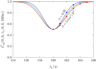
VII Longitudinal, Lateral, and Temperature Effects on Antibunching

The normalized two-particle distribution function $\bar{C}_{\text{st}}(\bar{\bm{r}}_{1},\bar{\bm{r}}_{2})$, evaluated on the basis of the expressions (48) and (54), is shown in Figs. 2–4. The two-particle distribution (the number of coincidence counts) is always suppressed when the two detectors are close together. The dips in the figures represent antibunching.

It is clear from the expression (28) for the two-particle distribution that the number of coincidences is reduced to one half of that naively expected on the basis of the counts by the single detectors, when the two (ideal) point detectors are at the same point. This is understood by the expression (32): the triplet spin states accompany the antisymmetric wave function in space, yielding antibunching, while the singlet spin state accompanies the symmetric wave function in space, yielding bunching. The interplay of these contributions (three fourths from the antibunching and one fourth from bunching) results in the minimum value $0.5\,(=1-3/4+1/4)$ of the normalized two-particle distribution function. The width of the dip, on the other hand, is governed by the width of the spectrum of the emitted particles, as is clear from the analytical formula (56) or from the Fourier-integral representation of the interference term in (38).

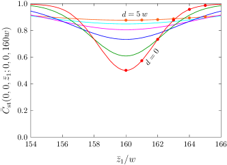
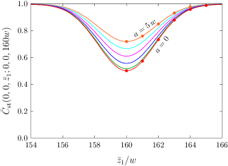
Let us next look at the effects of the detector resolutions. Not only the longitudinal resolution of the detectors $d$ (Fig. 2) but also the lateral size of the detectors $a$ affects the visibility of the antibunching (Fig. 3), although we are looking at the coincidences between the two detectors located along the longitudinal axis. The width of the dip is broadened by the longitudinal resolution of the detectors $d$, while it is not by the lateral size $a$.

The analytical formula (56) clearly reveals how the resolutions of the detectors affect the coincidence counts. It also shows that the detectors can be regarded as point detectors when

$$a\ll\frac{\bar{z}}{\sqrt{2}\,wk_{0}},\qquad d\ll\frac{1}{2\,\delta k_{z}},$$ (76)

and these quantities characterize the lateral and longitudinal coherence lengths, respectively. Clearly, the above conditions agree with those derived in classical textbooks MandelWolf .

The temperature of the source affects antibunching in a way that deserves a few words of explanation. The visibility (namely, the depth of the dip) is temperature independent, as a consequence of the antisymmetry of the fermionic state à la Pauli’s principle: indeed, antisymmetry is exact, both for pure and mixed states, and is preserved even at very high temperatures, where the fermionic state is totally mixed. See Fig. 4(a). This is clear in our formulas and figures: the prefactor $-1/2$ does not depend on any details of the source and the experimental setup. See e.g. Eq. (32): in the second line, irrespectively of the temperature distribution $N(\omega_{k})$, when $|\bm{r}_{1}-\bm{r}_{2}|\to\infty$ the interference term (second term in brackets) goes to zero, while at $\bm{r}_{1}=\bm{r}_{2}$ it equals half of the background term (first term in brackets). On the other hand, the width of the dip depends on temperature and even strongly by the location of the monochromator window with respect to the Fermi level, as can be clearly seen in Fig. 4(b). As a consequence, the dip becomes narrower as temperature is increased and the effects of antibunching becomes more difficult to detect.

VIII Application to experiments

It is useful to summarize the meaning of our analysis. Equations (27) and (28) yield the one- and two-particle distributions in the beam, that are expressed in terms of the fermionic operators. Equations (17) and (32) then express these quantities in terms of the “wave functions” $\hat{\varphi}_{\bm{k}}(\bm{r})$ and of the temperature dependent function $N(\omega_{k})$. If the Fermi distribution is plugged in, all formulas apply to fermions: otherwise the analysis in Secs. IV–VII is general (modulo some sign changes) and can be applied to bosons as well.

It is interesting to apply our final result (56) to some interesting experimental situations. It is necessary to stress that our analysis is strictly valid only for experiments such that the beam of emitted particles travels in vacuum. If this situation closely resembles the experimental one, then our equations apply; otherwise, additional care is required in order to explain the experimental data. In some experiments, like those in which correlation in the current intensities are observed electron1 ; electron2 , our formulas cannot be applied and a different analysis is required inprep .

Let us start from an analysis of the electron experiment electron3 . One infers the values $a\simeq 2\,\text{mm}$, $w\simeq 18\,\text{nm}$, $k_{0}\simeq 10^{11}\,\text{m}^{-1}$, $z\simeq 10\,\text{cm}$. By plugging these values in Eq. (56), one sees that the first of the two factors multiplying the exponential is of order $10^{-4}$. Moreover, the coherence time is $\Delta t_{\text{coh}}\simeq 32\,\text{fs}$, while the response time of the detectors $\Delta t_{\text{det}}\simeq 26\,\text{ps}$, which yield a value $\simeq 1/300$ for the second factor in front of the exponential. The global factor multiplying the exponential is therefore of order $10^{-6}$, which makes the observation of the phenomenon quite complicated. Indeed, the authors had to apply a lateral magnification technique (nominally of order $\gtrsim 10^{4}$) in order to observe antibunching. Notice also that in our formulas the Coulomb repulsion is neglected. This is a delicate issue that would require additional investigation.

Let us now look at the neutron experiment IOSFP . The relevant values are $a\simeq 1\,\text{cm}$, $w\simeq 1\,\text{cm}$ (a mosaic crystal was used in order to reflect the beam into the apparatus), $k_{0}\simeq 10^{10}\,\text{m}^{-1}$, $z\simeq 10\,\text{m}$. The beam coming out of an oven travels in waveguides for about $100\,\text{m}$, is then monochromatized through back scattering by a prefect crystal and illuminates the whole mosaic crystal on a region of order few $\text{cm}^{2}$, the back reflection being coherent only on regions of order $\simeq\mu\text{m}^{2}$ that are uniformly distributed in the whole volume. By plugging the numerical values of the parameters in Eq. (56), the first factor is of order $10^{-10}$. Moreover, by comparing the coherence time of the neutron wave packet $\Delta t_{\text{coh}}\simeq 20\,\text{ns}$ with the response times of the detectors $\Delta t_{\text{det}}\simeq 0.1\,\mu\text{s}$ (two different types of detectors were used, with response times that differ by a factor 10–20), one obtains a second factor of order $\gtrsim 10^{-1}$ (or smaller by a factor 10 for the other type of detectors), yielding a very small antibunching dip. It is interesting to observe that if we take $w\simeq 1\,\mu\text{m}$ (the size of a monocrystal in the mosaic), by Eq. (56) the first factor is of order $10^{-2}$, the second factor remains identical and one obtains an antibunching dip of a few percent, which can be brought to light by deconvolution and is in agreement with the experimental data. An exhaustive analysis of the physical effects of the mosaic crystal used in back reflection is involved and will be presented elsewhere.

Figure 2: (Color online) Normalized two-particle distribution function $\bar{C}_{\text{st}}(0,0,\bar{z}_{1};0,0,160w)$ vs the longitudinal detector coordinate $\bar{z}_{1}$. $\bar{C}_{\text{st}}$ is evaluated in the stationary state on the basis of the expressions (48) and (54), with the Gaussian detectors located at $\bar{\bm{r}}_{1}=(0,0,\bar{z}_{1})$ and $\bar{\bm{r}}_{2}=(0,0,160w)$. We focus here on the effect of the longitudinal resolution of the detector, $d$. The parameters are $k_{0}=20\,w^{-1}$, $\delta k_{z}=0.5\,w^{-1}$, $a=0$, and from bottom to top (in the dip) $d/w={\color[rgb]{1,0,0}0},{\color[rgb]{0,0.5,0}1},{\color[rgb]{0,0,1}2},{\color[rgb]{1,0,1}3},{\color[rgb]{0,1,1}4},{\color[rgb]{0,0,0}5}$ (in units $\hbar=1$ and $m=1$). We set $\beta=5\,mw^{2}/\hbar^{2}$ (a low temperature) and the Fermi level $\mu=(k_{0}+\delta k_{z})^{2}/2m\simeq 210\,\hbar^{2}/mw^{2}$ (just above the momentum window). Note that in this case $p\simeq 400$ in (43) and the condition (49) imposes $w_{z}\ll 20\,w$. The values based on the numerical integrations of (41) and (51) without the Gaussian approximation are also shown by dots for $d={\color[rgb]{1,0,0}0}$ and ${\color[rgb]{0,0,0}5}\,w$. These were checked to be independent of $w_{z}$ for small $w_{z}$.

(a)	(b)

Figure 3: (Color online) (a) Same as in Fig. 2 but with $d=0$ and from bottom to top $a/w={\color[rgb]{1,0,0}0},{\color[rgb]{0,0.5,0}1},{\color[rgb]{0,0,1}2},{\color[rgb]{1,0,1}3},{\color[rgb]{0,1,1}4},{\color[rgb]{0,0,0}5}$. We study here the effect of the lateral size of the detector, $a$. Note that $p\simeq 225$ for $a={\color[rgb]{0,0,0}5}\,w$ in (43) and the condition (49) imposes $w_{z}\ll 11\,w$. The values based on the numerical integrations of (41) and (51) without the Gaussian approximation are also shown by dots for $a={\color[rgb]{1,0,0}0}$ and ${\color[rgb]{0,0,0}5}\,w$ and were checked to be independent of $w_{z}$ for small $w_{z}$. 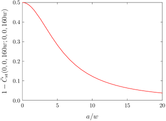(b) Depth of the antibunching dip, $1-\bar{C}_{\text{st}}(0,0,160w;0,0,160w)$, as a function of $a$. All the parameters are the same as in (a).

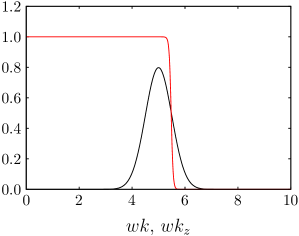
(a)	(b)

Figure 4: (Color online) (a) Same as in Fig. 2 but with $a=0$, $d=0$, and from bottom to top $\beta/(mw^{2}/\hbar^{2})={\color[rgb]{1,0,0}5},{\color[rgb]{0,0.5,0}0.2},{\color[rgb]{0,0,1}0.05}$. We analyze here the effect of the temperature, $\beta^{-1}$. The values based on the numerical integrations of (41) and (51) without the Gaussian approximation are also shown for $\beta/(mw^{2}/\hbar^{2})={\color[rgb]{1,0,0}5}$ and ${\color[rgb]{0,0,1}0.05}$ by dots, and were checked to be independent of $w_{z}$ for small $w_{z}$. (b) Particle emission (from the oven into the beam) is proportional to the overlap of the form factor of the monochromator (bell-shaped curve) and the Fermi distribution function in the oven (step-like function). The effective width of the overlap is inversely proportional to the width of the (antibunching) dip in (a).

Another interesting experiment is that performed with X-rays SPring8 . An important part of this experiment is devoted to the analysis of the lateral coherence features of the beam. The setup involves the values $k_{0}\simeq 7\cdot 10^{10}\,\text{m}^{-1}$, $z\simeq 70\,\text{m}$, while the detector size was changed in the range $a\simeq 10$–$400\,\mu\text{m}$. The authors observed a reduction of the bunching peak very similar to that described in our Fig. 3(b), as a function of the size of the detector mouth $a$, and estimated the lateral coherence length of the beam from the width of the plot, obtaining a source size of order $w\simeq 20\,\mu\text{m}$. The longitudinal coherence length is known to be $\Delta\ell_{\text{coh}}\simeq 2\,\text{mm}$, while the length of the photon bunch is $\Delta\ell_{\text{det}}\simeq 5\,\text{mm}$: by plugging these values in our Eq. (56), the first factor is $\simeq 0.9$ for $a\simeq 10\,\mu\text{m}$, while the second one is $\simeq 0.4$, so that $(1/2)\cdot 0.4\cdot 0.9\simeq 0.18$, which explain well the observed data (a positive bump $\simeq 0.25$.)

Finally, it is interesting to look at some experiments done with thermal optical photon, in order to study both their correlations and imaging. Experiments of this kind were widely debated during the last few years como ; UMBC ; thermalcontrov ; sergienko . We shall focus on the experiment examplethermal , in which the source is a He-Ne laser (in other similar experiments a green-doubled Nd:YAG laser was used). One estimates $a\simeq 30\,\mu\text{m}$, $w\simeq 1\,\text{mm}$, $k_{0}\simeq 10^{7}\,\text{m}^{-1}$, $z\simeq 150\,\text{mm}$. The pseudothermal source is obtained by randomizing the phase of the photon field by means of a rotating ground-glass disk (so that the expression random source would probably be more appropriate). The first factor in Eq. (56) is therefore $\simeq 0.1$ while the second one is essentially 1 ($\Delta t_{\text{det}}\simeq 500\,\text{ps}$, yielding $\Delta\ell_{\text{det}}\simeq 0.15\,\text{m}$, which is to be compared to the much larger coherence length of the laser). This yields an overall dip of good visibility. Unfortunately a quantitative comparison with the experimental data is difficult because the authors, being interested in the change of the width of the second order correlation function with the source size, only plotted a (re)normalized correlation function.

This brief summary of experimental data shows that our analysis and final formulas agree well with most experiments performed so far, with different particles. In some cases a comparison is more complicated and/or requires additional information. One phenomenon that we find of interest, but still lacks experimental confirmation, is our prediction that for fermionic systems we expect that the visibility of second-order interference effects should show no dependence on temperature, as explained in Fig. 4. We emphasized at the end of Sec. VII that this is due to the exactness of Pauli’s principle (yielding perfect antisymmetrization) even for mixed states.

IX Conclusions, Comments, and Perspectives

We analyzed antibunching in a beam of non-interacting fermions and investigated the behavior of the visibility as a function of the size of the source and the detectors, as well as the temperature of the source. These parameters are critical and play a prominent role in experimental applications. Our analysis makes use of Gaussian functions both for the emitting region of the source and the detector, and is adapted to an approximately cylindrically symmetric situation, with circular detector placed close to the longitudinal axis. This is the relevant situation in most experiments, in particular with neutrons and electrons (where however additional Coulomb effects, as well as more specific emission features of the source need to be scrutinized). It is also worth noticing that in the observation of pion correlations CERN the experimental data have been exploited to determine the dimension and the expansion dynamics of the pion “source” (fireball produced in central Pb-Pb collisions, which is expected to be a droplet of quark gluon plasma at the freeze-out point). Clearly, our approach can prove to be quite useful in such a situation as well, when source size and temperature are not known.

Let us look at possible applications and future perspectives. First of all, we emphasize that although our analysis was performed for fermions, all formulas can be easily translated to the case of bosons, enabling one to scrutinize interesting novel experiments in quantum imaging and lithography. Some recent applications make use of chaotic or pseudo-thermal light sources, to which our formalism immediately applies como ; UMBC ; litho .

Other possible applications are in solid state physics, where, as a consequences of the symmetrization procedure of the many-body wave function, entanglement should be present in bulk matter, raising delicate problems in relation to its detection and extraction vedral ; dechiara ; Giovannetti2 . Since one should get entangled neutron pairs within the coherence volume of the wave packet (antibunching being observed within the same coherence volume), these pairs could be used as very efficient “probes” for entanglement in solids in future experiments. This is clearly relevant for quantum information processing and for tests of the Bell inequalities.

Finally, we mention some interesting speculations in neutrino physics and the structure of the universe, where, as a consequence of entanglement formation, the hypothesis of a collisionless fluid of classical point particles can be critically re-examined, yielding a “quantum overpressure,” with significant consequences during the non-linear structure formation epoch at low redshifts neutrino . It is remarkable that independent ideas can bear consequences in very diverse fields.

Appendix A $G(t)$ in the Weak-Coupling Regime

Let us prove (15). We write the matrix (13b) as

$$\hat{G}^{-1}(s)=\hat{D}(s)+\lambda^{2}\hat{K}(s),\qquad\hat{D}_{\bm{k}\bm{k}^{\prime}}(s)=(s+\text{i}\varepsilon_{k})\delta^{3}(\bm{k}-\bm{k}^{\prime}).$$ (77)

Let us show that

$$[1+\lambda^{2}\hat{K}(s)\hat{D}^{-1}(s)]^{-1}$$ (78)

does not have poles in the weak-coupling regime, i.e.

$$\mathop{\text{Det}}\nolimits[1+\lambda^{2}\hat{K}(s)\hat{D}^{-1}(s)]\neq 0,$$ (79)

for a sufficiently small $\lambda$. Indeed, the determinant is evaluated as

$$\mathop{\text{Det}}\nolimits[1+\lambda^{2}\hat{K}(s)\hat{D}^{-1}(s)] =\text{e}^{\mathop{\text{Tr}}\nolimits\log[1+\lambda^{2}\hat{K}(s)\hat{D}^{-1}(s)]},$$ (80)

which reads, in the weak-coupling regime,

$$=1+\lambda^{2}\mathop{\text{Tr}}\nolimits[\hat{K}(s)\hat{D}^{-1}(s)]+O(\lambda^{4})$$

$$=1+\lambda^{2}\int\text{d}^{3}\bm{k}\,\frac{\hat{K}_{\bm{k}\bm{k}}(s)}{s+\text{i}\varepsilon_{k}}+O(\lambda^{4})$$

$$=1+\lambda^{2}\int\text{d}^{3}\bm{k}\int\text{d}^{3}\bm{k}^{\prime}\,\frac{|T_{\bm{k}\bm{k}^{\prime}}|^{2}}{(s+\text{i}\varepsilon_{k})(s+\text{i}\omega_{k^{\prime}})}+O(\lambda^{4}).$$ (81)

Let us look for a zero of the determinant on the first Riemannian sheet, by putting $s=-\text{i}\omega-\gamma/2$:

$$\mathop{\text{Det}}\nolimits[1+\lambda^{2}(\hat{K}\hat{D}^{-1})(-\text{i}\omega-\gamma/2)]=1-\lambda^{2}\int\text{d}^{3}\bm{k}\int\text{d}^{3}\bm{k}^{\prime}\,\frac{|T_{\bm{k}\bm{k}^{\prime}}|^{2}}{(\varepsilon_{k}-\omega+\text{i}\gamma/2)(\omega_{k^{\prime}}-\omega+\text{i}\gamma/2)}+O(\lambda^{4}).$$ (82)

Assume now that the square of the emission matrix in the energy representation,

$$\Gamma(\omega,\omega^{\prime})=(2\pi)^{2}\int\text{d}^{3}\bm{k}\int\text{d}^{3}\bm{k}^{\prime}\,|T_{\bm{k}\bm{k}^{\prime}}|^{2}\delta(\varepsilon_{k}-\omega)\delta(\omega_{k^{\prime}}-\omega^{\prime}),$$ (83)

does not contain any “nonlocal” part $\delta(\omega-\omega^{\prime})$ and has the properties

$$\Gamma(\omega,\omega^{\prime})\to 0\quad\text{for}\quad\omega,\omega^{\prime}\to 0,\infty$$ (84)

[assuming some good continuity property for $\Gamma(\omega,\omega^{\prime})$]. For such a “reasonable” emission matrix $T_{\bm{k}\bm{k}^{\prime}}$, the integral in the second term of (83)

$$\int_{0}^{\infty}\frac{\text{d}\omega_{1}}{2\pi}\int_{0}^{\infty}\frac{\text{d}\omega_{2}}{2\pi}\frac{\Gamma(\omega_{1},\omega_{2})}{(\omega_{1}-\omega+\text{i}\gamma/2)(\omega_{2}-\omega+\text{i}\gamma/2)}$$ (85)

is convergent for any $\omega$ and $\gamma$, and the determinant can always be made non-zero by choosing a sufficiently small $\lambda$. The pole of

$$\hat{G}(s)=\hat{D}^{-1}(s)[1+\lambda^{2}\hat{K}(s)\hat{D}^{-1}(s)]^{-1},$$ (86)

therefore, comes from the first factor $\hat{D}_{\bm{k}\bm{k}^{\prime}}^{-1}(s)$, i.e. $s_{\text{pole}}=-\text{i}\varepsilon_{k}$, and we are allowed to expand the nonsingular second factor as a power series of $\lambda$, yielding

$$G_{\bm{k}\bm{k}^{\prime}}(t)=\delta^{3}(\bm{k}-\bm{k}^{\prime})\text{e}^{-\text{i}\varepsilon_{k}t}+O(\lambda^{2}).$$ (87)

Appendix B Two-Particle Distribution in a Noncollinear Arrangement

Here we briefly sketch the derivation of (71). Remembering

$$\bar{\bm{r}}_{1}=(\bar{r}_{1}\sin\Theta_{\text{d}}\cos\Phi,\bar{r}_{1}\sin\Theta_{\text{d}}\sin\Phi,\bar{r}_{1}\cos\Theta_{\text{d}}),$$ (88a)

$$\bar{\bm{r}}_{2}=(-\bar{r}_{2}\sin\Theta_{\text{d}}\cos\Phi,-\bar{r}_{2}\sin\Theta_{\text{d}}\sin\Phi,\bar{r}_{2}\cos\Theta_{\text{d}}),$$ (88b)

the functions $\mathcal{Z}_{k_{1}k_{2}}(\bar{\bm{r}})$ and $\mathcal{A}_{\bm{k}_{1}\bm{k}_{2}}(\bar{\bm{r}})$ read

$$\mathcal{Z}_{k_{1}k_{2}}(\bar{\bm{r}})=\theta(k_{1z})f(k_{1}\hat{\bar{\bm{r}}})\theta(k_{2z})f(k_{2}\hat{\bar{\bm{r}}})\text{e}^{-(k_{1}-k_{2})^{2}\hat{\bar{\bm{r}}}\cdot\mathcal{D}^{2}\hat{\bar{\bm{r}}}/2},$$ (89a)

$$\mathcal{A}_{\bm{k}_{1}\bm{k}_{2}}(\bar{\bm{r}})=\frac{m^{2}}{(2\pi)^{5}}\text{e}^{-(\Delta\bm{k}_{1\hat{\bar{\bm{r}}}}\cdot\mathcal{W}^{2}\Delta\bm{k}_{1\hat{\bar{\bm{r}}}}+\Delta\bm{k}_{2\hat{\bar{\bm{r}}}}\cdot\mathcal{W}^{2}\Delta\bm{k}_{2\hat{\bar{\bm{r}}}})/2}.$$ (89b)

By substituting (89) into (37) and (38) and introducing spherical coordinates, we get

$$\bar{\rho}_{\text{st}}(\bar{\bm{r}})=\lambda^{2}\frac{2m^{2}}{(2\pi)^{5}\bar{r}^{2}}\int_{0}^{\infty}\text{d}k\,k^{2}N(\omega_{k})f^{2}(k\hat{\bar{\bm{r}}})\int_{0}^{\pi/2}\text{d}\theta\sin\theta\int_{0}^{2\pi}\text{d}\phi\,\text{e}^{-\Delta\bm{k}_{\hat{\bar{\bm{r}}}}\cdot\mathcal{W}^{2}\Delta\bm{k}_{\hat{\bar{\bm{r}}}}},$$ (90)

$$\bar{\mathcal{I}}_{\text{st}}(\bar{\bm{r}}_{1},\bar{\bm{r}}_{2})=\lambda^{4}\frac{2m^{4}}{(2\pi)^{10}\bar{r}_{1}^{2}\bar{r}_{2}^{2}}\int_{0}^{\infty}\text{d}k_{1}\,k_{1}^{2}\int_{0}^{\infty}\text{d}k_{2}\,k_{2}^{2}N(\omega_{k_{1}})N(\omega_{k_{2}})f(k_{1}\hat{\bar{\bm{r}}}_{1})f(k_{2}\hat{\bar{\bm{r}}}_{1})f(k_{1}\hat{\bar{\bm{r}}}_{2})f(k_{2}\hat{\bar{\bm{r}}}_{2})\\ {}\times\text{e}^{-\text{i}(k_{1}-k_{2})(\bar{r}_{1}-\bar{r}_{2})}\text{e}^{-(k_{1}-k_{2})^{2}(\hat{\bar{\bm{r}}}_{1}\cdot\mathcal{D}^{2}\hat{\bar{\bm{r}}}_{1}+\hat{\bar{\bm{r}}}_{2}\cdot\mathcal{D}^{2}\hat{\bar{\bm{r}}}_{2})/2}J(k_{1};\bar{\bm{r}}_{1},\bar{\bm{r}}_{2})J(k_{2};\bar{\bm{r}}_{1},\bar{\bm{r}}_{2}),$$ (91)

where

$$J(k;\bar{\bm{r}}_{1},\bar{\bm{r}}_{2})=\int_{0}^{\pi/2}\text{d}\theta\sin\theta\int_{0}^{2\pi}\text{d}\phi\,\text{e}^{-(\Delta\bm{k}_{\hat{\bar{\bm{r}}}_{1}}\cdot\mathcal{W}^{2}\Delta\bm{k}_{\hat{\bar{\bm{r}}}_{1}}+\Delta\bm{k}_{\hat{\bar{\bm{r}}}_{2}}\cdot\mathcal{W}^{2}\Delta\bm{k}_{\hat{\bar{\bm{r}}}_{2}})/2}.$$ (92)

Note that, when $\hat{\bar{\bm{r}}}_{1}$ and $\hat{\bar{\bm{r}}}_{2}$ satisfy (88), one has

$$f(k\hat{\bar{\bm{r}}}_{1})=f(k\hat{\bar{\bm{r}}}_{2})=\frac{1}{[(2\pi)^{3}(\delta k_{z})^{2}(\delta k_{\perp})^{4}]^{1/4}}\exp\!\left(-\frac{k^{2}\sin^{2}\!\Theta_{\text{d}}}{4(\delta k_{\perp})^{2}}-\frac{(k\cos\Theta_{\text{d}}-k_{0})^{2}}{4(\delta k_{z})^{2}}\right)\equiv f(k,\Theta_{\text{d}}),$$ (93)

and $\hat{\bar{\bm{r}}}_{1}\cdot\mathcal{D}^{2}\hat{\bar{\bm{r}}}_{1}=\hat{\bar{\bm{r}}}_{2}\cdot\mathcal{D}^{2}\hat{\bar{\bm{r}}}_{2}=a^{2}\sin^{2}\!\Theta_{\text{d}}+d^{2}\cos^{2}\!\Theta_{\text{d}}$.

B.1 First-Order Correlation

Let us first consider the case where $\bm{r}=\bm{r}_{1}$. Since

$$\Delta\bm{k}_{\hat{\bar{\bm{r}}}}\cdot\mathcal{W}^{2}\Delta\bm{k}_{\hat{\bar{\bm{r}}}}=w^{2}k^{2}(\sin^{2}\!\Theta_{\text{d}}+\sin^{2}\!\theta)+w_{z}^{2}k^{2}(\cos\Theta_{\text{d}}-\cos\theta)^{2}-2w^{2}k^{2}\sin\Theta_{\text{d}}\sin\theta\cos(\Phi-\phi),$$ (94)

one has

$$\int_{0}^{\pi/2}\text{d}\theta\sin\theta\int_{0}^{2\pi}\text{d}\phi\,\text{e}^{-\Delta\bm{k}_{\hat{\bar{\bm{r}}}}\cdot\mathcal{W}^{2}\Delta\bm{k}_{\hat{\bar{\bm{r}}}}}=\text{e}^{-p\sin^{2}\!\Theta_{\text{d}}}\int_{0}^{\pi/2}\text{d}\theta\sin\theta\,\text{e}^{-p\sin^{2}\!\theta-q(\cos\Theta_{\text{d}}-\cos\theta)^{2}}\int_{0}^{2\pi}\text{d}\phi\,\text{e}^{2p\sin\Theta_{\text{d}}\sin\theta\cos(\Phi-\phi)},$$ (95)

where $p=w^{2}k^{2}$ and $q=w_{z}^{2}k^{2}$. The integral over $\phi$ yields a modified Bessel function of the first kind:

$$\int_{0}^{2\pi}\text{d}\phi\,\text{e}^{2p\sin\Theta_{\text{d}}\sin\theta\cos(\Phi-\phi)}=2\pi I_{0}(2p\sin\Theta_{\text{d}}\sin\theta)=2\pi\sum_{m=0}^{\infty}\frac{(p\sin\Theta_{\text{d}}\sin\theta)^{2m}}{(m!)^{2}}.$$ (96)

Therefore, with the aid of the trick used in (54), we have

$$\int_{0}^{\pi/2}\text{d}\theta\sin\theta\int_{0}^{2\pi}\text{d}\phi\,\text{e}^{-\Delta\bm{k}_{\hat{\bar{\bm{r}}}}\cdot\mathcal{W}^{2}\Delta\bm{k}_{\hat{\bar{\bm{r}}}}}$$

$$\qquad\qquad=2\pi\text{e}^{-p\sin^{2}\!\Theta_{\text{d}}}\sum_{m=0}^{\infty}\frac{(p^{2}\sin^{2}\!\Theta_{\text{d}})^{m}}{(m!)^{2}}\int_{0}^{\pi/2}\text{d}\theta\sin^{2m+1}\!\theta\,\text{e}^{-p\sin^{2}\!\theta-q(\cos\Theta_{\text{d}}-\cos\theta)^{2}}$$

$$\qquad\qquad=2\pi\text{e}^{-p\sin^{2}\!\Theta_{\text{d}}}\sum_{m=0}^{\infty}\frac{(p^{2}\sin^{2}\!\Theta_{\text{d}})^{m}}{(m!)^{2}}\left(-\frac{\partial}{\partial p}\right)^{m}\int_{0}^{\pi/2}\text{d}\theta\sin\theta\,\text{e}^{-p\sin^{2}\!\theta-q(\cos\Theta_{\text{d}}-\cos\theta)^{2}}.$$ (97)

Hereafter, the integral over $\theta$ is evaluated when $p\gg q$ and $p\gg 1$. By changing the integration variable, we have

$$\int_{0}^{\pi/2}\text{d}\theta\sin\theta\,\text{e}^{-p\sin^{2}\!\theta-q(\cos\Theta_{\text{d}}-\cos\theta)^{2}}=\frac{\text{e}^{-p\left(1+\frac{q\cos^{2}\!\Theta_{\text{d}}}{p-q}\right)}}{\sqrt{p-q}}\,\Biggl{(}\int_{\frac{q\cos\Theta_{\text{d}}}{\sqrt{p-q}}}^{1}\text{d}x\,\text{e}^{x^{2}}+\int_{1}^{\sqrt{p-q}+\frac{q\cos\Theta_{\text{d}}}{\sqrt{p-q}}}\text{d}x\,\text{e}^{x^{2}}\Biggr{)}.$$ (98)

The first term is of order of $\text{e}^{-p}/\sqrt{p}$. Integrating by parts, the second term becomes

$$\frac{\text{e}^{-p\left(1+\frac{q\cos^{2}\!\Theta_{\text{d}}}{p-q}\right)}}{\sqrt{p-q}}\int_{1}^{\sqrt{p-q}+\frac{q\cos\Theta_{\text{d}}}{\sqrt{p-q}}}\text{d}x\,\text{e}^{x^{2}}=\frac{\text{e}^{-q(\cos\Theta_{\text{d}}-1)^{2}}}{2(p-q+q\cos\Theta_{\text{d}})}\left(1+\frac{1}{2\left(\sqrt{p-q}+\frac{q\cos\Theta_{\text{d}}}{\sqrt{p-q}}\right)^{2}}\right)\\ -\frac{3\text{e}}{4}\frac{\text{e}^{-p\left(1+\frac{q\cos^{2}\!\Theta_{\text{d}}}{p-q}\right)}}{\sqrt{p-q}}{}+\frac{\text{e}^{-p\left(1+\frac{q\cos^{2}\!\Theta_{\text{d}}}{p-q}\right)}}{\sqrt{p-q}}\int_{1}^{\sqrt{p-q}+\frac{q\cos\Theta_{\text{d}}}{\sqrt{p-q}}}\text{d}x\,\frac{3\text{e}^{x^{2}}}{4x^{4}},$$ (99)

where the second and third terms are, respectively, $O(1/p^{3/2})$ and $O(\text{e}^{-p}/\sqrt{p})$, and the last term can be shown to be O$(p^{-5/4})$. Thus, one has

$$\int_{0}^{\pi/2}\text{d}\theta\sin\theta\,\text{e}^{-p\sin^{2}\!\theta-q(\cos\Theta_{\text{d}}-\cos\theta)^{2}} =\frac{\text{e}^{-q(\cos\Theta_{\text{d}}-1)^{2}}}{2(p-q+q\cos\Theta_{\text{d}})}+O(p^{-{5/4}})$$

$$=\frac{\text{e}^{-q(\cos\Theta_{\text{d}}-1)^{2}}}{2p}+O(p^{-{5/4}}).$$ (100)

By substituting (100) into (97) and retaining the leading order terms in $1/p$, we have

$$\int_{0}^{\pi/2}\text{d}\theta\sin\theta\int_{0}^{2\pi}\text{d}\phi\,\text{e}^{-\Delta\bm{k}_{\hat{\bar{\bm{r}}}}\cdot\mathcal{W}^{2}\Delta\bm{k}_{\hat{\bar{\bm{r}}}}} =2\pi\text{e}^{-p\sin^{2}\!\Theta_{\text{d}}}\sum_{m=0}^{\infty}\frac{(p^{2}\sin^{2}\!\Theta_{\text{d}})^{m}}{(m!)^{2}}\left(-\frac{\partial}{\partial p}\right)^{m}\frac{\text{e}^{-q(\cos\Theta_{\text{d}}-1)^{2}}}{2p}$$

$$=\pi\text{e}^{-p\sin^{2}\!\Theta_{\text{d}}}\text{e}^{-q(\cos\Theta_{\text{d}}-1)^{2}}\sum_{m=0}^{\infty}\frac{(p^{2}\sin^{2}\!\Theta_{\text{d}})^{m}}{(m!)^{2}}\frac{m!}{p^{m+1}}$$

$$=\frac{\pi}{p}\text{e}^{-p\sin^{2}\!\Theta_{\text{d}}-q(1-\cos\Theta_{\text{d}})^{2}}\text{e}^{p\sin^{2}\!\Theta_{\text{d}}}$$

$$=\frac{\pi}{w^{2}k^{2}}\text{e}^{-w_{z}^{2}k^{2}(1-\cos\Theta_{\text{d}})^{2}}.$$ (101)

Then, the one-particle correlation is

$$\bar{\rho}_{\text{st}}(\bar{\bm{r}})=\lambda^{2}\frac{m^{2}}{(2\pi)^{4}w^{2}\bar{r}^{2}}\int_{0}^{\infty}\text{d}k\,N(\omega_{k})f^{2}(k,\Theta_{\text{d}})\text{e}^{-w_{z}^{2}k^{2}(1-\cos\Theta_{\text{d}})^{2}}.$$ (102)

When $\bar{\bm{r}}=\bar{\bm{r}}_{2}$, we obtain the same result. This is the denominator of Eqs. (29) and (71).

B.2 Second-Order Correlation

Because (88) leads to

$$\frac{1}{2}(\Delta\bm{k}_{\hat{\bar{\bm{r}}}_{1}}\cdot\mathcal{W}^{2}\Delta\bm{k}_{\hat{\bar{\bm{r}}}_{1}}+\Delta\bm{k}_{\hat{\bar{\bm{r}}}_{2}}\cdot\mathcal{W}^{2}\Delta\bm{k}_{\hat{\bar{\bm{r}}}_{2}})=p(\sin^{2}\!\Theta_{\text{d}}+\sin^{2}\!\theta)+q(\cos\Theta_{\text{d}}-\cos\theta)^{2},$$ (103)

the auxiliary function $J(k;\bar{\bm{r}}_{1},\bar{\bm{r}}_{2})$ is evaluated as

$$J(k;\bar{\bm{r}}_{1},\bar{\bm{r}}_{2}) =2\pi\int_{0}^{\pi/2}\text{d}\theta\sin\theta\,\text{e}^{-p(\sin^{2}\!\Theta_{\text{d}}+\sin^{2}\!\theta)-q(\cos\Theta_{\text{d}}-\cos\theta)^{2}}$$

$$=\frac{\pi}{w^{2}k^{2}}\text{e}^{-w^{2}k^{2}\sin^{2}\!\Theta_{\text{d}}}\text{e}^{-w_{z}^{2}k^{2}(1-\cos\Theta_{\text{d}})^{2}},$$ (104)

where we have used (100) in the second equality. Thus, in terms of $f(k_{j},\Theta_{\text{d}})$ ($j=1,2$),

$$\bar{\mathcal{I}}_{\text{st}}(\bar{\bm{r}}_{1},\bar{\bm{r}}_{2})=\lambda^{4}\frac{m^{4}}{2(2\pi)^{8}w^{4}\bar{r}_{1}^{2}\bar{r}_{2}^{2}}\int_{0}^{\infty}\text{d}k_{1}\int_{0}^{\infty}\text{d}k_{2}\,N(\omega_{k_{1}})N(\omega_{k_{2}})f^{2}(k_{1},\Theta_{\text{d}})f^{2}(k_{2},\Theta_{\text{d}})\text{e}^{-\text{i}(k_{1}-k_{2})(\bar{r}_{1}-\bar{r}_{2})}\\ {}\times\text{e}^{-(k_{1}-k_{2})^{2}(a^{2}\sin^{2}\!\Theta_{\text{d}}+d^{2}\cos^{2}\!\Theta_{\text{d}})}\text{e}^{-(k_{1}^{2}+k_{2}^{2})[w^{2}\sin^{2}\!\Theta_{\text{d}}+w_{z}^{2}(1-\cos\Theta_{\text{d}})^{2}]}.$$ (105)

This is the numerator of Eqs. (29) and (71).

B.3 Well-Monochromatized Case

If the beam of particles is well-monochromatized and the distribution $N(\omega_{k})$ is a slowly varying function there, we have

$$\bar{\rho}_{\text{st}}(\bar{\bm{r}}) =\lambda^{2}\frac{m^{2}}{(2\pi)^{4}w^{2}\bar{r}^{2}}N(\omega_{k_{0}})\int_{-\infty}^{\infty}\text{d}k\,f^{2}(k,\Theta_{\text{d}})\text{e}^{-w_{z}^{2}k^{2}(1-\cos\Theta_{\text{d}})^{2}}$$

$$=\lambda^{2}\frac{m^{2}}{(2\pi)^{5}w^{2}\bar{r}^{2}(\delta k_{\perp})\sqrt{D_{1}(\Theta_{\text{d}})}}N(\omega_{k_{0}})\exp\!\left[-\frac{k_{0}^{2}}{2(\delta k_{z})^{2}}\left(1-\frac{(\delta k_{\perp})^{2}\cos^{2}\!\Theta_{\text{d}}}{D_{1}(\Theta_{\text{d}})}\right)\right],$$ (106)

where the Gaussian $k$-integration has been carried out with the aid of

$$-\frac{k^{2}\sin^{2}\!\Theta_{\text{d}}}{2(\delta k_{\perp})^{2}}-\frac{k^{2}\cos^{2}\!\Theta_{\text{d}}-2k_{0}k\cos\Theta_{\text{d}}+k_{0}^{2}}{2(\delta k_{z})^{2}} -w_{z}^{2}k^{2}(1-\cos\Theta_{\text{d}})^{2}$$

$$=-\frac{D_{1}(\Theta_{\text{d}})}{2(\delta k_{z})^{2}(\delta k_{\perp})^{2}}k^{2}+\frac{k_{0}\cos\Theta_{\text{d}}}{(\delta k_{z})^{2}}k-\frac{k_{0}^{2}}{2(\delta k_{z})^{2}}.$$ (107)

On the other hand, we have

$$\bar{\mathcal{I}}_{\text{st}}(\bar{\bm{r}}_{1},\bar{\bm{r}}_{2})=\lambda^{4}\frac{m^{4}}{2(2\pi)^{8}w^{4}\bar{r}_{1}^{2}\bar{r}_{2}^{2}}N^{2}(\omega_{k_{0}})\int_{-\infty}^{\infty}\text{d}k_{1}\int_{-\infty}^{\infty}\text{d}k_{2}\,f^{2}(k_{1},\Theta_{\text{d}})f^{2}(k_{2},\Theta_{\text{d}})\text{e}^{-\text{i}(k_{1}-k_{2})(\bar{r}_{1}-\bar{r}_{2})}\\ {}\times\text{e}^{-(k_{1}-k_{2})^{2}(a^{2}\sin^{2}\!\Theta_{\text{d}}+d^{2}\cos^{2}\!\Theta_{\text{d}})}\text{e}^{-(k_{1}^{2}+k_{2}^{2})[w^{2}\sin^{2}\!\Theta_{\text{d}}+w_{z}^{2}(1-\cos\Theta_{\text{d}})^{2}]}.$$ (108)

In terms of $K=(k_{1}+k_{2})/2$ and $k=k_{1}-k_{2}$, one has

$$-\sum_{j=1}^{2}\left(\frac{k_{j}^{2}\sin^{2}\!\Theta_{\text{d}}}{2(\delta k_{\perp})^{2}}+\frac{k_{j}^{2}\cos^{2}\!\Theta_{\text{d}}-2k_{0}k_{j}\cos\Theta_{\text{d}}+k_{0}^{2}}{2(\delta k_{z})^{2}}\right)-\text{i}(k_{1}-k_{2})(\bar{r}_{1}-\bar{r}_{2})\\ {}-(k_{1}-k_{2})^{2}(a^{2}\sin^{2}\!\Theta_{\text{d}}+d^{2}\cos^{2}\!\Theta_{\text{d}})-(k_{1}^{2}+k_{2}^{2})[w^{2}\sin^{2}\!\Theta_{\text{d}}+w_{z}^{2}(1-\cos\Theta_{\text{d}})^{2}]\\ =-\frac{D_{2}(\Theta_{\text{d}})}{(\delta k_{z})^{2}(\delta k_{\perp})^{2}}K^{2}+\frac{2k_{0}\cos\Theta_{\text{d}}}{(\delta k_{z})^{2}}K-\frac{k_{0}^{2}}{(\delta k_{z})^{2}}-\frac{D_{3}(\Theta_{\text{d}})}{4(\delta k_{z})^{2}(\delta k_{\perp})^{2}}k^{2}-\text{i}k(\bar{r}_{1}-\bar{r}_{2}),$$ (109)

and, thus,

$$\bar{\mathcal{I}}_{\text{st}}(\bar{\bm{r}}_{1},\bar{\bm{r}}_{2})=\lambda^{4}\frac{m^{4}}{2(2\pi)^{10}w^{4}\bar{r}_{1}^{2}\bar{r}_{2}^{2}(\delta k_{\perp})^{2}\sqrt{D_{2}(\Theta_{\text{d}})D_{3}(\Theta_{\text{d}})}}N^{2}(\omega_{k_{0}})\\ {}\times\exp\!\left[-\frac{k_{0}^{2}}{(\delta k_{z})^{2}}\left(1-\frac{(\delta k_{\perp})^{2}\cos^{2}\!\Theta_{\text{d}}}{D_{2}(\Theta_{\text{d}})}\right)-\frac{(\delta k_{z})^{2}(\delta k_{\perp})^{2}(\bar{r}_{1}-\bar{r}_{2})^{2}}{D_{3}(\Theta_{\text{d}})}\right].$$ (110)

By plugging (102) and (105) into (29), we obtain the normalized two-particle distribution function (71).