A sample of mJy radio sources at 1.4 GHz in the Lynx and Hercules fields - I. Radio imaging, multicolour photometry and spectroscopy

Abstract

With the goal of identifying high redshift radio galaxies with FRI classification, here are presented high resolution, wide–field radio observations, near infra–red and optical imaging and multi–object spectroscopy of two fields of the Leiden–Berkeley Deep Survey. These fields, Hercules.1 and Lynx.2, contain a complete sample of 81 radio sources with S${}_{\rm 1.4GHz}>0.5$ mJy within 0.6 square degrees. This sample will form the basis for a study of the population and cosmic evolution of high redshift, low power, FRI radio sources which will be presented in Paper II. Currently, the host galaxy identification fraction is 86% with 11 sources remaining unidentified at a level of r^′$\geqslant$25.2 mag (Hercules; 4 sources) or r^′$\geqslant$24.4 mag (Lynx; 7 sources) or K$\mathrel{\hbox{\hbox to0.0pt{\hbox{\lower 4.0pt\hbox{$\sim$}}\hss}\hbox{$>$}}}$20 mag. Spectroscopic redshifts have been determined for 49% of the sample and photometric redshift estimates are presented for the remainder of the sample.

1 Introduction

Radio–loud active galaxies that display extended jet emission from their central cores can be divided into two main types; Fanaroff & Riley class I and II (FRI and FRII; Fanaroff & Riley 1974). The galaxies of FRI type are ‘edge–darkened’ with the majority of their emission confined to their central regions and jets that flare out close to the nucleus. On the other hand, the FRII galaxies are ‘edge–brightened’ meaning the bulk of their emission originates from the hotspots at the ends of their highly collimated jets. The FRII galaxies are the more luminous of the two classes and typically have $P_{\rm 178MHz}$ $>10^{24-25}$ WHz^-1sr^-1  but there is significant overlap at the break luminosity. The FRIs and FRIIs have also been suggested as the unbeamed parent populations of BL Lac objects and flat spectrum quasars respectively (Jackson & Wall, 1999).

The differences between the two FR classes are not confined to the lobe morphology. For instance, Zirbel & Baum (1995) found that the FRIIs produce 10–50 times more emission line luminosity than the FRIs at a particular radio core power. Additionally, optical observations by Owen & Laing (1989) found that the host galaxies of FRIs tended to be larger and more luminous than those of FRIIs, though later work by Ledlow & Owen (1996) suggested that this result was caused by a combination of sample selection effect, and only observing a small range in radio power.

It is not yet clear whether the observed morphological differences between the two FR classes are the result of fundamental differences in the properties of the central engine (e.g. lower accretion rates in FRIs leading to advection dominated accretion flow, or a slower FRI black hole spin) as advocated by e.g. Baum et. al. (1995), or differences in the interactions of the jets with their environments as suggested by the work of Gopal–Krishna & Wiita (2000) and Gawroński et al. (2006). This intrinsic/extrinsic question is of vital importance for understanding the relationship between these objects; if the intrinsic difference model is correct then the FRIs and FRIIs are two discrete classes of object, however if the evidence suggests the other model is correct, the underlying properties of the classes would be the same. In the latter case the two classes may simply represent different stages in the evolution of a radio galaxy, i.e. it starts out as a powerful, high–luminosity FRII and as it ages its jets become less powerful and it becomes an FRI (e.g. Willott et al. 2001).

One of the key ways in which the differences between the two classes can be investigated is through their evolution with cosmic epoch since, if the extrinsic model is correct, then FRIs and FRIIs of the same luminosity should evolve in similar ways. FRIIs are known to undergo strong cosmic evolution, with density enhancements for the most luminous of a factor of 100-1000 out to redshifts of 1–2, compared to a factor of $\sim\!\!$ 10 for the less luminous, sources (Wall, 1980); the behaviour of the FRIs is less clear. Low–redshift studies initially suggested that they had a constant space density (e.g. Jackson & Wall 1999; Willott et al. 2001) and this appeared to be confirmed at higher redshift by Clewley & Jarvis (2004). However, they selected the FRIs in their sample using a luminosity cut; this could lead to FRIs being missed (particularly the more luminous FRIs which may evolve the most) since the FRI/FRII break luminosity is not fixed, but is a function of host galaxy magnitude (Ledlow & Owen 1996). It is clear therefore, that to define a robust sample of distant FRIs, in order to obtain an accurate picture of their high redshift behaviour, radio morphological classification is a necessity.

Determining the cosmic evolution of FRI radio galaxies is also important because of the impact that they may have on galaxy formation and evolution. Models of galaxy formation are increasingly turning to these objects to solve the problem of massive galaxy over–growth (e.g. Bower et al., 2006). It is predominantly the lower luminosity sources that provide the necessary feedback for this, (Best et al., 2006), and may possibly be limited to the FRI population alone. As such understanding the little studied FRI sources and their evolution could be critical to deciphering this mechanism.

The first significant attempt at determining the FRI high–redshift space density was carried out by Snellen & Best (2001) using the Hubble Deep Field and Flanking Fields (HDF+FF). Two z$>$1 FRI galaxies were detected in this area, which calculations showed to be broadly consistent with an FRI space density enhancement comparable to that of less luminous FRII galaxies at that redshift, and inconsistent (a probability of $<$1%) with a non-evolving FRI population. However, with only two detected FRIs the uncertainties in this result are clearly large.

The area of sky used in the analysis of Snellen & Best (2001) was only large enough to give a first estimate of the high redshift space density of FRIs. This work, therefore, uses a deep, wide–field, Very Large Array (VLA) A–array survey an order of magnitude larger than the HDF+HFF which will enable the space density to be directly measured for the first time. Here we present the initial radio, optical and infra–red imaging, along with the spectroscopic observations which form the basis of the work. The layout of the paper is as follows: in Sections 2 and 3 the sample is defined and the new radio observations taken are described; in Sections 4 and 5, the optical and infra–red imaging are presented and the host galaxies identified; Sections 6 and 7 describe the spectroscopic observations of a subset of the sample. Finally, Section 8 outlines the redshift estimation methods used for the remainder of the sample and the conclusions of the paper can be found in Section 9.

2 The radio sample

The survey was split over two fields – one in the constellation of Lynx at right ascension, $\alpha=8h45$, declination, $\delta=+44.6\hbox{${}^{\circ}$}$ (J2000) and one in Hercules at $\alpha=17h20$, $\delta=+49.9\hbox{${}^{\circ}$}$ (J2000). These fields were chosen because of the existence of previous low resolution radio observations by Windhorst et al. (1984), Oort & Windhorst (1985) and Oort & van Langevelde (1987). Additionally, the Hercules field has some previous optical and spectroscopic observations by Waddington et al. (2000). Alongside this, the Lynx field is also covered by the Sloan Digital Sky Survey (SDSS; York et al. 2000; Stoughton et al. 2002).

The two fields were originally observed as part of the Leiden–Berkeley Deep Survey (LBDS) in which they were referred to as Lynx.2 and Hercules.1. For the remainder of this paper they will be referred to as Lynx and Hercules respectively. It should be noted that the Lynx.2 field is unusual in that it does not contain any radio sources brighter than 6 mJy over nearly a square degree. However, the resulting underrepresentation in the radio source counts above this level should not affect the conclusions of this paper, as it is the faint end of the RLF that is being investigated here. This section outlines the previous work in the two fields.

2.1 Sample definition and previous radio work

The LBDS survey was constructed to provide photometry for faint galaxies and quasars, via multicolour plates obtained with the 4m Mayall Telescope at Kitt Peak (Kron, 1980; Koo & Kron 1982). Radio follow–up of nine of the LBDS fields (including Hercules and Lynx that are used here) was performed subsequently using the 3km Westerbork Synthesis Radio Telescope (WSRT) at 1.4 GHz, at a resolution of 12.5^′′ (Windhorst et al. 1984), reaching a rms noise level, at the field centre, of 0.12–0.28 mJy. Their radio sample consists of 306 sources which satisfied the sample selection criteria of peak signal to noise ($S_{P}/N$) $\geq 5\sigma$ out to an attenuation factor, $A(r),\leq 5$ (for WSRT this corresponds to a radius of $\leq 0.464\hbox{${}^{\circ}$}$ or $\leq$ 28^′).

The Hercules and Lynx fields were reobserved by Oort & van Langevelde (1987) and Oort & Windhorst (1985) respectively, again using the 3 km WSRT at 1.4 GHz with a 12.5^′′ beam. These two sets of observations were a factor 2–3 deeper than the original Windhorst et al. (1984) ones, reaching a 5$\sigma$ flux limit of 0.45 mJy for Hercules and 0.30 mJy for Lynx at the pointing centre.

The sample used in this work is a subset of the combined Hercules and Lynx sources, as it is limited by the field of view size of the optical imaging described in §4; this is illustrated in Figure 1. A flux limit of 0.5 mJy was also imposed to remove the faintest, most poorly detected sources and provide a more uniform limiting flux density across the two fields. Table 1 gives the flux densities for the Hercules field (Oort & van Langevelde 1987) and Table 2 gives the same for the Lynx field (Oort & Windhorst 1985) for the sources included in this work. Table 3 gives the 1.4 GHz flux densities of sources which were not covered by the optical observations, but were included in the subsequent infra–red imaging; consequently they are not part of the complete sample, but are included here for completeness. These, and other source parameters, were measured by Oort and collaborators using an elliptical Gaussian fitting method in two dimensions.

Figure 1: The distribution of the radio sources in the Lynx and Hercules fields; the labels correspond to the last 3 characters of the source names. The large circle in both plots represents the 0.464^∘ radius of the previous WSRT observations of e.g. Windhorst et al. (1984); this is also approximately the 30^′primary beam of the VLA at 1.4 GHz. The dotted line represents the area of the sample which is defined by the field of view of the optical imaging. Dots indicate the positions of the additional sources which were not included in the sample because they either fell below the flux density limit of 0.5 mJy, or they are not covered by the sample area. Open diamonds indicate sources not included in the complete sample, but which were included in the infra–red observations.

2.2 Sample completeness

The selection criteria of the LBDS meant that source weighting was necessary to account for incompleteness in the starting sample. This incompleteness arises from two factors: the attenuation of the WSRT primary beam and the resolution bias. The effect of the first of these factors, the decreasing sensitivity at increasing radial distance from the pointing centre, is to make the probability of detecting a source depend on where it is located in the map; a source which just satisfies the selection criteria at the centre would have been missed if it was located at the map edge. To correct for this each source was assigned a weight that was inversely proportional to the area over which it would have met the selection criteria and hence, have been included in the sample (Windhorst et al. 1984). The total sample area for the current work is limited by the size of the optical imaging, so the attenuation weights for the sources considered here were recalculated to account for this.

The corrections for the incompleteness due to the resolution bias (the fact that a resolved source will be more difficult to detect than a point source of the same total flux) were found, by Windhorst et al. (1984), through detailed modelling of the source detection algorithms. It was subsequently found that sources with higher flux densities were also those with a large angular size (e.g. Windhorst et al. 1993) which, as Windhorst, Mathis & Neuschaefer (1990) showed, meant that the original weights were overestimated. Waddington et al. (2000) derived a new expression for the resolution bias that took this into account; it is that method which is used in the current calculations.

These two re–derived correction factors, the attenuation weight and resolution weight, were then multiplied together to give the final weights. For further details of the source weighting methods used in the LBDS see Windhorst et al. (1984) and Waddington et al. (2000). See Tables 1 and 2 for the weight calculated for each source.

3 New radio observations

3.1 The observations

The VLA data were taken with the array in A configuration on 22nd April 2002 for the Hercules field, and 15th February 2002 for the Lynx field. Both sets of observations were taken at a frequency of 1.4 GHz (L–band), in four IF spectral line mode to enable wide field imaging, using 16 channels of width 781.25 kHz. The IFs were centred on 1391.3 and 1471.1 MHz observing dual polarization. Both the Hercules and the Lynx fields were observed for 8.5 hours each.

The data were calibrated using the NRAO AIPS package. Because of the non-coplanar geometry of the telescope array, in order to image the entire area of the primary beam, a three–dimensional Fourier transform is required. As this would be computationally impractical, the standard pseudo–three–dimensional Fourier transform technique, as incorporated in the task IMAGR, (Perley 1999) was adopted: this technique divides the field of view into numerous smaller facets, within each of which a two–dimensional Fourier transform provides a sufficiently good approximation. For each of the Hercules and Lynx fields, 256 by 256 pixel facets (with 0.35^′′ per pixel) were centred on all the sources that were already known from the imaging of Windhorst, Oort and collaborators, discussed above. These sub-fields were cleaned and self-calibrated using the AIPS tasks IMAGR and CALIB. The self calibration consisted of multiple phase–only cycles followed by one final amplitude and phase calibration. The resulting maps have a resolution of 1.6^′′  and reach a noise limit of 15 $\mu$Jy.

3.2 Source detection and flux density measurement

The Hercules sources of Oort & van Langevelde (1987) and Lynx sources of Oort & Windhorst (1985) were all detected in our VLA observations. This gives a sample of 81 sources, evenly spread over the two fields; the distribution on the sky can be seen in Figure 1. Flux densities were measured for these sources using the AIPS task imfit to fit a Gaussian, if they were pointlike, or the task tvstat to sum within a defined area, if they showed significant extension; the method used for each individual source is indicated in Tables 1 and 2. The values were then corrected for the attenuation of the VLA primary beam. For some objects, where previously one source was detected, these higher resolution observations have resolved it into more than one component each associated with a different host galaxy. In these cases, the sub–components are labelled a, b, etc. and the low resolution flux density has been assigned to each new component according to the A–array flux density ratio. These components are only retained in the sample if they remain above the 0.5 mJy flux density limit.

Figure 2: A comparison of the VLA A–array ($S_{\rm 1.4GHz}$) and Oort et al. (1985) or Oort & van Langevelde (1987) ($S_{\rm Oort}$) flux densities for both fields. Extended, tvstat measured sources are shown as triangles and compact, imfit measured sources are shown as diamonds.

Figure 2 shows a comparison between the WSRT flux densities measured by Oort et al. (1985; Lynx field) or Oort & van Langevelde (1987; Hercules field) and those measured for the new VLA A–array observations. The values are generally in good agreement for the compact sources; those that are different have $S_{\rm Oort}>S_{\rm 1.4GHz}$ which suggests that flux has been lost at the higher VLA resolution, and possibly indicates a resolved out FRI–type structure. The extended sources, however, are mainly underestimated by Oort et al. ($S_{\rm Oort}<S_{\rm 1.4GHz}$) as a result of their elliptical Gaussian measuring method which misses any extended flux. It should be noted that a subset of the two fields (36% of the sample) were also observed with the VLA by Oort et al. (1987). These measurements have not been used for flux density comparisons though, due to the small number of sources included.

The positions of the detected sources are given in Tables 1 and 2 along with the measured flux densities and primary beam correction factors, $C_{\rm PB}$, (i.e. $S_{\rm Cor}=C_{\rm PB}~{}S_{\rm Meas}$) used. The corresponding radio contour images can be found in Appendix B.

Table 1: The Hercules radio source positions from the VLA A–array observations along with the A–array and Oort et al. 1987 1.4 GHz primary beam corrected flux densities, source weights and primary beam correction factor, $C_{\rm PB}$ (see text for full details). An ‘I’ in the final column indicates an imfit measured flux density; a ‘T’ indicates a tvstat measurement.

Hercules
Name	RA/DEC (J2000)		$S_{\rm Oort}$ (mJy)	$S_{\rm 1.4GHz}$ (mJy)	Weight	$C_{\rm PB}$	Measure
53w052	17 18 34.14	49 58 53.0	8.00 $\pm$ 0.34	9.31 $\pm$ 1.17	1.00	2.26	I
53w054a	17 18 47.30	49 45 49.0	2.07 $\pm$ 0.19	2.14 $\pm$ 0.35	1.00	2.34	I
53w054b	17 18 49.97	49 46 12.2	2.08 $\pm$ 0.19	2.44 $\pm$ 0.32	1.00	2.20	I
53w057	17 19 07.29	49 45 44.8	1.96 $\pm$ 0.14	1.95 $\pm$ 0.21	1.00	1.82	I
53w059	17 19 20.18	50 00 21.2	19.40 $\pm$ 1.0	23.81 $\pm$ 1.21	1.00	1.34	T
53w061	17 19 27.34	49 44 01.9	4.76 $\pm$ 0.43	1.44 $\pm$ 0.18	1.02	1.69	I
53w062	17 19 31.93	49 59 06.2	0.73 $\pm$ 0.10	1.08 $\pm$ 0.07	1.42	1.19	I
53w065	17 19 40.05	49 57 39.2	5.54 $\pm$ 0.20	5.89 $\pm$ 0.14	1.00	1.11	I
53w066	17 19 42.96	50 01 03.9	4.27 $\pm$ 0.17	4.53 $\pm$ 0.15	1.00	1.18	I
53w067	17 19 51.27	50 10 58.7	21.9 $\pm$ 0.90	36.68 $\pm$ 3.97	1.00	2.15	T
53w069	17 20 02.52	49 44 51.0	3.82 $\pm$ 0.17	5.25 $\pm$ 0.31	1.00	1.36	T
53w070	17 20 06.07	50 06 01.7	2.56 $\pm$ 0.14	2.61 $\pm$ 0.17	1.00	1.39	I
53w075	17 20 42.37	49 43 49.1	96.8 $\pm$ 3.3	99.82 $\pm$ 6.83	1.00	1.51	I
53w076	17 20 55.82	49 41 02.2	1.94 $\pm$ 0.17	6.93 $\pm$ 0.92	1.00	2.21	T
53w077	17 21 01.32	49 48 34.0	6.51 $\pm$ 0.39	18.11 $\pm$ 1.01	1.00	1.31	T
53w078	17 21 18.17	50 03 35.2	0.74 $\pm$ 0.12	1.84 $\pm$ 0.20	1.40	1.62	T
53w079	17 21 22.75	50 10 31.0	11.7 $\pm$ 0.5	11.1 $\pm$ 1.68	1.00	2.87	I
53w080	17 21 37.48	49 55 36.8	25.9 $\pm$ 0.9	31.11 $\pm$ 2.42	1.00	1.63	T
53w081	17 21 37.86	49 57 57.6	12.1 $\pm$ 0.5	12.93 $\pm$ 1.08	1.00	1.68	I
53w082	17 21 37.64	50 08 27.4	2.50 $\pm$ 0.19	2.97 $\pm$ 0.47	1.00	2.86	I
53w083	17 21 48.95	50 02 39.7	5.01 $\pm$ 0.25	5.06 $\pm$ 0.64	1.00	2.28	I
53w084	17 21 50.43	49 48 30.5	0.68 $\pm$ 0.12	1.01 $\pm$ 0.19	1.51	2.53	I
53w085	17 21 52.48	49 54 34.1	4.52 $\pm$ 0.22	4.94 $\pm$ 0.66	1.00	2.02	I
53w086a	17 21 56.42	49 53 39.8	1.62 $\pm$ 0.30	4.06 $\pm$ 0.54	1.09	2.17	T
53w086b	17 21 57.65	49 53 33.8	2.44 $\pm$ 0.30	6.13 $\pm$ 0.74	1.00	2.22	T
53w087	17 21 59.10	50 08 42.9	5.58 $\pm$ 0.35	14.35 $\pm$ 2.23	1.00	4.23	T
53w088	17 21 58.90	50 11 52.7	14.1 $\pm$ 0.7	14.52 $\pm$ 2.92	1.00	6.07	I
53w089	17 22 01.05	50 06 54.7	3.04 $\pm$ 0.26	3.58 $\pm$ 0.62	1.00	3.71	T
66w009a	17 18 32.76	49 55 53.4	1.14 $\pm$ 0.21	1.50 $\pm$ 0.22	1.23	2.22	I
66w009b	17 18 33.73	49 56 03.2	0.70 $\pm$ 0.21	0.91 $\pm$ 0.16	5.69	2.19	I
66w014	17 18 53.51	49 52 39.1	3.34 $\pm$ 0.51	0.60 $\pm$ 0.09	1.18	1.66	I
66w027	17 19 52.11	50 02 12.7	0.57 $\pm$ 0.11	0.67 $\pm$ 0.13	3.75	1.19	I
66w031	17 20 06.87	49 43 57.0	0.76 $\pm$ 0.14	0.97 $\pm$ 0.12	2.32	1.43	I
66w035	17 20 12.32	49 57 09.7	0.63 $\pm$ 0.09	0.71 $\pm$ 0.06	1.77	1.01	I
66w036	17 20 21.46	49 46 58.3	0.78 $\pm$ 0.11	3.70 $\pm$ 0.29	1.57	1.20	T
66w042	17 20 52.59	49 42 52.4	0.78 $\pm$ 0.14	1.99 $\pm$ 0.26	1.61	1.70	T
66w047	17 21 05.43	49 56 56.0	0.60 $\pm$ 0.10	1.16 $\pm$ 0.10	2.32	1.20	T
66w049	17 21 11.25	49 58 32.4	1.38 $\pm$ 0.27	2.17 $\pm$ 0.22	3.09	1.28	I
66w058	17 21 48.23	49 47 07.3	1.89 $\pm$ 0.16	1.72 $\pm$ 0.24	1.01	2.33	I

Table 2: The Lynx radio source positions from the VLA A–array observations along with the A–array and Oort et al. 1985 1.4 GHz primary beam corrected flux densities, source weights and primary beam correction factor, $C_{\rm PB}$ (see text for full details). An ‘I’ in the final column indicates an imfit measured flux density; a ‘T’ indicates a tvstat measurement.

Lynx
Name	RA/DEC (J2000)		$S_{\rm Oort}$ (mJy)	$S_{\rm 1.4GHz}$ (mJy)	Weight	$C_{\rm PB}$	Measure
55w116	08 43 40.72	44 39 24.7	1.36 $\pm$ 0.12	1.52 $\pm$ 0.25	1.00	2.22	I
55w118	08 43 46.86	44 35 49.7	0.91 $\pm$ 0.09	0.74 $\pm$ 0.11	1.03	1.92	I
55w120	08 43 52.89	44 24 29.0	1.83 $\pm$ 0.16	1.67 $\pm$ 0.29	1.00	2.68	I
55w121	08 44 04.06	44 31 19.4	1.21 $\pm$ 0.09	1.04 $\pm$ 0.11	1.00	1.60	I
55w122	08 44 12.33	44 31 14.9	0.56 $\pm$ 0.08	0.66 $\pm$ 0.12	1.27	1.45	I
55w123	08 44 14.54	44 35 00.2	2.01 $\pm$ 0.10	1.17 $\pm$ 0.08	1.00	1.33	I
55w124	08 44 14.93	44 38 52.2	4.67 $\pm$ 0.17	2.79 $\pm$ 0.16	1.00	1.35	I
55w127	08 44 27.55	44 43 07.4	1.81 $\pm$ 0.10	1.64 $\pm$ 0.11	1.00	1.36	I
55w128	08 44 33.05	44 50 15.3	3.34 $\pm$ 0.18	4.77 $\pm$ 0.54	1.00	2.05	T
55w131	08 44 35.51	44 46 04.1	1.01 $\pm$ 0.10	0.74 $\pm$ 0.11	1.01	1.48	T
55w132	08 44 37.12	44 50 34.7	1.10 $\pm$ 0.11	1.66 $\pm$ 0.23	1.01	2.05	T
55w133	08 44 37.24	44 26 00.4	2.20 $\pm$ 0.11	2.25 $\pm$ 0.16	1.00	1.47	I
55w135	08 44 41.10	44 21 37.7	2.60 $\pm$ 0.14	3.86 $\pm$ 0.44	1.00	1.98	T
55w136	08 44 45.14	44 32 23.9	1.02 $\pm$ 0.07	0.92 $\pm$ 0.08	1.00	1.10	T
55w137	08 44 46.90	44 44 37.9	1.60 $\pm$ 0.09	1.66 $\pm$ 0.11	1.00	1.29	T
55w138	08 44 54.51	44 46 22.0	1.82 $\pm$ 0.10	1.99 $\pm$ 0.15	1.00	1.37	I
55w140	08 45 06.06	44 40 41.2	0.79 $\pm$ 0.08	0.55 $\pm$ 0.06	1.25	1.06	I
55w141	08 45 03.29	44 28 15.1	0.87 $\pm$ 0.07	0.43 $\pm$ 0.06	1.01	1.19	I
55w143a	08 45 05.49	44 25 45.0	2.41 $\pm$ 0.11	2.19 $\pm$ 0.13	1.00	1.34	I
55w143b	08 45 04.25	44 25 53.3	0.57 $\pm$ 0.09	0.33 $\pm$ 0.06	1.58	1.33	I
55w147	08 45 23.83	44 50 24.6	1.72 $\pm$ 0.11	1.97 $\pm$ 0.19	1.00	1.82	I
55w149	08 45 27.17	44 55 25.9	7.10 $\pm$ 0.32	7.82 $\pm$ 1.11	1.00	3.20	T
55w150	08 45 29.47	44 50 37.4	0.95 $\pm$ 0.10	0.63 $\pm$ 0.10	1.02	1.88	I
55w154	08 45 41.30	44 40 11.9	12.1 $\pm$ 0.40	13.71 $\pm$ 0.40	1.00	1.13	T
55w155	08 45 46.89	44 25 11.6	1.83 $\pm$ 0.10	1.70 $\pm$ 0.14	1.00	1.55	I
55w156	08 45 50.92	44 39 51.5	4.14 $\pm$ 0.16	4.78 $\pm$ 0.21	1.00	1.19	T
55w157	08 46 04.44	44 45 52.7	1.37 $\pm$ 0.10	1.24 $\pm$ 0.12	1.00	1.68	I
55w159a	08 46 06.67	44 51 27.5	6.70 $\pm$ 0.29	6.49 $\pm$ 0.82	1.00	2.69	I
55w159b	08 46 06.82	44 50 54.1	0.75 $\pm$ 0.13	1.00 $\pm$ 0.19	1.00	2.55	T
55w160	08 46 08.50	44 36 47.1	0.94 $\pm$ 0.08	0.81 $\pm$ 0.07	1.01	1.32	I
55w161	08 46 27.32	44 29 56.9	1.34 $\pm$ 0.14	1.25 $\pm$ 0.15	1.02	1.87	I
55w165a	08 46 34.76	44 41 39.2	18.12$\pm$ 0.54	18.88 $\pm$ 1.54	1.00	2.06	T
55w165b	08 46 33.37	44 41 24.4	0.78 $\pm$ 0.40	0.92 $\pm$ 0.14	1.47	1.99	I
55w166	08 46 36.02	44 30 53.5	2.46 $\pm$ 0.14	2.31 $\pm$ 0.26	1.00	2.07	I
60w016	08 44 03.58	44 38 10.2	0.62 $\pm$ 0.08	0.88 $\pm$ 0.13	1.14	1.52	I
60w024	08 44 17.83	44 35 36.9	0.51 $\pm$ 0.09	0.37 $\pm$ 0.05	2.06	1.29	I
60w032	08 44 33.69	44 46 13.0	0.54 $\pm$ 0.09	0.46 $\pm$ 0.08	1.58	1.51	I
60w039	08 44 42.50	44 45 32.5	0.65 $\pm$ 0.09	0.72 $\pm$ 0.16	1.26	1.38	I
60w055	08 45 14.00	44 53 08.7	0.51 $\pm$ 0.08	0.62 $\pm$ 0.13	1.42	2.34	I
60w067	08 45 40.47	44 23 20.1	0.56 $\pm$ 0.09	0.69 $\pm$ 0.15	1.31	1.70	T
60w071	08 46 00.34	44 43 22.1	0.50 $\pm$ 0.08	0.60 $\pm$ 0.07	1.44	1.42	I
60w084	08 46 39.86	44 33 44.5	0.85 $\pm$ 0.17	1.80 $\pm$ 0.37	1.38	2.08	T

Table 3: The Hercules and Lynx field sources which did not fall within the optical field but were included in the infra–red observations. They are given a weight of 0.00 as they are not part of the complete sample. They are included here for completeness. For full details see text. An ‘I’ in the final column indicates an imfit measured flux density; a ‘T’ indicates a tvstat measurement.

Name	RA/DEC (J2000)		$S_{\rm Oort}$ (mJy)	$S_{\rm 1.4GHz}$ (mJy)	Weight	$C_{\rm PB}$	Measure
53w091	17 22 32.73	50 06 01.9	22.6 $\pm$ 1.1	37.93 $\pm$ 6.62	0.00	7.43	T
55w119	08 43 47.98	44 50 41.4	1.78 $\pm$ 0.16	1.78 $\pm$ 0.30	0.00	3.86	I
55w125	08 44 15.28	44 11 16.2	22.2 $\pm$ 1.20	12.15 $\pm$ 2.30	0.00	12.01	I
55w126	08 44 20.56	44 58 05.0	3.20 $\pm$ 0.24	4.19 $\pm$ 0.76	0.00	6.37	I

4 Optical and infra–red imaging

The FRI space density calculation depends on determining the redshifts of the radio galaxies in the survey. To obtain all of these spectroscopically would have been very time consuming, so the aim was to combine photometric redshift estimates with spectroscopic follow–up of the best high redshift FRI candidates. Optical observations were carried out using the Wide Field Camera (WFC) on the 2.5 m Isaac Newton Telescope (INT) in La Palma, and a subsample of sources were also observed using the UKIRT Fast Track Imager (UFTI) on UKIRT, the 3.8 m UK Infra–red Telescope located in Hawaii. These two sets of observations are described in this section.

4.1 INT observations and data reduction

The WFC consists of 4 thinned EEV 2kx4k CCDs with a pixel size of 13.5 $\mu$m, resulting in a scale of $0.33\hbox{${}^{\prime\prime}$}$/pixel and a combined field of view of $\sim 34\times 34~{}$arcmin². This large field of view makes the WFC an ideal instrument for observing the two fields which are of comparable size.

The main WFC observations were split over two separate runs in April 2003 and April 2004. Unfortunately these were both largely weathered out, so observations through two filters only were obtained - sloan r^′ and i^′. Several exposures of 300s or 600s were taken, and the telescope was offset by 30^′′ after every third observation to fill the gaps between the CCDs and cover the whole field. Full details of the observations can be found in Table 4.

The April 2003 run took data on one night only; the 7th. Conditions were non-photometric, so these data have only been used to determine optical identifications for the radio objects. For the April 2004 run useful observations were only taken on the 15th. Standard star fields were observed throughout the photometric night.

Table 4: Summary of INT observations

Field	Band	Observation Date	Exposure Time	Photometric?	Seeing (′′)
Hercules	r	07/04/03	24x300s	No	2.5
	i	”	10x300s	No	1.9
	r	15/04/04	15x600s	Yes	1.5
	i	”	15x300s	Yes	1.5
Lynx	i	07/04/03	9x300s	No	2.1
	r	15/04/04	6x300s	Yes	1.5
	i	06/01/05	1x300s	Yes	3.0

One further observation of the Lynx field of 300s, in i^′, was obtained on 6th January 2005. This was needed because of the lack of photometric i–band data in this field. Although the night was photometric the seeing was very poor ($\sim 3\hbox{${}^{\prime\prime}$}$). Standard star fields were again observed throughout the night. This image was only used to photometrically calibrate the Lynx field; the identifications were done with the previous r and i–band images.

All the images were processed using the IRAF software package. Bias frames, taken at the beginning of each night, were averaged together to make a master–bias for each detector which was then subtracted from the remaining data. For the majority of the observations, a flat–field was made for the four detectors, in each field and filter, by median combining the separate science frames and rejecting pixels according to the readnoise and gain of the CCD. The exception to this was the 15th April observations where twilight flats were taken. Next the individual science frames were divided by the corresponding sky–flat, which had been normalised using its pixel mean. The frames were registered using $\sim$10 stars and shifted and the final images were then median combined and clipped using the CCD noise properties as before. The offsets between frames were sufficiently small that it was not necessary to account for distortions in this process.

The astrometric calibration for the INT data was complicated by the distortion of the WFC across the 4 CCDs (Taylor, 2000). To correct for this the USNO B1.0 catalogue (Monet et al. 2003) was used to create a catalogue of reference stars, which was then used by the starlink program astrom to calculate a distortion–corrected calibration. For the April 2004 observations this astrometric calibration was only applied to the r–band data, as it was felt that no further radio host–galaxy identifications would be obtained from considering the significantly shallower i–band data also. However, the i–band images were tweaked locally to each r–band detection to ensure that the images lined up. The calculated errors were $\sim 0.3$^′′ for all CCDs in both fields.

4.2 UKIRT observations and data reduction

In contrast, UFTI consists of one 1024x1024 HgCdTe array with a plate scale of $0.091\hbox{${}^{\prime\prime}$}$/pixel. This results in a field of view of 92^′′ which is significantly smaller than that of the WFC. This meant that it could only be used to obtain images of, mainly, individual sources rather than the complete–field observations done with the INT.

Table 5: Summary of UKIRT observations.

Field	Date	Target	Exposure	Seeing (′′)
		Source	Time
Hercules	25/07/04	53w054	54x60s	0.7
	28/07/04	53w084	36x60s	0.5
	”	53w087	36x60s	”
	22/08/04	53w089	36x60s	0.9
	”	66w031	36x60s	”
	12/09/04	66w009	36x60s	0.8
	11/09/04	53w091	36x60s	0.7
	14/09/04	66w035	36x60s	1.1
	20/09/04	66w036	36x60s	0.9
Lynx	15/01/05	55w119	36x60s	0.9
	21/01/05	55w128	36x60s	0.7
	”	55w132	36x60s	”
	”	55w120	36x60s	”
	”	55w125	27x60s	”
	”	55w126	36x60s	”
	”	55w133	36x60s	”
	23/01/05	55w135	36x60s	0.7
	”	55w138	36x60s	”
	”	55w147	36x60s	”
	24/01/05	55w155	36x60s	0.5
	”	55w136	36x60s	”
	”	55w128	36x60s	”
	”	55w132	36x60s	”
	16/02/05	55w133	18x60s	0.9
	17/02/05	55w121	36x60s	1.4
	”	55w123	36x60s	”
	”	55w156	36x60s	”
	”	55w143	36x60s	”

The UKIRT UFTI observations were done in a combination of service and visitor mode, spread over the period July 2004 to January 2005. All the observations were done using the K–band filter; details of the observations, along with the sources observed can be found in Table 5. The sources selected for these observations were those with a faint optical detection or no optical detection at all.

The sources were observed using a 9–point dither pattern, with offsets of 10^′′, and an exposure time of 60s per dither position. In general this was repeated 4 times resulting in a total of 36 exposures. The exceptions to this were 53w054, where the observation had to be re–started due to high humidity and 55w125, where software problems meant the observation had to be halted after 27 exposures (3 repeats of the dither pattern). Also, because some observations were done in service, two sources which were not detected after 36 exposures were able to be re–observed for a further 18 exposures at a later date. The observations of 55w128 and 55w132 were also repeated since the originals were taken at a very high airmass which resulted in significant elongation of the objects in the field.

Appropriate standard stars (FS125 for Lynx and FS27 for Hercules) were observed multiple times throughout the night if multiple targets were also observed, but only observed once on other nights. All nights were photometric.

The infra–red data reduction method is similar to that already described for the optical data; again the IRAF software was used to process the images, but each individual source observation was reduced independently. The first step was the subtraction of the appropriate dark frame from each image. Flat–fields were then made for each source by median combining the first 9 observations only, rejecting pixels according to the noise properties of the detector, to minimise the effects of sky variability over the full length of the exposure. The images were then divided by the flat–field which had been normalised using its median pixel value.

The final steps in the reduction process – sky–subtraction, cosmic ray removal and image combining – were done using the IRAF package dimsum, by P. Eisenhardt, M. Dickinson and S.A. Stanford, and, in particular, the task reduce. The images were again registered using, on average, 10 stars. For the source with 2 separate observations (55w133) the sky–subtraction was done for the two nights separately, but all the images were then registered and combined together to produce a single final image.

The astrometric calibrations for the images were done where possible using the INT images as references. In cases with no INT overlap, rough astrometry was derived from the telescope pointing position and then the RA and DEC positions were improved using the one or two stars from the USNO catalogue available in the small fields.

4.3 Aperture photometry and source identification

This section outlines the steps taken to identify the host galaxies of the sample sources and the subsequent magnitude measurements of these objects.

4.3.1 Optical standard star calibration

The standard star observations were reduced in the same way as the science observations. The fields used were from the Landolt Faint Equatorial Standards catalogue (Landolt, 1992), each containing an average of 10 standard stars. The April 2004 standard field was SA104 in r–band only and SA107 in r and i, whereas the January 2005 standard fields were SA104 and SA98. The April 2003 observations were not photometric. Object counts were measured using a 5^′′ radius aperture for all standards using the gaia package; the only exception to this was for the January 2005 standards where high seeing meant a larger aperture (15^′′ radius) was needed, and stars with near neighbours were ignored to minimise errors.

The Landolt Faint Equatorial Standards are only available in the Johnson–Kron–Cousins photometric system, and are given in Vega magnitudes. Therefore the apparent magnitudes for the Landolt standard stars needed to be transformed to the Sloan photometric system. This transformation was done using the following two relations from Smith et al., (2002):

$$r^{\prime}=V-0.84(V-R)+0.13$$ (1)

$$r^{\prime}-i^{\prime}=1.00(R-I)-0.21$$ (2)

In the above equations lowercase letters indicate the Sloan photometric system and uppercase letters the Johnson system. It should be noted that this also transforms the magnitudes to the AB–magnitude system.

Once the transformations had been applied, the calibration coefficients, zeropoint magnitude, $m_{\rm zpt}$, and extinction co–efficient, $\kappa$, were determined for the photometry. These are summarised in Table 6 and are in good agreement with previously published values for INT extinction.

Table 6: The calibration co–efficients for the two observations

Date	Filter	$\kappa$ (mag/airmass)	$m_{\rm zpt}$
April 2004	i	-0.03	24.24 $\pm$ 0.05
	r	-0.07	24.68 $\pm$ 0.05
January 2005	i	-0.01	24.31 $\pm$ 0.05

4.3.2 Infra–red standard star calibration

The UKIRT standard star observations were reduced in a similar way to the science images, the one difference being that all 5 observations for each standard were used to make the flat–field image. In contrast to the INT Landolt standard star fields, which contained many stars, only one star was used for Hercules (FS27) and one for Lynx (FS125). These were both from the UKIRT Faint JHK Standards catalogue and are given in Vega magnitudes (Casali, 1992). The aperture size used to measure the standards was 2.5^′′ radius.

As there is only one star per field and, in many cases, just one standard star observation per night, the zeropoint magnitude and extinction co–efficient could not both be determined. The extinction co–efficient, $\kappa$, was therefore taken to be 0.05 mags/airmass, the published value for UFTI (Leggett, 2005). The zeropoint magnitudes for each observing night were then calculated using the published $m_{\rm app}$ for each standard; the values found all lay in the range 22.35–22.40 and are in good agreement with previous values given for UKIRT. For nights where more than one source and hence more than one standard, were observed the mean value for $m_{\rm zpt}$ was used; the uncertainty of $\pm$0.02 on this zeropoint was incorporated into the error estimates of the source magnitudes as described in §4.3.5.

4.3.3 Identifications and magnitudes

The source host–galaxy positions were found by overlaying the VLA A–array radio contour maps with the optical and infra–red data. Figures B1 and B2 show the radio/optical and, where appropriate, radio/infra–red overlays resulting from the UKIRT and INT April 2004 observations. Radio contour maps for sources with no host galaxy identification are shown in Figure 3. The corresponding host galaxy positions are given in Tables 8 and 9.

The aperture photometry of all the sources was then done, again using the gaia package. The counts received for each source in r, i, and K–band (if available), were measured in 4 different sized apertures – $1.5\hbox{${}^{\prime\prime}$}$, $2.5\hbox{${}^{\prime\prime}$}$, $4.0\hbox{${}^{\prime\prime}$}$ and $8.0\hbox{${}^{\prime\prime}$}$ radius – and then, depending on the extent of the source, the measurement from the most appropriate aperture was selected and used thereafter. The aperture chosen for each source was the same in the three bands to enable colours to be accurately determined. Sky–subtraction was achieved either using an annulus round the object or, in cases where this could not be done because of the proximity of other objects, using a sky–aperture placed nearby.

The magnitudes were then calibrated using the appropriate values of $\kappa$ and $m_{\rm zpt}$ determined for the optical and infra–red standard stars; these can be found in Tables 8 and 9 and are in reasonable agreement with previously published results. The K–band magnitudes for sources observed with UKIRT but not included in the complete sample are given in Table 7.

4.3.4 Aperture corrections

The next step was to correct all the calculated source apparent magnitudes to a metric aperture of 63.9 kpc diameter, thus allowing accurate comparisons to be made between sources at all redshifts. The 63.9 kpc aperture, corresponding to an aperture of $\sim\!\!$ 8^′′ at $z=1$ has become a standard metric size following previous work by Eales et al. (1997) and others.

At low redshift ($z<0.6$) this correction is carried out using the curve of growth for elliptical galaxies tabulated by Sandage (1972); this method assumes that the hosts of radio galaxies are all giant ellipticals and that they share the same intensity profile. This assumption is a good approximation at low redshift, but is not valid for higher redshift radio galaxies which can exhibit very different structure. For radio galaxies located at $z>0.6$ therefore the measured emission within an aperture of radius $r$ was assumed to be proportional to $r^{\alpha}$ where $\alpha=0.35$ (Eales et al., 1997).

These aperture correction methods obviously depend on the redshifts for the sources being known; only a small fraction of the sample satisfied this condition. For the remaining objects redshifts were estimated iteratively using the K–z and r–z relations, as described in §8. The calculated magnitude corrections for the r, i and K–band magnitudes can be found in Tables 8 and 9. The aperture corrections range from +0.15 to -0.52 magnitudes and are typically negative, with an average correction of -0.3 mag to account for missing flux.

4.3.5 Magnitude error

The magnitude error was determined by combining in quadrature four potential sources of error: (i) the error on the received counts as determined by Poisson error on the incoming photons, (ii) the error in the determination of $m_{\rm zpt}$, (iii) the error due to the subtraction of the sky background, found by taking the standard deviation of 10 apertures placed randomly on empty regions in the fields and (iv) the error in the aperture correction which is taken as 50% of the correction value. If the source is bright (i) dominates; (iii) is most important for the infra–red observations where the background is very high.

5 Imaging results

The April 2003 optical data resulted in an identification fraction of 53% and 63% for the Lynx and Hercules fields respectively. These numbers rose to 76% and 87% with the inclusion of the optical data from April 2004. 80% of the Hercules sources observed in the infra–red were identified, compared with 57% of the sources observed in the Lynx field. Combining these figures gave an identification fraction for the Lynx field of 83%, and 90% for Hercules.

In total, out of the complete sample, 4 radio sources in the Hercules field and 7 radio sources in the Lynx field remain unidentified after the r^′, i^′ and K–band observations. The observations reached optical 3$\sigma$ limiting magnitudes of $r^{\prime}<25.17$ mag and $i^{\prime}<23.76$ mag for Hercules, and $r^{\prime}<24.38$ mag and $i^{\prime}<23.46$ mag for Lynx; the infra–red 3$\sigma$ limiting magnitudes were $K<19.85$ mag, $K<19.98$ mag and $K<20.16$ mag for the 36x60s, 54x60s and 72x60s observations respectively. Notes on individual sources can be found in Appendix A.1.

Table 7: The host galaxy positions and K–band magnitudes for the sources not included in the complete sample. The radius (in ^′′) of the aperture used for photometry is given in brackets and 3$\sigma$ limits are given for undetected sources. The corresponding radio positions can be found in Table 3.

Name	RA	DEC	K	K (63.9 kpc)
	(J2000)	(J2000)
53w091	17 22 32.73	50 06 01.9	18.40 $\pm$ 0.15 (2.5)	18.25 $\pm$ 0.17
55w119	08 43 47.98	44 50 41.4	19.54 $\pm$ 0.37 (2.5)	19.36 $\pm$ 0.38
55w125	08 44 15.25	44 11 16.7	17.44 $\pm$ 0.06 (2.5)	17.26 $\pm$ 0.11
55w126	–		$>$19.85	–

Table 8: The host galaxy positions and magnitudes for the Hercules field. The radius (in ^′′) of the aperture used for photometry is given in brackets. Sources which were unmeasurable due to the presence of a nearby bright object are labelled with a * and 3$\sigma$ limits are given for undetected sources. The corresponding radio positions can be found in Table 1.

Hercules
Name	RA	DEC	r	r (63.9 kpc)	i	i (63.9 kpc)	K	K (63.9 kpc)
	(J2000)	(J2000)
53w052	17 18 34.07	49 58 50.2	21.31 $\pm$ 0.05 (4)	21.19 $\pm$ 0.08	20.86 $\pm$ 0.07 (4)	20.74 $\pm$ 0.09	–	–
53w054a	17 18 47.30	49 45 49.0	23.74 $\pm$ 0.14 (2.5)	23.58 $\pm$ 0.16	23.62 $\pm$ 0.26 (2.5)	23.46 $\pm$ 0.27	18.32 $\pm$ 0.13 (2.5)	18.17 $\pm$ 0.15
53w054b	17 18 49.97	49 46 12.2	$>$25.17	–	$>$23.76	–	19.95 $\pm$ 0.59 (2.5)	19.75 $\pm$ 0.60
53w057	17 19 07.29	49 45 44.8	24.69 $\pm$ 0.31 (2.5)	24.53 $\pm$ 0.32	$>$23.76	–	–	–
53w059	17 19 20.26	50 00 19.6	24.32 $\pm$ 0.22 (2.5)	24.17 $\pm$ 0.23	$>$23.76	–	–	–
53w061	17 19 27.34	49 43 59.7	21.13 $\pm$ 0.05 (4)	21.13 $\pm$ 0.05	20.77 $\pm$ 0.07 (4)	20.77 $\pm$ 0.07	–	–
53w062	17 19 32.07	49 59 06.8	21.91 $\pm$ 0.06 (2.5)	21.67 $\pm$ 0.14	21.04 $\pm$ 0.06 (2.5)	20.80 $\pm$ 0.14	–	–
53w065	17 19 40.07	49 57 40.8	23.00 $\pm$ 0.08 (2.5)	22.84 $\pm$ 0.11	23.31 $\pm$ 0.20 (2.5)	23.14 $\pm$ 0.22	–	–
53w066	–		$>$25.17	–	$>$23.76	–	–	–
53w067	17 19 51.27	50 10 58.5	22.15 $\pm$ 0.06 (2.5)	21.94 $\pm$ 0.12	21.43 $\pm$ 0.06 (2.5)	21.22 $\pm$ 0.12	–	–
53w069	17 20 02.54	49 44 51.0	25.12 $\pm$ 0.46 (2.5)	24.97 $\pm$ 0.47	$>$23.76	–	–	–
53w070	17 20 06.07	50 06 01.7	22.20 $\pm$ 0.06 (2.5)	22.05 $\pm$ 0.10	21.37 $\pm$ 0.06 (2.5)	21.21 $\pm$ 0.10	–	–
53w075	17 20 42.36	49 43 49.2	21.10 $\pm$ 0.05 (4)	21.12 $\pm$ 0.05	20.67 $\pm$ 0.06 (4)	20.69 $\pm$ 0.06	–	–
53w076	17 20 55.78	49 41 03.1	19.57 $\pm$ 0.05 (4)	19.41 $\pm$ 0.10	18.91 $\pm$ 0.05 (4)	18.75 $\pm$ 0.10	–	–
53w077	17 21 01.32	49 48 34.1	21.71 $\pm$ 0.05 (4)	21.69 $\pm$ 0.05	20.82 $\pm$ 0.07 (4)	20.80 $\pm$ 0.07	–	–
53w078	17 21 18.17	50 03 34.9	18.28 $\pm$ 0.05 (8)	18.29 $\pm$ 0.05	17.54 $\pm$ 0.05 (8)	17.54 $\pm$ 0.05	–	–
53w079	17 21 22.62	50 10 31.2	20.62 $\pm$ 0.05 (4)	20.54 $\pm$ 0.07	19.71 $\pm$ 0.05 (4)	19.62 $\pm$ 0.07	–	–
53w080	17 21 37.46	49 55 36.9	18.22 $\pm$ 0.05 (8)	18.37 $\pm$ 0.09	17.85 $\pm$ 0.05 (8)	18.00 $\pm$ 0.09	–	–
53w081	17 21 37.81	49 57 56.9	23.99 $\pm$ 0.13 (1.5)	23.64 $\pm$ 0.19	23.36 $\pm$ 0.26 (1.5)	23.01 $\pm$ 0.31	–	–
53w082	17 21 37.64	50 08 27.4	25.01 $\pm$ 0.42 (2.5)	24.86 $\pm$ 0.43	$>$23.76	–	–	–
53w083	17 21 48.93	50 02 39.8	22.18 $\pm$ 0.06 (2.5)	21.94 $\pm$ 0.13	21.52 $\pm$ 0.06 (2.5)	21.28 $\pm$ 0.13	–	–
53w084	17 21 50.43	49 48 30.5	24.78 $\pm$ 0.34 (2.5)	24.61 $\pm$ 0.35	$>$23.76	–	19.46 $\pm$ 0.38 (2.5)	19.29 $\pm$ 0.39
53w085	17 21 52.47	49 54 34.0	22.17 $\pm$ 0.06 (2.5)	22.01 $\pm$ 0.10	21.93 $\pm$ 0.07 (2.5)	21.77 $\pm$ 0.10	–	–
53w086a	17 21 56.42	49 53 39.8	20.22 $\pm$ 0.05 (4)	20.10 $\pm$ 0.08	19.44 $\pm$ 0.05 (4)	19.32 $\pm$ 0.08	–	–
53w086b	17 21 57.65	49 53 33.8	22.08 $\pm$ 0.06 (2.5)	21.69 $\pm$ 0.12	20.95 $\pm$ 0.06 (2.5)	20.56 $\pm$ 0.12	–	–
53w087	–		$>$25.17	–	$>$23.76	–	$>$19.85	–
53w088	–		$>$25.17	–	$>$23.76	–	–	–
53w089	17 22 01.02	50 06 51.7	24.27 $\pm$ 0.16 (1.5)	23.84 $\pm$ 0.22	$>$23.76	–	$>$19.85	–
66w009a	17 18 32.87	49 55 53.9	23.11 $\pm$ 0.08 (1.5)	22.68 $\pm$ 0.22	22.36 $\pm$ 0.11 (1.5)	21.93 $\pm$ 0.24	16.94 $\pm$ 0.02 (1.5)	16.51 $\pm$ 0.21
66w009b	17 18 33.80	49 56 02.2	17.71 $\pm$ 0.05 (4)	17.19 $\pm$ 0.26	17.19 $\pm$ 0.05 (4)	16.67 $\pm$ 0.26	13.79 $\pm$ 0.01 (4)	13.26 $\pm$ 0.26
66w014	17 18 53.49	49 52 39.3	*	–	*	–	–	–
66w027	17 19 52.11	50 02 12.7	18.33 $\pm$ 0.05 (8)	17.99 $\pm$ 0.19	17.81 $\pm$ 0.05 (8)	17.46 $\pm$ 0.19	–	–
66w031	17 20 06.87	49 43 57.0	22.65 $\pm$ 0.07 (2.5)	22.45 $\pm$ 0.12	22.43 $\pm$ 0.10 (2.5)	22.23 $\pm$ 0.14	17.96 $\pm$ 0.10 (2.5)	17.76 $\pm$ 0.14
66w035	17 20 12.41	49 57 08.7	23.47 $\pm$ 0.11 (2.5)	23.31 $\pm$ 0.14	23.12 $\pm$ 0.17 (2.5)	22.95 $\pm$ 0.19	19.10 $\pm$ 0.29 (2.5)	18.94 $\pm$ 0.30
66w036	17 20 21.46	49 46 58.3	22.79 $\pm$ 0.07 (2.5)	22.60 $\pm$ 0.12	21.82 $\pm$ 0.07 (2.5)	21.63 $\pm$ 0.12	17.45 $\pm$ 0.06 (2.5)	17.26 $\pm$ 0.11
66w042	17 20 52.20	49 42 49.2	21.21 $\pm$ 0.05 (4)	21.16 $\pm$ 0.06	21.01 $\pm$ 0.07 (4)	20.96 $\pm$ 0.08	–	–
66w047	17 21 05.48	49 56 55.9	19.30 $\pm$ 0.05 (8)	19.38 $\pm$ 0.06	18.80 $\pm$ 0.06 (8)	18.87 $\pm$ 0.07	–	–
66w049	17 21 11.21	49 58 32.9	22.59 $\pm$ 0.07 (2.5)	22.41 $\pm$ 0.11	22.16 $\pm$ 0.08 (2.5)	21.98 $\pm$ 0.12	–	–
66w058	–		$>$25.17	–	$>$23.76	–	–	–

Table 9: The host galaxy positions and magnitudes for the Lynx field. The radius (in ^′′) of the aperture used for photometry is given in brackets and 3$\sigma$ limits are given for undetected sources. The corresponding radio positions can be found in Table 2.

Lynx
Name	RA	DEC	r	r (63.9 kpc)	i	i (63.9 kpc)	K	K (63.9 kpc)
	(J2000)	(J2000)
55w116	08 43 40.79	44 39 25.5	22.03 $\pm$ 0.07 (2.5)	21.84 $\pm$ 0.12	21.16 $\pm$ 0.10 (2.5)	20.97 $\pm$ 0.14	–	–
55w118	08 43 46.86	44 35 49.7	21.29 $\pm$ 0.06 (4)	21.24 $\pm$ 0.07	20.89 $\pm$ 0.08 (4)	20.84 $\pm$ 0.08	–	–
55w120	08 43 52.87	44 24 29.1	$>$24.38	–	$>$23.46	–	18.12 $\pm$ 0.10 (2.5)	17.96 $\pm$ 0.13
55w121	08 44 04.01	44 31 20.3	23.15 $\pm$ 0.14 (2.5)	22.98 $\pm$ 0.16	$>$23.46	–	19.35 $\pm$ 0.35 (2.5)	19.17 $\pm$ 0.36
55w122	08 44 12.10	44 31 17.5	20.74 $\pm$ 0.05 (4)	20.66 $\pm$ 0.07	20.56 $\pm$ 0.08 (4)	20.47 $\pm$ 0.09	–	–
55w123	08 44 14.54	44 35 00.2	22.90 $\pm$ 0.12 (2.5)	22.71 $\pm$ 0.15	22.98 $\pm$ 0.36 (2.5)	22.79 $\pm$ 0.37	17.30 $\pm$ 0.06 (2.5)	17.10 $\pm$ 0.11
55w124	08 44 14.93	44 38 52.2	21.22 $\pm$ 0.06 (4)	21.16 $\pm$ 0.07	21.28 $\pm$ 0.10 (4)	21.22 $\pm$ 0.10	–	–
55w127	08 44 27.15	44 43 08.0	14.18 $\pm$ 0.05 (8)	13.63 $\pm$ 0.28	14.12 $\pm$ 0.07 (8)	13.57 $\pm$ 0.28	–	–
55w128	–		$>$24.38	–	$>$23.46	–	$>$20.16	–
55w131	08 44 35.51	44 46 04.1	23.18 $\pm$ 0.15 (2.5)	23.02 $\pm$ 0.17	21.79 $\pm$ 0.14 (2.5)	21.62 $\pm$ 0.16	–	–
55w132	–		$>$24.38	–	$>$23.46	–	$>$20.16	–
55w133	08 44 37.24	44 26 00.4	25.51 $\pm$ 1.03 (1.5)	25.15 $\pm$ 1.05	$>$23.46	–	$>$19.98	–
55w135	08 44 41.10	44 21 37.7	$>$24.38	–	$>$23.46	–	13.23 $\pm$ 0.02 (10)	13.12 $\pm$ 0.23
55w136	08 44 45.09	44 32 27.3	23.80 $\pm$ 0.22 (1.5)	23.45 $\pm$ 0.28	$>$23.46	–	19.17 $\pm$ 0.16 (1.5)	18.81 $\pm$ 0.24
55w137	–		$>$24.38	–	$>$23.46	–	–	–
55w138	08 44 54.45	44 26 22.0	$>$24.38	–	$>$23.46	–	19.72 $\pm$ 0.25 (1.5)	19.34 $\pm$ 0.31
55w140	08 45 06.06	44 40 41.2	20.72 $\pm$ 0.05 (4)	20.75 $\pm$ 0.05	20.94 $\pm$ 0.08 (4)	20.96 $\pm$ 0.08	–	–
55w141	–		$>$24.38	–	$>$23.46	–	–	–
55w143a	08 45 05.62	44 25 42.9	25.38 $\pm$ 0.92 (1.5)	25.03 $\pm$ 1.00	$>$23.46	–	$>$19.85	–
55w143b	08 45 04.25	44 25 53.3	25.46 $\pm$ 0.98 (1.5)	25.11 $\pm$ 0.98	$>$23.46	–	$>$19.85	–
55w147	08 45 23.83	44 50 24.6	23.07 $\pm$ 0.13 (2.5)	22.90 $\pm$ 0.16	$>$23.46	–	17.68 $\pm$ 0.07 (2.5)	17.51 $\pm$ 0.11
55w149	08 45 27.17	44 55 25.9	16.49 $\pm$ 0.05 (8)	16.34 $\pm$ 0.09	15.94 $\pm$ 0.07 (8)	15.80 $\pm$ 0.10	–	–
55w150	08 45 29.47	44 50 37.4	20.82 $\pm$ 0.05 (4)	20.70 $\pm$ 0.08	20.12 $\pm$ 0.07 (4)	20.00 $\pm$ 0.09	–	–
55w154	08 45 41.30	44 40 11.9	19.19 $\pm$ 0.05 (8)	19.25 $\pm$ 0.06	18.59 $\pm$ 0.08 (8)	18.64 $\pm$ 0.08	–	–
55w155	–		$>$24.38	–	$>$23.46	–	$>$19.85	–
55w156	08 45 50.92	44 39 51.5	22.75 $\pm$ 0.10 (2.5)	22.56 $\pm$ 0.14	23.03 $\pm$ 0.37 (2.5)	22.84 $\pm$ 0.38	17.27 $\pm$ 0.05 (2.5)	17.07 $\pm$ 0.11
55w157	08 46 04.44	44 45 52.7	22.07 $\pm$ 0.07 (2.5)	21.77 $\pm$ 0.16	21.45 $\pm$ 0.11 (2.5)	21.15 $\pm$ 0.18	–	–
55w159a	08 46 06.67	44 51 27.5	23.54 $\pm$ 0.08 (2.5)	23.38 $\pm$ 0.22	$>$23.46	–	–	–
55w159b	08 46 06.66	44 50 53.8	18.70 $\pm$ 0.05 (8)	18.74 $\pm$ 0.05	18.11 $\pm$ 0.07 (8)	18.15 $\pm$ 0.07
55w160	08 46 08.57	44 36 47.4	21.40 $\pm$ 0.06 (4)	21.33 $\pm$ 0.07	20.24 $\pm$ 0.07 (4)	20.17 $\pm$ 0.08	–	–
55w161	08 46 27.46	44 29 57.1	20.07 $\pm$ 0.05 (4)	19.94 $\pm$ 0.08	19.46 $\pm$ 0.07 (4)	19.33 $\pm$ 0.10	–	–
55w165a	08 46 34.78	44 41 37.6	21.36 $\pm$ 0.06 (4)	21.31 $\pm$ 0.06	20.31 $\pm$ 0.07 (4)	20.26 $\pm$ 0.07	–	–
55w165b	08 46 33.37	44 41 24.4	21.65 $\pm$ 0.07 (4)	21.62 $\pm$ 0.07	20.89 $\pm$ 0.08 (4)	20.86 $\pm$ 0.08	–	–
55w166	08 46 36.02	44 30 53.5	22.72 $\pm$ 0.10 (2.5)	22.54 $\pm$ 0.13	21.99 $\pm$ 0.16 (2.5)	21.81 $\pm$ 0.18	–	–
60w016	08 44 03.58	44 38 10.2	22.74 $\pm$ 0.10 (2.5)	22.55 $\pm$ 0.14	21.58 $\pm$ 0.12 (2.5)	21.38 $\pm$ 0.15	–	–
60w024	08 44 17.83	44 35 36.9	21.97 $\pm$ 0.08 (4)	21.94 $\pm$ 0.08	20.81 $\pm$ 0.08 (4)	20.78 $\pm$ 0.08	–	–
60w032	–		$>$24.38	–	$>$23.46	–	–	–
60w039	08 44 42.50	44 45 32.5	17.23 $\pm$ 0.05 (8)	17.08 $\pm$ 0.08	16.78 $\pm$ 0.07 (8)	16.63 $\pm$ 0.10	–	–
60w055	08 45 14.00	44 53 08.7	21.85 $\pm$ 0.06 (2.5)	21.63 $\pm$ 0.12	20.79 $\pm$ 0.08 (2.5)	20.57 $\pm$ 0.13	–	–
60w067	–		$>$24.38	–	$>$23.46	–	–	–
60w071	08 46 00.34	44 43 22.1	23.44 $\pm$ 0.18 (2.5)	23.28 $\pm$ 0.20	$>$23.46	–	–	–
60w084	08 46 40.23	44 33 44.7	17.79 $\pm$ 0.05 (8)	17.58 $\pm$ 0.11	17.06 $\pm$ 0.07 (8)	16.85 $\pm$ 0.12

5.1 Colours and magnitude distribution

The $(r-i)$ and $(r-K)$ colour–magnitude diagrams for both Lynx and Hercules sources are shown in Figure 4. The $(r-i)$ plot suggests a slightly greater range in the colours of the sources in the Lynx field compared to the Hercules field, but this is likely to be the result of the relative shallowness of the Lynx i–band data, which would introduce a bias against the fainter bluer sources in this field, rather than a result of the aforementioned radio source count underrepresentation. The $(r-i)$ colours for both fields though show that the majority of the sources are hosted by red galaxies as expected.

Figure 3: Colour magnitude diagrams and completeness limits for the Lynx (open diamonds; dot–dashed lines) and Hercules (filled diamonds; dashed lines) results. Overplotted is the predicted behaviour of an L^∗ type galaxy for two models (Bruzual & Charlot, 2003): passive evolution following an instantaneous burst of star formation at $z=5$ (dotted line), and exponentially declining star formation, formed at $z=10$, with an e–folding time of 1 Gyr (dot–dot–dot–dashed lines).

Figure 4: Magnitude distribution for the combined Lynx and Hercules complete sample in r^′ (left) and i^′ (right). The shaded regions show the undetected sources at the magnitude limits.

The Lynx field sources in the $(r-K)$ plot have a similar colour distribution to the Hercules sources, but the small number of sources in this diagram make a comparison difficult. The small numbers and poor population are the result of the selection criteria used for the K–band observations; sources with either an undetected or faint r–band detection were those chosen.

Also shown on Figure are two likely models for an L^∗ type galaxy (assuming $M^{*}_{\rm i}=-22.0$ (Blanton et al., 2001)), calculated using the GALAXEV code (Bruzual & Charlot 2003): passive evolution following an initial burst of star formation at $z=5$, and exponentially declining star formation, with an e–folding time of 1 Gyr, beginning at $z=10$. The $(r-i)$ vs i model lines track the data well out to i$\sim\!\!$ 20 (corresponding to $z$ $\sim\!\!$  0.6), beyond which the observed galaxies tend to be bluer than the models. This tendency is not unexpected as the blue rest–frame wavelengths probed at those redshifts mean that a smaller amount of recent star formation or AGN activity will significantly bluen the galaxy colours. In the $(r-K)$ plot, the observed galaxies are in good agreement with the models, but again the small number of sources included make drawing conclusions difficult.

The magnitude distribution histograms (Figure 4) are useful as they provide a first look at the redshift distribution of the sample through the magnitude–redshift relations for radio galaxies (these are described in more detail in §8.1), which indicate that the optically faintest objects should lie at the largest distances. The K–band magnitude distribution is ignored here because the low number of K–magnitudes taken would not result in a meaningful diagram.

Both the colour–magnitude and magnitude distribution diagrams are also in reasonable agreement with those shown in Figures 9 and 10 respectively of Waddington et al. (2000).

6 Spectroscopic TNG observations

The redshifts for the radio sources identified in the Lynx and Hercules fields are vital in determining their cosmic evolution. Previously published spectroscopic or photometric redshifts (Waddington et al. 2000 and references therein; Bershady et al. 1994) already exist for 19 of the Hercules field sources, and 3 of the Lynx field sources had spectroscopic redshifts from the SDSS; the remaining sources had no previous redshift information. This section covers the spectroscopic observations made of a selection of the sample with the multi–object spectrograph DOLORES on the 3.58 m Telescopio Nazionale Galileo (TNG), along with the redshift estimation methods used for the remaining sources.

DOLORES, the Device Optimized for the LOw RESolution, consists of one Loral back–illuminated and thinned 2048x2048 pixel CCD, with a scale of 0.275^′′/pixel, resulting in a field of view of 9.4^′x 9.4^′. For multi–object spectroscopy (MOS) observations, rectangular masks with dimensions 6.0^′x 7.7^′, are used. Vertical slits of constant width (either 1.1^′′ or 1.6^′′) but varying length are drilled in the masks according to the positions of the various sources for which spectra are required.

Since some uncertainties in the astrometry remained the 1.6^′′ slit was used for the observations. Only 10 masks were permitted per observing run, so it was decided to create 5 masks of varying position angle for each for the two fields, thus covering as many sources as possible. §6.1 below describes the mask creation and source selection process.

The DOLORES observations took place from 18th to 20th April 2004. All nights were photometric and the standard star Feige 34 was observed (with a 5^′′ longslit) at regular intervals. Each mask observation consisted of several long exposures to avoid saturation of the CCD, and to allow cosmic ray hits to be identified in the final spectra. The good weather conditions also allowed two observations with the 1.5^′′ longslit of three sources (two in Hercules and one in Lynx), which were not included on the masks. All observations were carried out using the LR-R grism which has a wavelength range of 4470–10360Å and a resolution of 11.0Å. Full details of the observations can found in Table 11.

The masks for the Lynx field were, on average, observed for less time than those for Hercules due to the early setting time of the Lynx field.

6.1 MOS Mask Creation

The mask limitations meant that not all the radio sources could be included in the observations, therefore a ranking system was introduced to ensure that the optimum number of interesting, high–redshift, sources were included. First, r–band magnitudes were estimated for all the sources using a rough $m_{\rm zpt}$ and ignoring the airmass and extinction corrections. (These magnitudes could only be estimated as, at the time these observations were being prepared, only the non–photometric April 2003 WFC data were available.)

The resulting magnitudes were then used to give an indication of the redshifts of the sources through the r–z relation (Snellen et al. 1996). Those sources with previously published redshifts were obviously excluded from the rankings. Table 10 gives the full details of the ranking scheme.

Table 10: The ranking scheme for the radio sources.

Redshift	r magnitude	Rank
z$>$0.5	21-22	1
	$>$22	2
z$<$0.5	$<$21	3
	$<$15	4

The masks were then arranged such that the maximum number of first rank sources would be observed. This was done using an IDL script which allowed possible combinations of objects to be rotated to determine the best fit parameters for each mask. Table 11 gives the final determined parameters. In the Lynx field 56% of all the sources were included, and of these 30% were first rank and 78% were second rank or above. The Hercules field was slightly better with 62% of the total number included; 80% classed as second rank or higher and 11% first rank.

Table 11: Summary of the TNG observations. H and L refer to the Hercules and Lynx fields respectively.

Mask	Position Angle (∘)	Centre (J2000)	Slit Length (′′)	Observation	Exposure	Seeing (′′)
				Date	Time
L1	0	8 45 53.78 +44 43 01.8	12	19/04/04	4x1500s	1.3
L2	20	8 45 24.20 +44 53 43.4	12	20/04/04	3x1800s	0.8
L3	0	8 44 55.98 +44 44 04.8	12	19/04/04	2x1800s	1.3
L4	-5	8 44 36.14 +44 46 50.1	10	18/04/04	3x1200s	1.3
L5	-95	8 44 00.00 +44 37 08.0	12	18/04/04	3x1500s	1.3
H1	-40	17 21 51.57 +49 50 31.3	11	18/04/04	4x1500s	1.3
H2	10	17 21 52.74 +50 09 11.4	12	19/04/04	4x1800s	1.3
H3	-15	17 20 14.86 +49 47 20.3	12	18/04/04	3x1800s, 1x492s	1.3
H4	-45	17 20 09.00 +50 01 33.6	12	20/04/04	4x1800s	0.8
H5	-90	17 19 05.97 +49 45 59.4	12	19/04/04	3x1800s, 1x100s, 1x1200s	1.3

6.2 Data reduction

The initial data reduction of the DOLORES observations was very similar to the WFC reduction process; again the IRAF software package was used throughout. First a master bias was constructed for each night by averaging all the appropriate bias frames together; this was then subtracted from the rest of the exposures. The science, flat–field and arc data were then grouped according to mask. The calibration arc–lamp used was HeNeAr.

The science and arc images for each mask were then combined and split into individual two–dimensional spectra for each source. The normalised flat field for each source was then applied and the strong background sky–lines were removed. This process was not perfect and some background residuals remained; these had to be taken into account when attempting to identify spectral features.

One–dimensional spectra were then extracted for the sources and their corresponding arcs. Lines in the arc spectrum were then identified and the resulting calibration was applied to the science spectra. The calibration was improved by adding sky–lines ([OI] at 6300.3Å and 5579Å and Na at 5896Å), extracted from the un–background subtracted science spectra, to the arc spectra to improve the wavelength coverage.

The spectra were then flux calibrated using observations of a standard star, Feige 34. The standard star spectrum was also used to correct, to a first approximation, for sky absorption features.

6.3 Spectroscopic Results

The spectroscopic observations included 41 sources in total; 17 in the Hercules field and 24 in the Lynx field. The resulting spectra yielded 3 and 11 definite redshifts in the Hercules and Lynx fields respectively. A single line was detected in a further 4 spectra in Lynx and 2 in Hercules; this mainly provided a redshift ‘best–guess’ only, except where the line identification was obvious (e.g. broad MgII). 65% of the redshifts were from emission lines and the remainder were from absorption lines only. These results are given more fully in Table 13 and the spectra for sources with one or more detected lines or absorption features, are shown in Figure 12. The list of sources observed with DOLORES, but for which no lines were detected can be found in Table 12. Notes on individual sources can be found in Appendix A.2.

Table 12: The sources targeted in the DOLORES observations with no lines detected.

Mask	Source
H1	53w084, 53w086a, 66w058
H2	53w082, 53w087, 53w088, 53w089
H3	53w069
H4	66w035
H5	53w054a, 53w057, 53w061
L1	55w156, 60w071
L2	55w147
L3	55w138
L4	55w127, 55w132, 60w032
L5	55w118, 55w123

Table 13: Spectroscopic redshifts and line information for the Hercules and Lynx fields.

Mask	Source	$\lambda$	Line	Flux	$\Delta_{\rm fwhm}$	W	z	Final z
		(Å)		($\times 10^{-16}{\rm erg~{}s^{-1}cm^{-2}}$)	$(kms^{-1})$	(Å)
Hercules
H4	53w070	6480.5	MgII	0.48 $\pm$ 0.07	–	27 $\pm$ 5	1.315 $\pm$ 0.001	1.315 $\pm$ 0.001
H1	53w086b	–	4000Å break	–	–	–	0.73 $\pm$ 0.01	0.73 $\pm$ 0.05
H4	66w027	7136.6	H$\alpha$	16.9 $\pm$ 2.55	1091 $\pm$ 228	39 $\pm$ 4	0.087 $\pm$ 0.001	0.086 $\pm$ 0.002
		7136.5	NII	6.9 $\pm$ 2.55	1074 $\pm$ 228	38 $\pm$ 4	0.084 $\pm$ 0.001
		7311.7	[SII]	$\sim$3.94	–	$\sim$6	0.088 $\pm$ 0.001
		6401	NaD	–	–	–	–
		5282	H$\beta$	10.77 $\pm$ 1.94	–	17 $\pm$ 3	–
H3	66w031	6751.8	[OII]	2.47 $\pm$ 0.25	987 $\pm$ 251	508 $\pm$ 205	0.812 $\pm$ 0.001	0.812 $\pm$ 0.001
		8822	H$\beta$	–	–	–
H3	66w036	8273.4	G–band	–	–	–	0.924 $\pm$ 0.001	0.924 $\pm$ 0.001
		7581.4	CaH	–	–	–	0.927 $\pm$ 0.012
		7650	CaK	–	–	–	–
Lynx
L5	55w116	7281.5	CaH	–	–	–	0.854 $\pm$ 0.031	0.851 $\pm$ 0.007
		7343.4	CaK	–	–	–	0.851 $\pm$ 0.008
L5	55w124	6536.5	MgII	4.85 $\pm$ 0.49	5471 $\pm$ 894	39 $\pm$ 4	1.335 $\pm$ 0.003	1.335 $\pm$ 0.003
L4	55w128	8159.3	[OII]	0.17 $\pm$ 0.03	–	–	1.189 $\pm$ 0.001	1.189 $\pm$ 0.001
L4	55w131	7917.1	[OII]	0.75 $\pm$ 0.10	409 $\pm$ 281	–	1.124 $\pm$ 0.001	1.124 $\pm$ 0.001
L3	55w137	5755.8	[OIII]	1.64 $\pm$ 0.22	–	4 $\pm$ 1	0.150 $\pm$ 0.001	0.151 $\pm$ 0.001
		5703.8	[OIII]	9.94 $\pm$ 2.56	–	26 $\pm$ 7
		7567.1	H$\alpha$	11.7 $\pm$ 2.63	2000 $\pm$ 266	37 $\pm$ 4	0.153 $\pm$ 0.001
		7575.2	[NII]	13.1 $\pm$ 2.56	1975 $\pm$ 265	36 $\pm$ 4	0.150 $\pm$ 0.001
		7738.4	[SII]	2.77 $\pm$ 0.31	–	–	0.152 $\pm$ 0.001
		6778.4	NaD	–	–	–	0.150 $\pm$ 0.001
		7248.8	[OI]	0.57 $\pm$ 0.15	–	–	0.151 $\pm$ 0.001
L3	55w140	7514.3	MgII	12.10 $\pm$ 1.40	6192 $\pm$ 2647	36 $\pm$ 4	1.685 $\pm$ 0.012	1.685 $\pm$ 0.012
L2	55w149	6793.7	NaD	–	–	–	0.152 $\pm$ 0.001	0.151 $\pm$ 0.001
		5950.6	Mgb	–	–	–	0.150 $\pm$ 0.001
		5747.7	[OIII]	–	–	–	–
		5601.2	H$\beta$	–	–	–	–
L2	55w150	7359.3	[OIII]	6.16 $\pm$ 0.64	727 $\pm$ 233	67 $\pm$ 8	0.470 $\pm$ 0.001	0.470 $\pm$ 0.001
		7292.6	[OIII]	1.65 $\pm$ 0.21	–	22 $\pm$ 3	0.471 $\pm$ 0.001
		7138.4	H$\beta$	0.96 $\pm$ 0.16	–	21 $\pm$ 4	0.469 $\pm$ 0.001
		9660.4	H$\alpha$	–	–	–	–
L1	55w154	6475.6	H$\beta$	–	–	–	0.332 $\pm$ 0.001	0.330 $\pm$ 0.001
		6891.1	Mgb	–	–	–	0.332 $\pm$ 0.001
		5717.9	G–band	–	–	–	0.330 $\pm$ 0.002
		5227.3	CaH	–	–	–	0.329 $\pm$ 0.001
		5277.5	CaK	–	–	–	–
		5456.5	H$\delta$	–	–	–	–
L1	55w157	6760.2	H$\gamma$	–	–	–	0.558 $\pm$ 0.001	0.559 $\pm$ 0.002
		6201.4	CaK	–	–	–	0.563 $\pm$ 0.001
LS	55w160	6292.3	CaH	–	–	–	0.600 $\pm$ 0.002	0.600 $\pm$ 0.002
		6352.0	CaK	–	–	–	–
L5	60w016	7237.0	CaH	–	–	–	0.840 $\pm$ 0.001	0.840 $\pm$ 0.001
		7332.7	CaK	–	–	–	–
L5	60w024	6609.9	[OII]	0.41 $\pm$ 0.06	814 $\pm$ 374	13 $\pm$ 2	0.774 $\pm$ 0.001	0.774 $\pm$ 0.001
		6974.2	CaH	–	–	–	–
		7032.2	CaK	–	–	–	–
L3/4	60w039	7562.2	H$\alpha$	51.0 $\pm$ 6.18	939 $\pm$ 223	47 $\pm$ 5	0.152 $\pm$ 0.001	0.151 $\pm$ 0.001
		7585.2	[NII]	11.4 $\pm$ 6.12	925 $\pm$ 223	46 $\pm$ 5	0.149 $\pm$ 0.001
		7738.7	[SII]	8.32 $\pm$ 1.33	–	–	0.152 $\pm$ 0.002
		6786.8	NaD	–	–	–	0.151 $\pm$ 0.001
		5597.6	H$\beta$	–	–	–	0.152 $\pm$ 0.001
L2	60w055	6405.0	[OII]	1.40 $\pm$ 0.14	529 $\pm$ 255	45 $\pm$ 5	0.718 $\pm$ 0.001	0.718 $\pm$ 0.005
		6754.4	CaH	–	–	–	0.717 $\pm$ 0.001
		6818.8	CaK	–	–	–	–
		7397.9	G–band	–	–	–	–
		7437.8	H$\gamma$	–	–	–	–

7 Cleaning the sample: identifying quasars and starburst galaxies

Not all the radio sources detected in the two fields will be radio galaxies; some contamination of the sample by quasars and starburst galaxies is inevitable. The quasars need to be identified as the photometric redshift estimation methods are not valid for them, whilst the starburst galaxies need to identified and removed.

7.1 Identifying starburst galaxies

The radio emission from starburst galaxies is mainly due to synchrotron emission from supernovae instead of, as in radio galaxies, accretion onto a supermassive black hole. The radio luminosity function of Best et al. (2005) shows that, in general, the radio power of these galaxies is lower than that of AGN and that it is only at these very low radio powers ($\sim 10^{23}$WHz^-1) that their number density dominates; this suggests that only low–power sources need to be considered here. There were 16 radio sources in the sample which have $P_{\rm rad}\leq~{}10^{24}~{}{\rm WHz^{-1}}$ and were therefore possible starburst galaxy candidates.

The main way to distinguish between radio and starburst galaxies is through examination of the emission line ratios of their spectra. Kauffmann et al. (2003) classify a source as an AGN if

$$\log(f{\rm[OIII]}/f({\rm H\beta}))>\frac{0.61}{\log(f{\rm[NII]}/f({\rm H\alpha)})-0.05}+1.3.$$ (3)

where $f\rm[OIII]$, $f(\rm H\beta)$, $f\rm[NII]$ and $f(\rm H\alpha)$ are the fluxes of the respective emission lines; [OIII] (5007Å), [NII] (6583Å), $H_{\beta}$ (4861Å) and $H_{\alpha}$ (6563Å). This classification method obviously requires a source to have spectroscopic data with the right lines detected. Of the 16 candidates, 11 have DOLORES spectra but none have all four of the necessary emission lines. However, 3 candidates (66w027, 55w137 and 60w039) have both [NII] and H$\alpha$ detected and one, 55w150, has both [OIII] and H$\beta$, hence an indication of their classifications is possible; the results of this are outlined below. The fluxes for these lines can be found in Table 13. A further two candidates, 55w135 and 60w084, were included in the spectroscopic observations of the SDSS. The resulting spectrum for 55w135 clearly shows it to be a starburst galaxy since $f({\rm H\alpha})\gg f{\rm[NII]}$ and $f({\rm H\beta})\gg f{\rm[OIII]}$ whereas the spectrum for 60w084 suggests that it is an AGN since $f({\rm H\alpha})\sim f\rm[NII]$ and $f{\rm[OIII]}\gg f(\rm H\beta)$.

• 66w027 (z=0.086, P_1.4GHz=10^22.00WHz^-1) – $\log(f{\rm[NII]}/f(\rm H\alpha))=-0.38$ for this source which suggests that it is a starburst galaxy but is not sufficient to be unambiguous. However, the H$\beta$ line was also detected whilst the [OIII] line was not, implying that $\log(f{\rm[OIII]}/f(\rm H\beta))<0.0$ and that this source is a starburst galaxy.

• 55w137 (z=0.151, P_1.4GHz=10^22.97WHz^-1) – $\log(f{\rm[NII]}/f(\rm H\alpha))=0.05$ for this source which places it firmly in the AGN region. This is further supported by the indication of extended radio emission visible in the radio image.

• 60w039 (z=0.151, P_1.4GHz=10^22.58WHz^-1) – $\log(f{\rm[NII]}/f(\rm H\alpha))=-0.65$ for this source which places it firmly in the starburst region.

• 55w150 (z=0.470, P_1.4GHz=10^23.86WHz^-1) – $\log(f{\rm[OIII]}/f(\rm H\beta))=0.78$ for this source which, coupled with the high radio power, strongly suggests that it is an AGN.

The five remaining starburst candidates with spectra can be classified by comparing their $f(\rm[OII])$ and radio fluxes. Best et al. (2002) derive a rough relationship between these two fluxes for starburst galaxies by equating the theoretical correlation between mean star–formation rate and [OII] luminosity (Barbaro & Poggianti, 1997) with that for radio (Condon & Yin, 1990) giving

$$\frac{S_{\rm 1.4GHz}}{\mu Jy}=11.0\frac{f{\rm[OII]}}{10^{-16}{\rm ergs^{-1}cm^{-2}}}(1+z)^{-0.8}$$ (4)

where $S_{\rm 1.4GHz}$ is the radio flux of the object in question at a frequency of 1.4 GHz and $z$ is the redshift. It should be noted that dust extinction can cause the measurement of the star–formation, from the [OIII] flux, to be underestimated.

The radio–[OII] flux relationship for AGN is an extrapolation of the results of Willott et al. (1999) for powerful radio galaxies to the sub–mJy levels of these sources. This gives, after converting to 1.4 GHz (assuming a spectral index of 0.8),

$$\frac{S_{\rm 1.4GHz}}{\mu Jy}=4.7\times 10^{4}\Big{(}\frac{f{\rm[OII]}}{10^{-16}{\rm ergs^{-1}cm^{-2}}}\Big{)}^{1.45}$$ (5)

It should be noted however, that AGN show considerable scatter around this line.

Equations 4 and 5 are shown in Figure 5. Overplotted are the [OII] and radio fluxes for 60w055 and 60w024. The remaining 3 sources (60w016, 55w160 and 55w157) lack an [OII] detection so an upper limit for their [OII] flux is plotted instead. It is clear from inspection of this diagram that all these sources lie well below the starburst region, suggesting that they are AGN. This is in accordance with their radio powers, all of which are $>10^{23.3}{\rm WHz^{-1}}$.

Figure 5: Radio–[OII] flux relationships for starburst galaxies (solid line) and radio galaxies (dashed line). The dotted line shows the effect of two magnitudes of dust extinction in the measurement of the star formation rate. Overplotted are the starburst candidate sources for classification.

This leaves 5 candidates still to be classified. Two (66w009b and 55w127) have radio powers that are $\leq 10^{23.01}$WHz^-1 which strongly suggests that these are also starburst galaxies. The final three candidate sources (55w118, 55w122 and 55w161) all have $P\mathrel{\hbox{\hbox to0.0pt{\hbox{\lower 4.0pt\hbox{$\sim$}}\hss}\hbox{$>$}}}10^{23}{\rm WHz^{-1}}$ which is comparable with the powers of candidates already identified as AGN. Therefore, on the balance of probability, these three objects are classified as AGN also.

In summary, therefore, there are five starburst galaxies which need to be removed from the sample: 66w027, 66w009b, 55w127, 55w135 and 60w039.

7.2 Identifying quasars

Possible quasars in the sample were identified in three ways; firstly on the basis of their point–like appearance (determined by measuring the FWHM using gaia) in the r–band images, secondly by looking for broad lines ($\gg$1000$\rm kms^{-1}$) in the available spectra and thirdly by examining their optical $(r-i)$ colours. The quasar candidates selected in this way are described below.

• 53w061 – This source has a pointlike appearance (FWHM of 1.53^′′in r–band, c.f. seeing of 1.5^′′) and a blue $(r-i)$ colour of 0.36. It is also classed as a likely quasar (Q?) by Kron et al. (1985) on the basis of its colour. It was included in the DOLORES observations but no continuum was detected. It is therefore classed as a quasar here.

• 53w065 – This source has a blue $(r-i)$ colour of -0.31 but Waddington et al. (2001) classify it as a galaxy on the basis of the narrow lines seen in its spectrum.

• 53w075 – This source is classified as a quasar by Kron et al. (1985) on the basis of its spectrum; this is supported by its pointlike appearance.

• 53w080 – This source is classified as a quasar by Kron et al. (1985) on the basis of its spectrum; this is supported by its pointlike appearance.

• 55w121 – This source is classified as a quasar by Kron et al. (1985) on the basis of its colour. However, whilst its non–detection in i does suggest a blue colour, this is not supported by its, not very blue, $(r-K)$ of 3.8, and it does not appear to be pointlike. It is therefore classed as a galaxy here.

• 55w124 – This source is classified as a quasar on the basis of its very broad MgII line and blue $(r-i)$ colour of -0.06.

• 55w140 – This source is classified as a quasar on the basis of its very broad MgII line and very blue $(r-i)$ colour of -0.21.

In summary, therefore, the objects classed as quasars in the sample are 53w061, 53w075, 53w080, 55w124 and 55w140.

8 Redshift estimation and results

Redshifts have now been determined for 44% of sources in the Lynx field and 62% of sources in the Hercules field, either through the observations described above or with previously published results. For the remainder, estimated redshifts were calculated instead using the two different magnitude–redshift relations, K–z and r–z, outlined in §8.1 below. The K–z relation, the more accurate of the two, was used for all sources detected in the UKIRT observations; the remaining sources were estimated with the r–z.

8.1 The K–z and r–z magnitude–redshift relationships

The K–z relation is a tight correlation between the K–band magnitudes and redshifts of radio source host galaxies; it exists because the radio host galaxy population is made of up of passively evolving, massive elliptical galaxies.

At high redshift the relation is slightly different for the radio surveys of different flux density limits (Willott et al. 2003), which therefore implies that it is dependent on the flux density of the radio source. The relation used here is that found for the 7C survey as the source fluxes for that sample are the best comparison to those considered here. The relation itself is given by Willott et al. (2003) as,

$$K=17.37+4.53\log{z}-0.31(\log{z})^{2}.$$ (6)

The majority of the sources with a host galaxy detection but without redshifts, were also not included in the UKIRT observations so, therefore, the K–z relation outlined above cannot be used for them. Instead, since all these sources have an r–band magnitude, the r–z relation was used. This relation describes a correlation between the redshift and r–band magnitude of the host galaxies of Gigahertz Peaked Spectrum (GPS) radio sources (Snellen et al., 1996).

In general, redshifts estimated using the r–z relation are not as reliable as those found using the K–z, especially above $z\sim 0.6$ where the r–band samples shortward of the 4000Å break. At these bluer wavelengths, factors such as star formation or, in more powerful radio galaxies, the ‘alignment effect’ (where the optical structures of the galaxy align with the radio jets (e.g. McCarthy et al., 1987)) can result in considerable scatter in the measured magnitudes. GPS sources are less affected by this scatter (c.f. Figure 6 of Snellen et al. 1996) so are ideal for the redshift estimation here. The GPS relation is

$$r_{\rm g}=22.7+7.4\log{z}.$$ (7)

and is valid up to $z\sim 1$; at higher redshifts it is unreliable due to the scarcity of measurements and the blue rest–frame wavelength range it is sampling.

The relation given in Equation 7 above assumes that the r–band magnitude used was observed using the Thuan–Gunn filter system. It therefore had to be transformed to the Sloan filter system, via the Johnson filter system, before it could be used. In the following description capital letters indicate the Johnson system, lower–case letters indicate the Sloan system and g subscripts indicate the Thuan–Gunn system. To convert from Johnson to Thuan–Gunn, Jorgensen et al. (1994) give:

$$r_{\rm g}=R+0.111(g_{\rm g}-r_{\rm g})+0.317,$$ (8)

whilst to convert from Johnson to Sloan, Equation 1 from Smith et al. (2002) gives:

$$r^{\prime}=R+0.16(V-R)+0.13.$$ (9)

Making the assumption that $(V-R)\simeq(g_{\rm g}-r_{\rm g})\simeq 1$ for radio galaxy hosts, then $r=r_{\rm g}-0.14$ and the r–z relation becomes

$$r^{\prime}=22.56+7.4\log{z}.$$ (10)

The magnitude–redshift relations need aperture corrected magnitudes to give reasonable results, but the estimated redshift is needed to perform the aperture correction (as described in §4.3.4). To solve this problem an IDL script was written to iterate the redshift estimates and subsequent aperture corrections until they converged on a final value.

Table 14 summarises all the redshift information for the sources in the two fields. The quoted redshift for each source is ideally a spectroscopic or previously published one, if neither of those is available then the redshift is one from a K–z estimation and finally, for sources with no K–magnitude or spectrum, the redshift given is an r–z estimate.

Table 14: The redshifts found for the sources in the complete sample. (1a) and (1b) indicates a previously published value, (a – spectroscopic (Waddington et al. 2000 and references therein; Bershady et al. 1994), b– photometric (Waddington et al. 2001)), (1c) indicates the redshift came from the SDSS, (2) indicates a DOLORES spectroscopic value, (3) is a K–z estimate, (4) is a r–z estimate.

Hercules				Lynx
Name	z	Origin		Name	z	Origin
53w052	0.46	1a		55w116	0.851	2
53w054a	1.51	3		55w118	0.66	4
53w054b	3.50	3		55w120	1.35	3
53w057	1.85	4		55w121	2.57	3
53w059	1.65	4		55w122	0.55	4
53w061	2.88	1b		55w123	0.87	3
53w062	0.61	1a		55w124	1.335	2
53w065	1.185	1a		55w127	0.06	4
53w066	1.82	1b		55w128	1.189	2
53w067	0.759	1a		55w131	1.124	2
53w069	1.432	1a		55w132	$>$4.4	3
53w070	1.315	2		55w133	2.24	4
53w075	2.150	1a		55w135	0.090	1c
53w076	0.390	1a		55w136	2.12	3
53w077	0.80	1a		55w137	0.151	2
53w078	0.27	1a		55w138	2.81	3
53w079	0.548	1a		55w140	1.685	2
53w080	0.546	1a		55w141	$>$1.8	4
53w081	2.060	1a		55w143a	2.15	4
53w082	2.04	4		55w143b	2.21	4
53w083	0.628	1a		55w147	1.07	3
53w084	2.73	3		55w149	0.151	2
53w085	1.35	1a		55w150	0.470	2
53w086a	0.46	4		55w154	0.330	2
53w086b	0.73	2		55w155	$>$3.7	3
53w087	$>$3.7	3		55w156	0.86	3
53w088	1.773	1a		55w157	0.557	2
53w089	0.635	1a		55w159a	1.29	4
66w009a	0.65	3		55w159b	0.311	1c
66w009b	0.156	1a		55w160	0.600	2
66w014	–	–		55w161	0.44	4
66w027	0.086	2		55w165a	0.68	4
66w031	0.812	2		55w165b	0.75	4
66w035	2.26	3		55w166	0.99	4
66w036	0.924	2		60w016	0.840	2
66w042	0.65	4		60w024	0.773	2
66w047	0.37	4		60w032	$>$1.8	4
66w049	0.95	4		60w039	0.151	2
66w058	$>$2.3	4		60w055	0.718	2
				60w067	$>$1.8	4
				60w071	1.25	4
				60w084	0.127	1c

8.2 Redshift comparison

A valuable test of the redshift estimation comes from comparing the estimates with the DOLORES MOS and the previously published (Waddington et al. 2000; 2001) spectroscopic and photometric redshifts. The results of this comparison for both r–z and K–z redshift estimates are shown in Figure 6; in general the agreement between the spectroscopic and estimated results is very good with a 1$\sigma$ $\Delta$z of 0.15. The agreement is also reasonably good for the photometric redshifts.

Figure 6: A comparison of the different methods used to obtain redshifts. Filled diamonds indicate the comparison between the two redshift estimation methods whilst empty diamonds and triangles indicate the comparison between the spectroscopically determined redshifts and the r–z and K–z estimates respectively. Square outlines indicate redshifts that came from single–line spectra. The dotted lines are the 1$\sigma$ values of the spectroscopic $\Delta$z, $\pm$0.15.

Additionally, several of the sources in the sample have both r and K–band magnitudes, thus providing a useful means of comparing the two methods of redshift estimation. The solid diamonds plotted in Figure 6 show the difference in the two estimates ((K–z)- (r–z)) plotted against the K–z value. The two relations give similar redshifts up to z_kz$\sim\!\!$ 1.5, but, for the redshifts higher than this, the K–z value is much greater than the r–z further suggesting the lower accuracy of the r–z relation at these values.

8.3 The redshift distribution of the sample

Now that redshift information has been obtained or estimated for a large proportion of the objects in the two fields, redshift histograms can be constructed to compare the radio source distributions for the two fields; these are shown, split into the different redshift methods, in Figures 7(a) and 7(b). Both histograms, peak at redshifts before $z=1.0$.

(a)

(b)

Figure 7: The redshift distribution for sources in the Hercules (a) and Lynx (b) fields subdivided to show the contribution from the different redshift methods.

These histograms also illustrate the lack of definite redshifts for the Lynx field, especially at the high end, compared to the Hercules field. Whilst many of the Lynx sources were included in the DOLORES MOS observations, lines in the resulting spectra tended to be detected in the brighter, lower redshift objects. The high–z end of both fields, however, is populated mainly by sources with less accurate redshift estimates.

9 Conclusions

In summary, the data presented here form a complete sample of 81 radio sources above the limiting flux density of S${}_{\rm 1.4GHz}>0.5$ mJy. Of these, only 12 remain unidentified after the optical and infra–red observations. Redshifts either previously existed or have been determined for 49% of the sample; the remaining objects with a host galaxy detection, have redshift estimates.

The radio, optical, infra–red and MOS observations outlined here define a multi–wavelength sample which will form the basis for investigations into the high–redshift space density and subsequent cosmic evolution, if any, of FRI radio galaxies. Paper II will describe the high–resolution radio observations and subsequent morphologically classification of the sources in the sample, along with the subsequent space density measurements of the detected FRIs.

Appendix A Imaging and spectroscopy notes on individual sources

A.1 Imaging source notes

53w054a and 53w054b – Windhorst et al. (1984) classified these two sources as radio galaxy lobes but, in agreement with Waddington et al. (2000), optical identifications were found for both sources indicating they are two separate radio galaxies. However, the Waddington et al. identification of 53w054b seems incorrect – a faint source is detected in the K–band which is more closely associated with the radio position.

53w087 and 55w132 – Neither of these sources were detected in the optical or infra–red imaging and, as a result, are quoted as being at $z\mathrel{\hbox{\hbox to0.0pt{\hbox{\lower 4.0pt\hbox{$\sim$}}\hss}\hbox{$>$}}}$4 in Table 14. However, inspection of their radio maps shows that both appear to be extended, diffuse–like sources, which suggests that they are more likely to be dusty star–bursting galaxies, or post–mergers, at $z$ = 1–4. Their estimated redshift limits may, therefore, be unreliable.

66w042 – Whilst the centre of this source does not appear to align with the indicated optical galaxy, the identification is valid as the faint radio core is offset to the west.

55w133, and 55w143a/b – The r–band magnitudes measured for these 3 sources are all around the 1$\sigma$ level. They therefore should be treated as unreliable.

55w137 and 60w032 – The slightly different telescope pointing used in the 2004 INT observations, compared to that used in 2003, meant that these sources were not present on the 2004 images.

55w159b – The magnitude measured for this source should be treated as less reliable due to the presence of two other objects in close proximity to it.

A.2 Spectroscopy source notes

53w070 – The single broad line is identified as MgII, giving a redshift of 1.32.

53w086b – The 4000Å break can be seen in this spectrum but no lines are convincingly detected. The redshift of 0.73 is consistent with the r–band magnitude estimate of 0.81.

53w089 – Waddington et al. (2000) detect [OII] and [OIII] for this source, giving a redshift of 0.635 but nothing is detected in these (shallower) observations.

66w031 – The identification of single strong line as [OII] at a redshift of 0.81 is consistent with the redshift estimated from the r–band magnitude (0.97).

66w036 – No line data are quoted for the G–band absorption line for this source as the negative extent of the flux density suggests that it is contaminated by noise.

55w124 – The single broad line is identified as MgII, giving a redshift of 1.34.

55w128 – The weakly detected single line is identified as [OII], giving a redshift of 1.19, but this is uncertain.

55w131 – The single line is identified as [OII] giving a redshift of 1.12, which is consistent with the redshift of 1.15 estimated using the r–z relation.

55w140b – The redshift of 1.68 is from a single, broad line, identified as MgII.

60w039 – The two observations of this source on masks L3 and L4 have been combined together with the scomb task in iraf.

Appendix B The radio/optical images

Figure 8: See attached .jpg files. The identifications and VLA A–array contour maps for the Hercules field; from left 1.4 GHz radio contour map, r with overlay if present, i and K with overlay if there is no r detection. Where necessary, host galaxy positions are marked with crosshairs and some images have been gaussian smoothed for clarity. Radio contours start at 24$\mu$Jy/beam and are separated by factors of $\sqrt{2}$. The primary beam correction has not been applied to the radio maps so that uniform images can be presented.

Figure 9: See attached .jpg files. Similarly, the identifications for the Lynx field. From left, 1.4 GHz radio contour map, r with overlay if present, i and K with overlay if there is no r detection. Radio contours start at 24$\mu$Jy/beam and are separated by factors of $\sqrt{2}$. The primary beam correction has not been applied to the radio maps so that uniform images can be presented.

Figure 10: See attached .jpg file. The un–primary beam corrected radio contour maps for the sources in both fields, in the complete sample, with no optical or infra–red identification. Radio contours start at 24$\mu$Jy/beam and are separated by factors of $\sqrt{2}$.

Figure 11: See attached .jpg file. The radio images and infra–red identifications, if present, for the sources not included in the complete sample. Radio contours start at 24$\mu$Jy/beam and are separated by factors of $\sqrt{2}$. The primary beam correction has not been applied to the radio maps so that uniform images can be presented.

Appendix C The spectra

Here Figure 12 shows the spectra resulting from the DOLORES MOS observations.

Figure 12: The spectra resulting from the MOS observations. Residual sky features are marked with a $\odot$ and dashed lines indicate the position of the 4000Åbreak. 2D spectra are also shown in cases where the line detection is weak.

Figure 13: continued

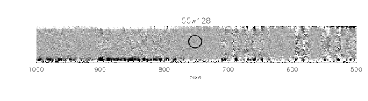
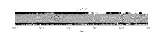
Figure 14: continued

Figure 15: continued

Figure 16: continued

Figure 17: continued

References

- (1) Barbaro G. & Poggianti B. M., 1997, A&A, 324, 490
- (2) Baum S.A., Zirbel L., O’Dea C. P., 1995, ApJ, 451, 88
- (3) Bershady M.A., Hereld M., Kron R.G., Koo D.C., Munn J.A., Majewski S.R., 1994, AJ, 108, 870
- (4) Best P. N., van Dokkum P. G., Franx M., Röttgering H. J. A., 2002, MNRAS, 330, 17
- (5) Best P. N., Kauffmann G., Heckman T. M., Ivezić Ž., 2005, MNRAS, 362, 9
- (6) Best P. N., Kaiser C. R., Heckman T. M., Kauffmann G., 2006, astro–ph/0602171
- (7) Blanton M. R. et al., 2001, AJ, 121, 2358
- (8) Bower R. G., Benson A. J., Malbon R., Helly J. C., Frenk C. S., Baugh C. M., Cole S., Lacey C. G., 2006, MNRAS, 370, 645
- (9) Bruzual G., Charlot S., 2003, MNRAS, 344, 1000
- (10) Casali M. & Hawarden T., 1992, UKIRT Newsletter, 4, 33
- (11) Clewley L. & Jarvis M., 2004, MNRAS, 352, 909
- (12) Condon J. J. & Yin Q. F., 1990, ApJ, 357, 97
- (13) Dunlop J.S. & Peacock J.A., 1990, MNRAS, 247, 19
- (14) Eales S., Rawlings S., Law–Green D., Cotter G., Lacy M., 1997, MNRAS, 291, 593
- (15) Fanaroff B.L. and Riley J.M., 1974, MNRAS, 167, 31
- (16) Gawroński M. P., Marecki A., Kunert-Bajraszewska M., Kus A. J., 2006, A&A, 447, 63
- (17) Gopal-Krishna & Wiita P.J., 2000, A&A, 363, 507
- (18) Jackson C.A. & Wall J.V., 1999, MNRAS, 304, 160
- (19) Jorgensen I., 1994, PASP, 106, 967
- (20) Kauffmann G., Heckman T. M., Tremonti C., Brinchmann J., Charlot S., White S. D. M., Ridgway S. E., Brinkmann J., Fukugita M., Hall P. B., Ivezić Ž., Richards G. T., Schneider, D. P. 2003, MNRAS, 346, 1055
- (21) Koo, D. C. & Kron, R. G., 1982, A&A, 105, 107
- (22) Kron, R. G. 1980, ApJS, 43, 305
- (23) Landolt A. U., 1992, AJ, 104, 340
- (24) Ledlow M.J. & Owen F.N., 1996, AJ, 112, 9
- (25) Leggett, S. 2005, http://www.jach.hawaii.edu/UKIRT/astronomy/ calib/phot_cal/cam_zp.html
- (26) McCarthy P. J., van Breugel W., Spinard H., Djorgovski S., 1987, ApJ, 321, L29
- (27) Monet, D. G. et al. 2003, AJ, 125, 984
- (28) Oort M. J. A. & van Langevelde H. J., 1987, A&AS, 71, 25
- (29) Oort M. J. A., Katgert P., Steeman F. W. M., Windhorst R. A., 1987, A&A, 179, 41
- (30) Oort M. J. A. & Windhorst R. A., 1985, A&A, 145, 405
- (31) Owen F.N., Laing R.A., 1989, MNRAS, 238, 357
- (32) Perley R.A., 1999, in Synthesis Imaging in Radio Astronomy II, ASP Conf Ser 180, 383
- (33) Taylor M., 2000, http://www.star.bris.ac.uk/mbt/wfc/calibrate/
- (34) Sandage A., 1972, ApJ, 173, 485
- (35) Smith J.A. et al., 2002, AJ, 123, 2121
- (36) Snellen I. A. G. & Best P. N., 2001, MNRAS., 328, 897
- (37) Snellen I. A. G., Bremer M. N., Schilizzi R. T., Miley G. K., van Ojik R., 1996, MNRAS, 279, 1294
- (38) Stoughton C. et al., 2002, AJ, 123, 485
- (39) Wall J.V., 1980, Phil. Trans. R. Soc., A296, 367
- (40) Waddington I., Windhorst R.A., Dunlop J.S., Koo D.C., Peacock J.A., 2000, MNRAS, 317, 801
- (41) Waddington I., Dunlop J.S., Peacock J.A., Windhorst R.A., 2001, MNRAS, 328, 882
- (42) Willott C. J., Rawlings, S., Blundell K. M., Lacy M., 1999, MNRAS, 309, 1017
- (43) Willott C.J., Rawlings S., Blundell K.M., Lacy M., Eales S.A., 2001, MNRAS., 322, 536
- (44) Willott C. J., Rawlings, S., Jarvis M. J., Blundell K. M., 2003, MNRAS, 339, 173
- (45) Windhorst R.A., van Heerde G.M., Katgert P., 1984, A&AS, 58, 1
- (46) Windhorst R. A., Mathis D., Neuschaefer L., 1990, in R. G. Kron (ed.), ASP Conf. Ser. 10: Evolution of the Universe of Galaxies, pp389–403
- (47) Windhorst R. A., Fomalont E. B., Partridge R. B., Lowenthal J. D., 1993, ApJ, 405, 498
- (48) York D.G. et al., 2000, AJ, 120, 1579
- (49) Zirbel E.L. & Baum S.A., 1995, ApJ, 448, 521