Study of Di-Pion Transitions
Among $\Upsilon(3S)$, $\Upsilon(2S)$, and $\Upsilon(1S)$ States

Abstract

We present measurements of decay matrix elements for hadronic transitions of the form $\Upsilon({n}S)\rightarrow\Upsilon({m}S)\pi\pi$, where $(n,m)=(3,1),(2,1),(3,2)$. We reconstruct charged and neutral pion modes with the final state Upsilon decaying to either $\mu^{+}\mu^{-}$ or $e^{+}e^{-}$. Dalitz plot distributions for the twelve decay modes are fit individually as well as jointly assuming isospin symmetry, thereby measuring the matrix elements of the decay amplitude. We observe and account for the anomaly previously noted in the di-pion invariant mass distribution for the $\Upsilon({3}S)\rightarrow\Upsilon({1}S)\pi\pi$ transition and obtain good descriptions of the dynamics of the decay using the most general decay amplitude allowed by partial conservation of the axial-vector current (PCAC) considerations. The fits further indicate that the $\Upsilon({2}S)\rightarrow\Upsilon({1}S)\pi\pi$ and $\Upsilon({3}S)\rightarrow\Upsilon({2}S)\pi\pi$ transitions also show the presence of terms in the decay amplitude that were previously ignored, although at a relatively suppressed level.

I Introduction

The transitions $\Upsilon({n}S)\rightarrow\Upsilon({m}S)\pi\pi$ are of particular interest as probes of heavy quark and low energy QCD systems. The large $b$ quark mass causes the $b\bar{b}$ bound state to have a very small radius ($\sim 1$ GeV^-1) and to be non-relativistic ($(v/c)^{2}\approx 0.1$). This makes these transitions ideal to study the process by which a pion pair is excited from the vacuum by the gluon field. The transitions among the massive bound states making up the $\Upsilon({n}S)$ family can be calculated in terms of multipole moments of the chromo-dynamic field, providing simple relative rate and transition rule predictions. The pion pair excitation can be factored out and approximated separately. Most recent theoretical work has concentrated on this latter aspect of the decays.

The $\eta^{\prime}\rightarrow\eta\pi\pi$ transition was the first decay of this form studied London66 , followed some years later by the $\psi^{\prime}\rightarrow J/\psi\pi\pi$ transition psiprime . The $\eta^{\prime}$ decay is only barely above threshold, and so the transition cannot show significant structure. Detailed study of the kinematics confirmed this. In contrast to this, the $\psi^{\prime}$ decay has decay dynamics very different from a phase space distribution. The di-pion invariant mass distribution of this decay shows strong enhancement at larger values of ${M_{\pi\pi}}$. However, this is consistent with the presence of only the simplest term in the general Lorentz invariant amplitude derived from PCAC considerations Brown and Cahn (1975); MBVoloshin:75 . This is supported by the isotropic decay angular distribution of the pions, implying a minimal $D$-wave component.

Previous CLEO data have been used to study $\Upsilon({n}S)\rightarrow\Upsilon({m}S)\pi\pi$ transitions Butler et al. (1994); Glenn et al. (1999); Alexander et al. (1998); Brock et al. (1991), with the $\Upsilon({2}S)\rightarrow\Upsilon({1}S)\pi\pi$ and $\Upsilon({3}S)\rightarrow\Upsilon({2}S)\pi\pi$ transitions following this same pattern in the di-pion invariant mass spectra as for the lighter mesons. But the $\Upsilon({3}S)\rightarrow\Upsilon({1}S)\pi\pi$ transition has a second, strong rate enhancement near the $\pi\pi$ invariant mass threshold. This enhancement and the accompanying depletion at intermediate invariant mass are inconsistent with either pure phase space or the simple matrix element describing the $\psi^{\prime}\rightarrow J/\psi\pi\pi$ observations. Either another term must be included in the Lorentz invariant matrix element, or one must question the applicability of PCAC to the pion excitation and the validity of the multipole expansion of the $b\bar{b}$ bound state.

Various mechanisms have been suggested to explain this anomaly, such as (i) large contributions from final state interactions BDM ; CKK , (ii) a $\sigma$ isoscalar resonance in the $\pi\pi$ system KII ; Uehara , (iii) exotic $\Upsilon-\pi$ resonances VoloshinJTEP ; BDM ; ABSZ ; GSCP , (iv) an ad hoc constant term in the amplitude Moxhay , (v) coupled channel effects LipkinThuan ; ZK , (vi) $S-D$ mixing CKK2 , and (vii) relativistic corrections Voloshin (2006).

More recent experimental analyses with the very large data sets accumulated by the $B$ factories at the $\Upsilon({4}S)$ show interesting behavior as well. Belle Abe et al. (2005) and $B$a$B$ar BaBar4S2S1S do not see such anomalous behavior in the $\Upsilon({4}S)\rightarrow\Upsilon({1}S)\pi\pi$ transition, but $B$a$B$ar does see such a double peaked structure in the $\Upsilon({4}S)\rightarrow\Upsilon({2}S)\pi\pi$ transition.

The shapes of the decay distributions originate in the details of the excitation of the pion pair from the vacuum and the particular projection of the initial state onto the final state. Hence, the enhancement of the decay rate at low ${M_{\pi\pi}}$, thus far considered an anomaly, is a good probe of the details of low energy QCD in the transitions of the bound states and the excitation of light hadrons from the vacuum.

The general matrix element constrained by PCAC was derived by Brown and Cahn Brown and Cahn (1975) and is further constrained by treating the Upsilon transition as a multipole expansion as derived by Gottfried Gottfried (1978), Yan Yan (1980), Voloshin and Zakharov Voloshin and Zakharov (1980), and others. The general transition amplitude is then given in non-relativistic form:

$${\cal M}={\cal A}{({\epsilon^{\prime}}\cdot{\epsilon})}(q^{2}-2M_{\pi}^{2})\,+{\cal B}{({\epsilon^{\prime}}\cdot{\epsilon})}E_{1}E_{2}+{\cal C}((\epsilon^{\prime}\cdot q_{1})(\epsilon\cdot q_{2})+(\epsilon^{\prime}\cdot q_{2})(\epsilon\cdot q_{1}))~{},$$ (1)

where ${\epsilon^{\prime}}$ and ${\epsilon}$ are the polarization vectors of the parent and final state Upsilons, and $q_{1,2}$ are the four-momenta of the pions. In the first term, $q^{2}$ is the invariant mass of the pion pair. The quantities $E_{1}$ and $E_{2}$ are the energies of the two pions in the parent rest frame, essentially indistinguishable from the lab frame due to the large masses of the Upsilons. The third, or “${\cal C}$” term in this expression couples transitions via the chromo-magnetic moment of the bound state $b$ quarks, hence requiring a spin flip. This is expected to be highly suppressed by the large mass of the $b$ quark, so we expect only the first two terms to contribute. Neglecting the dependence on the parent and final state Upsilon polarizations (which apply only to the ${\cal C}$-term), we have only two degrees of freedom, the Dalitz variables $q^{2}=M^{2}_{\pi\pi}$ and $r^{2}=M^{2}_{\Upsilon\pi}$. In writing this amplitude, we have assumed the chiral limit, so that a fourth term, $gM_{\pi}^{2}$, is taken to be zero MannelUrech ; newVoloshin .

The expression in Eqn. 1 can be made fully Lorentz invariant by rewriting the energy product in the ${\cal B}$ term as

$$E_{1}E_{2}\approx[(P^{\prime}\cdot q_{1})(P\cdot q_{2})+(P^{\prime}\cdot q_{2})(P\cdot q_{1})]/[2M_{\Upsilon^{\prime}}M_{\Upsilon}],$$ (2)

with ${P^{\prime}}$ and ${P}$ being the initial state and final state $\Upsilon$ four-momenta.

The quantities ${\cal A}$, ${\cal B}$, and ${\cal C}$ are form factors that depend on the detailed dynamics of the decay. They are in principle functions of the Dalitz variables $q^{2}$ and $r^{2}$. However, we expect them to vary on the scale of $\Lambda_{\rm QCD}$, which is comparable to the total energy release of the decays, so to first order we assume they are complex constants. Angular structure or ${M_{\pi\pi}}$ dependence beyond that indicated in the explicit amplitude, Eqn. 1, would be an indication of the non-constancy of these form factors, or alternately the breakdown of the assumptions leading to Eqn. 1.

The di-pion transition can be interpreted as taking place in sequential two-body decays through a fictitious intermediate state $X$ via the chain $\Upsilon({n}S)\rightarrow\Upsilon({m}S)X$ and $X\rightarrow\pi\pi$ (see Fig. 1). In this view we can define the helicity angle of the $X\rightarrow\pi\pi$ decay in the usual manner of the Jacob and Wick formalism. The polar helicity angle is referred to as $\theta_{X}$. Its cosine is used interchangeably with the second Dalitz variable, $r^{2}$, as they are linearly related:

$$2r^{2}=2M_{\pi}^{2}+M_{\Upsilon^{\prime}}^{2}+M_{\Upsilon}^{2}-q^{2}-\cos\theta_{X}\sqrt{\frac{1}{q^{2}}\left(q^{2}-4M_{\pi}^{2}\right)\Lambda_{3}(M_{\Upsilon^{\prime}}^{2},M_{\Upsilon}^{2},q^{2})}$$ (3)

where $\Lambda_{3}(a,b,c)=a^{2}+b^{2}+c^{2}-2ab-2ac-2bc$. These variables ($r^{2}$ or $\cos\theta_{X}$) carry structure from the second term in the amplitude due to the following relation:

$$E_{1}E_{2}=\frac{1}{4}\left((E_{1}+E_{2})^{2}-\Delta E^{2}_{\rm max}\cos^{2}\theta_{X}\right)~{},$$ (4)

with $\Delta E\equiv E_{2}-E_{1}$. Because the initial state and final state Upsilons are essentially at rest, the energy sum $E_{1}+E_{2}$ is nearly a constant and equal to the mass difference between the Upsilons. For the $\pi^{+}\pi^{-}$ final state, $\theta_{X}$ is defined as the angle of the positive pion, with $-1<\cos\theta_{X}<1$; for the $\pi^{0}\pi^{0}$ final state, because one cannot distinguish between the two neutral pions, we take $0<\cos\theta_{X}<1$.

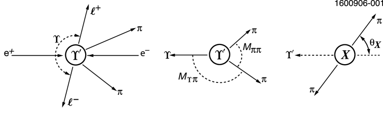
Figure 1: (Left) The decay $\Upsilon({n}S)\rightarrow\Upsilon({m}S)\pi\pi$ follows the production of an initial state labeled $\Upsilon^{\prime}$ which decays to an $\Upsilon\pi\pi$ state. In our analysis, the final state $\Upsilon$ decays to a lepton pair whose momentum vectors are very nearly back-to-back due to the large energy release. (Center) The decay of the initial state Upsilon is governed by two kinematic variables, the Dalitz masses $M_{\Upsilon\pi}$ and $M_{\pi\pi}$. (Right) Alternately one can think of the $\pi\pi$ system as a composite, $X$, and study its structure via the pion “decay” angles.

Finding the presence of a non-zero ${\cal C}$ term would indicate the breakdown of the multipole expansion, i.e., of the assumption that the pion pair excitation is independent of the Upsilon transition process from $n^{3}S_{1}$ state to $m^{3}S_{1}$, and that the spin flip of the $b$ quarks is suppressed. However, finding a non-zero ${\cal C}$ term could also be due to distortions of the distribution not accountable for by using only the first two terms with complex, but constant, coefficients ${\cal A}$ and ${\cal B}$.

II Data Sets and Event Selection

Data were collected with the CLEO III detector which is described in detail elsewhere Viehhauser (2001); Peterson et al. (2002); Artuso et al. (2005). In this analysis we observe $e^{\pm}$, $\mu^{\pm}$, $\pi^{\pm}$, and $\gamma$ particles in the final state, and so use both the tracking and calorimetry information from the detector, as well as lepton identification. Thus we employ global event, track, lepton, shower, and neutral pion selection criteria, in addition to signal and background identification criteria.

The data were taken while running on the $\Upsilon({3}S)$ resonance, subject to standard CLEO data quality selections, and represent an integrated luminosity of $1.14\,{\rm{\rm fb}^{-1}}$, and an $\Upsilon({3}S)$ production yield of $(4.98\pm 0.01)\times 10^{6}$. The $\Upsilon({2}S)$ sample is obtained by reconstruction of sequential decays, $\Upsilon({3}S)\rightarrow\Upsilon({2}S)\,+\,{\rm anything}$, occurring in this sample. The $\Upsilon({2}S)$ population of $(5.27\pm 0.40)\times 10^{5}$ is estimated from the branching fraction Yao et al. (2006) of $10.6\%\pm 0.8\%$ for the decay $\Upsilon({3}S)\rightarrow\Upsilon({2}S)\,+\,{\rm anything}$, which is dominated by pion pair transitions and sequential photon decays through the $\chi_{b}$(2P) states.

All integrals needed in the analysis (for evaluation of acceptances and efficiencies) are calculated via the Monte Carlo method. Physics event generation is performed using the Lund Monte Carlo Sjostrand:2001yu embedded in the CLEO physics Monte Carlo QQ QQ . The Lund event generator is used because it accurately accounts for the physics of the QCD bound state production. The $\Upsilon({3}S)$ produced in the $e^{+}e^{-}$ collision is then decayed according to standard decay tables and the detector response to the decay products is simulated using the physics simulation package GEANT CER (1993).

In general, since all integrals are performed with respect to the natural measure over phase space, only phase space decays need be simulated. The decay amplitude is known exactly as a function of the decay kinematics, so all inputs to the matrix element extraction (other than acceptance and efficiency) are known to the precision of detector reconstruction.

We select events containing two leptons ($\mu^{+}\mu^{-}$ or $e^{+}e^{-}$) and two pions ($\pi^{+}\pi^{-}$ or $\pi^{0}\pi^{0}$). All low momentum tracks are assumed to be pions, because there is insufficient phase space for the production of a pair of kaons in a transition among any two of the three bound state Upsilons. Electrons and muons are identified by their energy loss and penetration depth in the detector as detailed below, and are required to be consistent with originating from either an $\Upsilon({2}S)$ or an $\Upsilon({1}S)$ decay. The pion candidates are constrained to come from a common point at the beam location and the recoil mass ($M_{\rm rec}^{2}=P_{\rm rec}\cdot P_{\rm rec};P_{\rm rec}\equiv P_{\rm beam}-q_{1}-q_{2}$; see below) is used to identify the transition. The lepton pair invariant mass spectra and the recoil mass spectra are shown in Figs. 2 and 3, respectively.

Figure 2: Di-lepton invariant mass distributions for lepton pairs; the abscissa is the di-lepton invariant mass, showing peaks at the masses of the $\Upsilon({1}S)$ and $\Upsilon({2}S)$ mesons. The hatching indicates the limits to the invariant mass selection windows. Candidates are plotted after the signal selection described in Section II.D. At left are the di-muon candidates and at right the di-electron candidates.

Figure 3: Recoil mass, $M_{\rm rec}$, distributions for all modes. The upper plot is generated from neutral decays, $\Upsilon({n}S)\rightarrow\Upsilon({m}S)\pi^{0}\pi^{0}$ and the lower from charged decays, $\Upsilon({n}S)\rightarrow\Upsilon({m}S)\pi^{+}\pi^{-}$. The final signal selections (track quality, pion quality, di-lepton mass, etc.) have been applied. The peaks at the $\Upsilon$(1S) and $\Upsilon$(2S) masses correspond to decays to these resonances from an $\Upsilon$(3S) parent. The peaks at 9.8 GeV/$c^{2}$ are from $\Upsilon$(2S)$\to\Upsilon$(1S)$\pi\pi$ decays. The hatching shows the bounds on the recoil mass values for the three transitions. See also the window definitions in Tab. 1. Yields are set to zero in the regions that correspond neither to signal nor to sidebands.

II.1 Global Event Selection

The data used in this analysis are required to have been taken while running on the $\Upsilon({3}S)$ resonance energy. Global event characteristics are used to preselect the events. Excessive tracks or showers in an event can dramatically increase the combinatoric background. To avoid this, reconstructed events are selected subject to upper limits on number of charged particle tracks and number of calorimeter showers. To establish conservative limits, signal Monte Carlo is studied for $\Upsilon({2}S)\rightarrow\Upsilon({1}S)\pi\pi$ transitions, which are the “worst case”, in that extra tracks and showers in these modes arise from the initial transition from the $\Upsilon({3}S)$ to the $\Upsilon({2}S)$. Neglecting stray particles and secondary showers, there should be no more than four low momentum charged particle tracks and no more than eight electromagnetic showers in signal events. Comparison between data and Monte Carlo show good agreement in the number of tracks and showers found in the selected events.

II.2 Selection of Final State Particles

All candidate charged tracks are required to satisfy quality criteria. They must:

• come from within $5\,{\rm{\rm cm}}$ of the origin along the beam axis (detector $\hat{z}$ axis);

• come within $5\,{\rm{\rm mm}}$ of the beam axis (impact parameter);

• have momentum less than the beam energy;

• have a good helix track fit, with $\chi^{2}$ per hit less than 20.

These requirements are applied to all track candidates and are augmented with identification criteria for leptons (see below) before being accepted as decay candidates.

The charged transition pions frequently are of such low transverse momentum that they make two or more semi-circular arcs in the tracking volume. These “excess” tracks are removed by comparing the helix parameters, taking into account the expected energy loss as these pions spiral through the drift chamber.

Candidate muons and electrons are required to have high momentum by requiring their transverse momentum to be $p_{T}>1$ GeV/$c$, which removes a large fraction of the events with non-leptonic Upsilon decays. Because the leptons we seek originate from the decay of objects more massive than $9.4\,{\rm{\rm GeV}/c^{2}}$, they pass this requirement easily.

Muons are selected from among good tracks and are additionally required to penetrate the muon chambers to a depth of at least three interaction lengths. The ratio of energy deposition in the calorimeter to track momentum must also be less than one half, $E/pc<0.5$.

Electrons are selected from among good tracks and are additionally required to have a ratio of energy deposited in the calorimeter to track momentum $E/pc>0.5$, as well as having a profile of energy deposition consistent with that of an electromagnetic shower and a good spatial match between the shower and the track. The $E/pc$ ratio selection is a very loose requirement added only as a precaution against muons contaminating the electron sample.

The di-lepton mass is loosely required to be that of the final state Upsilon being studied, as shown in Fig. 2. For the $\Upsilon$(1S) we require $9.25<M_{\ell\ell}<9.75$ GeV/$c^{2}$, while for the $\Upsilon$(2S) we demand $M_{\ell\ell}>9.85$ GeV/$c^{2}$. Due to the large widths of these invariant mass peaks, no side band selection is performed in this variable, but rather only in the recoil mass distribution.

The $\pi^{0}$ candidates are reconstructed from photon pairs. This begins by applying selection criteria to the showers. To be considered a photon, a shower must:

• have energy greater than $30\,{\rm{\rm MeV}}$;

• have a lateral shower profile consistent with that of a photon;

• be inconsistent with the extrapolation of any track in the detector;

• not include noisy channels in the calorimeter;

• not be in the overlap region between the barrel and endcap calorimeter modules;

• not be in the ring of crystals closest to the beam axis.

Showers satisfying these selection criteria are considered to be photons and are combined into $\pi^{0}$ candidates. Photon pairs are required to have an invariant mass within $50\,{\rm{\rm MeV}/c^{2}}$ of the nominal $\pi^{0}$ mass, $M_{\pi^{0}}$. They are then required to fall within the asymmetric window

$$-4<\frac{M_{\gamma\gamma}-M_{\pi^{0}}}{\sigma_{\gamma\gamma}}<3~{}.$$ (5)

The photon-pair mass resolution, $\sigma_{\gamma\gamma}$, is typically 5-7 MeV/$c^{2}$. Candidate photon pairs are then kinematically constrained (subject to the measured uncertainties on energies and shower spatial locations) to have an invariant mass equal to $M_{\pi^{0}}$. To be used, $\pi^{0}$ candidates are further required to have a successful kinematic fit with confidence level (one degree of freedom) greater than $0.1\%$.

II.3 Recoil Mass and Signal and Background Regions

We select events for each transition by cutting on the mass of the system recoiling against the two pions in the $\Upsilon^{\prime}\rightarrow\pi\pi+$”anything” decay: $M^{2}_{\rm rec}=M^{2}_{\Upsilon^{\prime}}+q^{2}-2q\cdot P^{\prime}$, where, as above, $q=q_{1}+q_{2}$ and $P^{\prime}$ is the Lorentz momentum of the initial state Upsilon. Given the large mass of the initial state Upsilon, the dot product simplifies and the recoil mass can be well approximated by $M^{2}_{\rm rec}\approx M^{2}_{\Upsilon^{\prime}}+q^{2}-2M_{\Upsilon^{\prime}}(E_{1}+E_{2})$. For the cascade decays, $\Upsilon({2}S)\rightarrow\Upsilon({1}S)\pi\pi$, this is not quite correct because the Lorentz momentum of the initial state Upsilon (the $\Upsilon({2}S)$) is not equal to the beam momentum. However, because the total momentum of the pions is small and the initial state is approximately at rest, using the incorrect momentum for the initial state does not significantly change the recoil mass distribution other than to shift it by the difference between $\Upsilon({3}S)$ and $\Upsilon({2}S)$ masses. Hence, we expect to find three recoil mass peaks. The transitions originating from the $\Upsilon({3}S)$ will generate recoil mass ($M_{\rm rec}$) peaks at the masses of the $\Upsilon({1}S)$ and $\Upsilon({2}S)$, while the $\Upsilon({2}S)\rightarrow\Upsilon({1}S)\pi\pi$ decays will yield a peak at $9.79\,{\rm{\rm GeV}/c^{2}}$. These three peaks are clearly visible in Fig. 3.

The recoil mass, $M_{\rm rec}$, is measured rather accurately, especially in the charged case, due to the good resolution on the momenta of the low-momentum pions. It is still quite good for the neutral modes where the total pion momentum is given as the sum of momenta of two $\pi^{0}$ candidates reconstructed from the calorimeter showers.

II.4 Signal and Background Selection

The fit requires signal and background samples. They are determined as a function of the recoil mass, $M_{\rm rec}$, only. The recoil mass peak widths are determined from Monte Carlo with tight selections on variables other than the recoil mass. These widths are then used to determine mass windows to select events in both Monte Carlo and data samples. The signal regions are defined as the range within three times the peak width of the nominal recoil mass, while the backgrounds are the regions from six to twelve times the peak width from the nominal mass above and below the peak mass. The masses and widths used to define these regions are listed in Table 1. The width of the recoil mass distribution in the decays $\Upsilon({2}S)\rightarrow\Upsilon({1}S)\pi^{+}\pi^{-}$ is roughly twice that of the direct decays. This is due to the boost of the initial state Upsilon imparted in its production by the cascade from the $\Upsilon({3}S)$. The edges of the signal windows are indicated by the hatching in Fig. 3. Note that in Fig. 3 the yield in the regions not used for either signal or background definition have been set to zero.

The Dalitz plot distributions for the selected data in six of the twelve final states are shown in Figs. 4 and  5. Comparison of the $\pi^{0}\pi^{0}$ and $\pi^{+}\pi^{-}$ for the $\Upsilon({3}S)\rightarrow\Upsilon({1}S)\pi\pi$ shows the depletion in charged particle efficiency at moderate di-pion invariant mass and large $|{\rm cos}~{}\theta_{X}|$. Comparison of the charged modes for $\Upsilon({3}S)\rightarrow\Upsilon({1}S)\pi^{+}\pi^{-}$ and $\Upsilon({2}S)\rightarrow\Upsilon({1}S)\pi^{+}\pi^{-}$ shows, in two dimensions, the obvious disparity between the two distributions.

Figure 4: Candidate events that passed all selection criteria, and that have the final state Upsilon decaying to $\mu^{+}\mu^{-}$. In the middle is the decay $\Upsilon({3}S)\rightarrow\Upsilon({1}S)\pi^{+}\pi^{-}$. To the left is its neutral counterpart $\Upsilon({3}S)\rightarrow\Upsilon({1}S)\pi^{0}\pi^{0}$. To the right is the charged transition $\Upsilon({2}S)\rightarrow\Upsilon({1}S)\pi^{+}\pi^{-}$, with the bulk of its distribution at large values of dipion invariant mass. In each plot there are ten degrees of grey-scale ranging from white (lowest occupancy per bin) to black (highest occupancy).

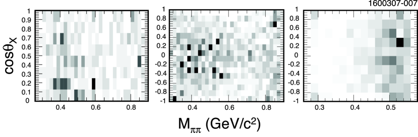
Figure 5: Candidate events that have passed all selection criteria, and that have the final state Upsilon decaying to $e^{+}e^{-}$. As in the prior plot, three transitions are, left to right, $\Upsilon({3}S)\rightarrow\Upsilon({1}S)\pi^{0}\pi^{0}$, $\Upsilon({3}S)\rightarrow\Upsilon({1}S)\pi^{+}\pi^{-}$, and $\Upsilon({2}S)\rightarrow\Upsilon({1}S)\pi^{+}\pi^{-}$.

Transition Recoil Mass Width (Data) Width (MC) Width (Cut) (${\rm MeV}/c^{2}$) (${\rm MeV}/c^{2}$) (${\rm MeV}/c^{2}$) (${\rm MeV}/c^{2}$) $\Upsilon({3}S)\rightarrow\Upsilon({1}S)\pi^{+}\pi^{-}$ 9 460.4 2.4 2.5 2.5 $\Upsilon({2}S)\rightarrow\Upsilon({1}S)\pi^{+}\pi^{-}$ 9 792.4 5.0 5.0 5.0 $\Upsilon({3}S)\rightarrow\Upsilon({2}S)\pi^{+}\pi^{-}$ 10 023.3 2.2 1.9 2.1 $\Upsilon({3}S)\rightarrow\Upsilon({1}S)\pi^{0}\pi^{0}$ 9 460.4 15.0 12.7 13.8 $\Upsilon({2}S)\rightarrow\Upsilon({1}S)\pi^{0}\pi^{0}$ 9 792.4 10.9 10.5 10.7 $\Upsilon({3}S)\rightarrow\Upsilon({2}S)\pi^{0}\pi^{0}$ 10 023.3 3.4 3.4 3.4

Table 1: Recoil mass distribution central values and widths for the signal and background selections used in the fit. The central values and the widths agree well between data and Monte Carlo. The signal windows are defined as the region within three times the cut width (last column) of the central mass and the background windows are defined as the region from six to twelve cut widths from the center on either side. The background subtraction is only important for the cascade decays for which there is a large contribution to the signal region from event combinatorics.

III Matrix Element Fits

III.1 The Likelihood Fitter

The binned likelihood fit to the kinematic distributions of the $\Upsilon$(mS)$\rightarrow\Upsilon$(ns)$\pi\pi$ decays is designed to deal correctly with the low bin yields expected from dividing approximately 2000 events over a two dimensional space with more than ten bins per dimension. The general case of this problem is solved in Ref. Barlow and Beeston (1993). Specific details of our application of this technique, including notes on variable smearing and background inclusion, are found in the Appendix. We fit the decay distributions to a product of the squared modulus of the decay amplitude and the phase space density sculpted by the detector acceptance. The matrix element has a known analytical form (see Eqn. 1) as a function of the form factors ${\cal A}$, ${\cal B}$, and ${\cal C}$, which are taken as complex constants. Its leading angular structure is known, and so long as the form factors are known, too, the entire amplitude can be described exactly. However, we cannot model the detector acceptance in analytic form, so we approximate its effect via Monte Carlo integration.

We determine the integral of the phase space density in a bin in ($q^{2},{\rm cos}~{}\theta_{X}$), sculpted by acceptance and efficiency, by counting Monte Carlo events that pass the selection criteria and fall into that bin. In Fig. 6 we show the two-dimensional phase space after such sculpting. Note that while the overall efficiency for the neutral final state is lower than for its charged counterpart, the former is more uniform, particularly in the regions of intermediate $M_{\pi\pi}$ and large $|{\rm cos}~{}\theta_{X}|$. For each bin of the observed distribution we predict the number of events as a function of the matrix element parameters by multiplying the Monte Carlo integral for that bin by the exactly calculated matrix element value for that bin. This approach avoids generating Monte Carlo integrated templates for each component of the angular distribution and reduces the uncertainty due to finite Monte Carlo sample size.

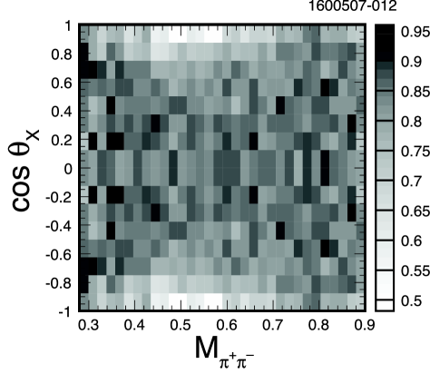
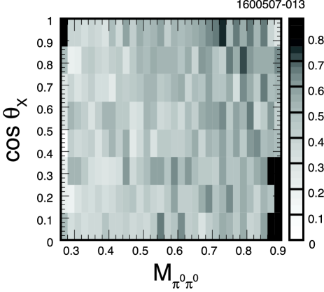
Figure 6: The efficiency-sculpted phase space in the two-dimensional plane for the transitions $\Upsilon$(3S)$\to\Upsilon$(1S)$\pi^{+}\pi^{-}$ (left) and $\Upsilon$(3S)$\to\Upsilon$(1S)$\pi^{0}\pi^{0}$ (right). Note that the neutral final state has a more uniform efficiency, especially in the region of moderate di-pion mass and large $|{\rm cos}(\theta_{X})|$.

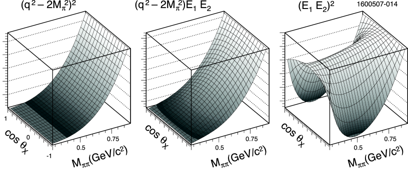
Figure 7: The three functions used in the fit for the $\Upsilon$(3S) decay to $\Upsilon$(1S)$\pi\pi$. From left to right these are for the pure ${\cal A}$ term, the interference term, and the pure ${\cal B}$ term.

To fit the decay distribution we take the squared modulus of the decay amplitude, Eqn. 1, and decompose it as a sum of six functional forms each multiplied by one of $|{\cal A}|^{2}$, $|{\cal B}|^{2}$, $|{\cal C}|^{2}$, $\Re({\cal A}^{*}{\cal B})$, $\Re({\cal A}^{*}{\cal C})$, or $\Re({\cal B}^{*}{\cal C})$. For normalization, the matrix element ${\cal A}$ is set to unity.

The functional forms (e.g., $(q^{2}-2M_{\pi}^{2})^{2}$) depend on the Dalitz variables and are pre-evaluated into templates over the Dalitz space. The fitter then seeks the best fit as a function of the matrix element ratios ${\cal A}$, ${\cal B}$, and ${\cal C}$. The input to the fitter consists of only the data, background, and phase space Monte Carlo binned across the Dalitz plot, and the component templates of the decay distribution derived from the exact decay amplitude, but taking into account the kinematic smearing and acceptance and efficiency effects due to reconstruction as determined from the detector simulation. The backgorund component is scaled by the ratio of the signal region width (6 $\sigma$; see Section II.D) to the total backgorund sideband width (nominally 12$\sigma$).

In Fig. 7 we show the functional forms for $|{\cal A}|^{2}$, $\Re({\cal A}^{*}{\cal B})$, and $|{\cal B}|^{2}$ for the case of $\Upsilon$(3S)$\to\Upsilon$(1S)$\pi\pi$. In our experiment, the complementarity of the neutral and charged final states is particularly important in that the rightmost of these (the form for $|{\cal B}|^{2})$) depletes the region for which the $\pi^{+}\pi^{-}$ channel has falling efficiency. Consistent results between the $\pi^{0}\pi^{0}$ and $\pi^{+}\pi^{-}$ transitions gives us confidence that the simulation of this fall-off in efficiency is reliable. The matrix element extraction procedure is tested “end-to-end” by simulating signal with known matrix elements in Monte Carlo and comparing the fit result and its uncertainty with the known inputs. Samples of the same size as the observed yield are generated and fit identically to the data. The results yield standard normal distributions in the observed uncertainty scaled residuals for widely distributed seed matrix element values. This confirms the fitter is unbiased at the level of precision to be expected from the sample size of the measurement.

III.2 Fits with ${\cal C}=0$

The fits to the two dimensional distributions of ${M_{\pi\pi}}$ and $\cos\theta_{X}$ determine the matrix element ${\cal B}/{\cal A}$ and ${\cal C}/{\cal A}$. The extracted values of $\Re({\cal B}/{\cal A})$ and $\Im({\cal B}/{\cal A})$ are summarized in Table 2, subject to the constraint that ${\cal C}\equiv 0$. In that we only measure the cosine of the phase difference between ${\cal B}$ and ${\cal A}$, $\Im({\cal B}/{\cal A})$ is only known to within a sign. The upper set of matrix elements are obtained from independent fits to ten individual decay modes; we cannot individually fit the two modes associated with $\Upsilon$(3S)$\to\Upsilon$(2S)$\pi^{+}\pi^{-}$ because of their limited statistics. The lower set of three are from the simultaneous fits of all final states for each given Upsilon transition.

In the simultaneous fits the relative branching ratios between modes are not constrained, but it is assumed that the di-pion excitation dynamics is independent of the charge of the pion final state (isospin symmetry) and thus the decay distributions should be identical to within statistical fluctuations for all transitions between the same Upsilon states. This assumption is supported by the consistency among the matrix element values extracted independently, as well as their consistency with the value extracted from the simultaneous fit. In particular, the four final states studied for the transition from $\Upsilon$(3S) to $\Upsilon$(1S) show excellent agreement between the two lepton species and between charged and neutral pions.

Individual Fits $\Re({\cal B}/{\cal A})$ $\Im({\cal B}/{\cal A})$ $\Upsilon({3}S)\rightarrow\Upsilon({1}S)\pi^{+}\pi^{-}$; $\Upsilon\rightarrow\mu^{+}\mu^{-}$ $-2.514\pm 0.037$ $\pm 1.164\pm 0.059$ $\Upsilon\rightarrow e^{+}e^{-}$ $-2.527\pm 0.049$ $\pm 1.180\pm 0.079$ $\Upsilon({3}S)\rightarrow\Upsilon({1}S)\pi^{0}\pi^{0}$; $\Upsilon\rightarrow\mu^{+}\mu^{-}$ $-2.426\pm 0.085$ $\pm 1.313\pm 0.159$ $\Upsilon\rightarrow e^{+}e^{-}$ $-2.524\pm 0.093$ $\pm 1.070\pm 0.153$ $\Upsilon({2}S)\rightarrow\Upsilon({1}S)\pi^{+}\pi^{-}$; $\Upsilon\rightarrow\mu^{+}\mu^{-}$ $-0.656\pm 0.126$ $\pm 0.431\pm 0.089$ $\Upsilon\rightarrow e^{+}e^{-}$ $-0.689\pm 0.147$ $\pm 0.425\pm 0.102$ $\Upsilon({2}S)\rightarrow\Upsilon({1}S)\pi^{0}\pi^{0}$; $\Upsilon\rightarrow\mu^{+}\mu^{-}$ $-0.148\pm 0.280$ $~{}~{}0.000\pm 1.655$ $\Upsilon\rightarrow e^{+}e^{-}$ $-0.293\pm 0.330$ $\pm 0.001\pm 1.130$ $\Upsilon({3}S)\rightarrow\Upsilon({2}S)\pi^{0}\pi^{0}$; $\Upsilon\rightarrow\mu^{+}\mu^{-}$ $-0.283\pm 0.305$ $\pm 0.001\pm 1.708$ $\Upsilon\rightarrow e^{+}e^{-}$ $-0.583\pm 0.082$ $\pm 0.003\pm 1.475$ Simultaneous Fits $\Re({\cal B}/{\cal A})$ $\Im({\cal B}/{\cal A})$ $\Upsilon({3}S)\rightarrow\Upsilon({1}S)\pi\pi$ $-2.523\pm 0.031$ $\pm 1.189\pm 0.051$ $\Upsilon({2}S)\rightarrow\Upsilon({1}S)\pi\pi$ $-0.753\pm 0.064$ $\pm 0.000\pm 0.108$ $\Upsilon({3}S)\rightarrow\Upsilon({2}S)\pi\pi$ $-0.395\pm 0.295$ $\pm 0.001\pm 1.053$

Table 2: Fit results from $\Upsilon({n}S)\rightarrow\Upsilon({m}S)\pi\pi$ transitions for ${\cal B}/{\cal A}$ with ${\cal C}$ set to zero. The upper set of results is from individual fits to each separate decay mode and the lower set of results is from simultaneous fits to both lepton final states and both pion charge modes. We cannot fit the $\Upsilon({3}S)\rightarrow\Upsilon({2}S)\pi^{+}\pi^{-}$ transitions, individually in $e^{+}e^{-}$ and $\mu^{+}\mu^{-}$ or combined, because of their limited statistics. In the simultaneous fits the relative branching fractions are allowed to float. Note that we know the value of the imaginary part of the ratio only to within a sign.

To study the fit quality we project the data and the expected decay distribution for the matrix element value preferred by the fit onto the di-pion mass (${M_{\pi\pi}}$) and di-pion helicity angle ($\cos\theta_{X}$) variables and calculate a $\chi^{2}$ for each projection. To increase the bin contents we sum over lepton species but not over pion charges. We expect the shapes for charged and neutral pions to differ due to the rather different efficiencies for reconstruction and resolutions, as well as the folding of the neutral angle in the fits. Figure 8 presents plots of the data overlaid with the fit results, showing good qualitative agreement. The $\chi^{2}$ values from these overlays, given in Table 3, are acceptable, given the simplicity of the fitted matrix element.

Upsilon $\pi^{+}\pi^{-}$ $\pi^{0}\pi^{0}$ Transition $\cos\theta_{X}$ $M_{\pi\pi}$ $\cos\theta_{X}$ $M_{\pi\pi}$ $3S\to 1S$ 33.2 (16) 46.9 (32) 4.3 (8) 52.1 (32) $2S\to 1S$ 6.1 (10) 22.7 (12) 3.4 (5) 13.7 (12) $3S\to 2S$ 7.1 (7) 7.8 (6) 7.4 (4) 2.5 (7)

Table 3: The figure of merit for each of the twelve projections in the accompanying figure. For each projection we give the value of $\chi^{2}$ and, in parentheses, the number of bins used to calculate it. Uncertainties in the fit results due to limited simulation statistics are not included in these calculations.

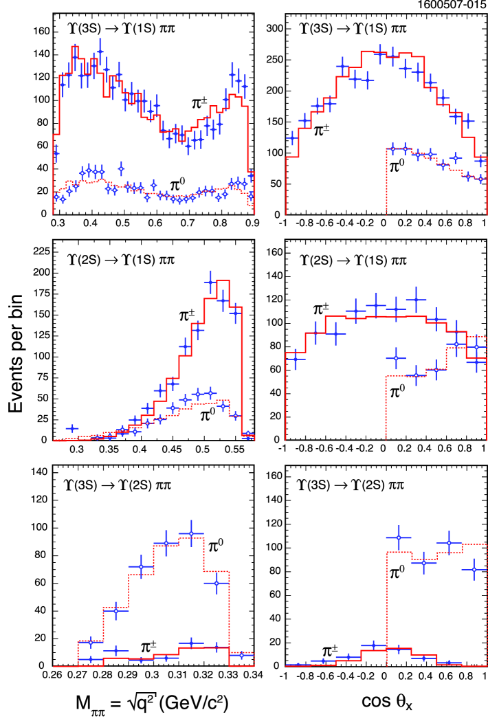
Figure 8: Plots overlaying projections of the data (points with error bars) and the fit result (histograms) onto the ${M_{\pi\pi}}$ and $\cos\theta_{X}$ variables. The plots are summed over electrons and muons, but are differentiated by pion charge. The neutral modes (open symbols, dashed lines) show only a positive distribution in $\cos\theta_{X}$ because the two pions are indistinguishable. For the charged modes (solid symbols, solid lines) the angle is that of the $\pi^{+}$.

As a further fit quality test, we examine the two dimensional distribution over the Dalitz variables of error-normalized deviations. The deviations, $\delta_{i}$, are the difference, fit subtracted from the data, divided by the mutual uncertainty:

$$\delta_{i}=\frac{d_{i}-\tilde{d}_{i}}{\sigma_{i}},$$ (6)

where each $\tilde{d}_{i}$ is the predicted decay population in bin $i$. The bin-by-bin uncertainties, $\sigma_{i}$, are composed of the uncertainty on the data yield in the bin, $\sigma_{d}=\sqrt{d_{i}}$, and the uncertainty on the template function, dominated by the fluctuation in the Monte Carlo phase space yield and proportional to $1/\sqrt{a_{i}}$, where $a_{i}$ is the Monte Carlo phase space yield in bin $i$. Hence, $\sigma_{i}=\sqrt{d_{i}+\tilde{d}_{i}^{2}/a_{i}}$.

The bins for which $d_{i}=0$ require special treatment, and $\sigma_{i}$ is modified appropriately. To minimize the effect of such bins with zero yield, we sum over muon and electron final states. This takes a weighted average over the distributions, rather than taking account of the differences between the individual distributions and their individual template predictions.

The deviations between the data and the fit templates, $\delta_{i}$, are shown in Fig. 9 for the charged and neutral transitions between $\Upsilon$(3S) and $\Upsilon$(1S). No significant bunching is observed that would indicate a bias. We neglect the small accumulations in the areas of low tracking efficiency (at large $|\cos\theta_{X}|$ and intermediate ${M_{\pi\pi}}$), probably attributable to the Monte Carlo detector model not being sufficiently accurate.

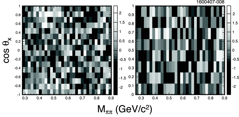
Figure 9: Plots of the bin by bin deviations of the data from the fit templates normalized to the expected uncertainty on the bin content for the transitions between $\Upsilon$(3S) and $\Upsilon$(1S). The left plot is for the charged pion modes while the right plot is for the neutral pion modes. The data are summed over lepton species. No strong concentration of deviations is apparent.

III.3 Fits Including the Chromo-magnetic Term ${\cal C}$

The fit results in Table 2 do not take into account the possible presence of amplitude terms that come from chromo-magnetic couplings, which would allow the additional ${\cal C}$ term to appear. This term is nearly degenerate with the ${\cal B}$ term, and fits allowing it to float show a strong covariance between these two terms. This is caused by the similarity in structure of the two terms; ${\cal B}$ accompanies a functional dependence $E_{1}E_{2}$, while $(\epsilon^{\prime}\cdot q_{1,2})(\epsilon\cdot q_{2,1})$ emphasizes the regions of phase space in which the pion spatial momentum, and hence also the energy, are large. The low yield modes do not allow the measurement of the term at all. We therefore only study it in the $\Upsilon({3}S)\rightarrow\Upsilon({1}S)\pi\pi$ transitions, and then only extract a value from the simultaneous fit.

The covariance between ${\cal B}$ and ${\cal C}$ for the $\Upsilon({3}S)\rightarrow\Upsilon({1}S)\pi\pi$ transition is summarized in Fig. 10, which shows the variation of extracted $|{\cal B}/{\cal A}|$ with $|{\cal C}/{\cal A}|$, both as a fit error ellipse, and as fit trials with $|{\cal C}|$ constrained to different values. The ellipse corresponding to one standard deviation from the best fit gives a value for $\Upsilon({3}S)\rightarrow\Upsilon({1}S)\pi\pi$ of $|{\cal C}/{\cal A}|=0.45\pm 0.18$, with the uncertainty being purely the statistics of the fit. The fit which includes real and imaginary parts of ${\cal C}/{\cal A}$ shows an improvement over the one with ${\cal C}$ fixed at zero of $-2\ln{\cal L}=9.4$. Although this implies a $\sim 3\sigma$ improvement in fit quality when ${\cal C}$ is allowed to float, systematic uncertainties, which are significant, have not yet been taken into account.

With this extended fit the six projections of Fig. 8 show no significant changes, and for the $\Upsilon({3}S)\rightarrow\Upsilon({1}S)\pi\pi$ transition the best fit value of $|{\cal B}/{\cal A}|$ changes minimally from 2.79 (${\cal C}=0$) to 2.89 (${\cal C}$ floating). The phase of ${\cal B}$ with respect to ${\cal A}$, denoted $\delta_{BA}$, changes little (about 2 degrees) from the 155 degrees of the fit done with ${\cal C}=0$. The smallness of the effects is not surprising as the shapes of the ${\cal B}$ and ${\cal C}$ components of the amplitude are nearly degenerate. A non-zero value of $|{\cal C}/{\cal A}|$ may be a consequence of statistical fluctuations and small systematic biases or may be due to ${\cal A}$ and ${\cal B}$ having some dependence on $q^{2}$ and/or $r^{2}$, i.e., not being complex constants.

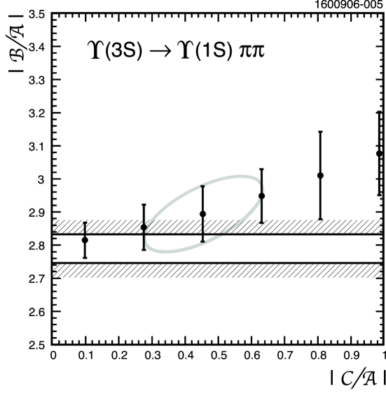
Figure 10: Variation of ${\cal B}$ with ${\cal C}$ magnitudes. The points indicate the fit and error for ${\cal B}$ at fixed values of ${\cal C}$. The ellipse indicates the one sigma bound on the free fit, the axis of which agrees well with the point by point fits. The bands indicate the one standard error limits on ${\cal B}$ when ${\cal C}$ is fixed to zero.

III.4 Partial Wave Decomposition

Since the focus of this study is the decay dynamics of the di-pion system it is useful to think about the spin structure of the di-pion composite. The idea is to look for signatures of higher spin resonances in the form factors ${\cal A}$ and ${\cal B}$. We must account for the intrinsic spin structure of the Lorentz amplitude to do this. We equate the Lorentz amplitude with the general partial wave amplitude to relate the matrix elements.

The transition is of the form $\left<\Upsilon;X|\Upsilon^{\prime}\right>$. If the di-pion system has spin $J$ we have:

$$\left<1,m_{\Upsilon};J_{X},m_{X}|1,m_{\Upsilon^{\prime}}\right>~{}.$$ (7)

In that here we assume that only A and B are non-zero, there is no change in the polarization from the initial state to final state Upsilon; more general partial wave decompositions can also be made CKK ; newVoloshin . The angular momentum projections are then $m_{\Upsilon^{\prime}}=m_{\Upsilon}$, and $m_{X}=0$. Hence the partial wave decomposition of the $X$ system can only have $m=0$ components. Since the pions are in an iso-singlet state, their parities require their relative orbital angular momentum to be even, and hence the orbital angular momentum between the final state upsilon and the di-pion composite must also be even. We can only have even partial waves in our decomposition:

$$\begin{array}[]{rcl}{\cal M}_{P}&=&{\cal S}(q^{2})Y^{0}_{0}+{\cal D}(q^{2})Y^{0}_{2}\\ &=&{\cal S}(q^{2})\frac{1}{\sqrt{4\pi}}+{\cal D}(q^{2})\sqrt{\frac{5}{4\pi}}\left(\frac{3}{2}\cos^{2}\theta_{X}-\frac{1}{2}\right).\end{array}$$ (8)

The functions ${\cal S}(q^{2})$ and ${\cal D}(q^{2})$ are composed of two terms each, one from the ${\cal A}$ dependence and one from the ${\cal B}$ dependence:

$${\cal S}(q^{2})={\cal A}{\cal S}_{{\cal A}}(q^{2})+{\cal B}{\cal S}_{{\cal B}}(q^{2}),\hskip 14.22636pt{\rm and}\hskip 14.22636pt{\cal D}(q^{2})={\cal A}{\cal D}_{{\cal A}}(q^{2})+{\cal B}{\cal D}_{{\cal B}}(q^{2}).$$ (9)

We here assume that there are no significant contributions from partial waves higher than $J=2$. This will be true if there are no contributions from variations of form factors over the Dalitz space. Higher $J$ terms must originate from structure in the form factors ${\cal A}$ and ${\cal B}$.

Equating the decay distributions (or equivalently, projecting inner products over the angular space) yields the following forms:

$${{\cal S}}_{{\cal A}}(q^{2})=q^{2}-2M_{\pi}^{2}~{},\hskip 19.91692pt{\rm and}\hskip 19.91692pt{{\cal D}}_{{\cal A}}(q^{2})=0$$ (10)

for a pure “${\cal A}$” decay, and

$$\begin{array}[]{rcl}{{\cal S}}_{{\cal B}}(q^{2})&=&\frac{q^{2}\left({\left(M_{\Upsilon^{\prime}}^{2}-M_{\Upsilon}^{2}\right)}^{2}+\left(M_{\Upsilon^{\prime}}^{2}+M_{\Upsilon}^{2}\right)q^{2}-2{q^{2}}^{2}\right)+2M_{\pi}^{2}\left({M_{\Upsilon^{\prime}}^{2}}^{2}+{\left(M_{\Upsilon}^{2}-q^{2}\right)}^{2}-2M_{\Upsilon^{\prime}}^{2}\left(M_{\Upsilon}^{2}+q^{2}\right)\right)}{12{\sqrt{M_{\Upsilon^{\prime}}^{2}M_{\Upsilon}^{2}}}q^{2}}~{};\\ {{\cal D}}_{{\cal B}}(q^{2})&=&\frac{\left(4M_{\pi}^{2}-q^{2}\right)\left({M_{\Upsilon^{\prime}}^{2}}^{2}+{\left(M_{\Upsilon}^{2}-q^{2}\right)}^{2}-2M_{\Upsilon^{\prime}}^{2}\left(M_{\Upsilon}^{2}+q^{2}\right)\right)}{12{\sqrt{5}}{\sqrt{M_{\Upsilon^{\prime}}^{2}M_{\Upsilon}^{2}}}q^{2}}\end{array}$$ (11)

for a pure “${\cal B}$” decay. The overall amplitude is

$${\cal M}_{P}=({\cal A}\,{{\cal S}}_{{\cal A}}(q^{2})+{\cal B}\,{{\cal S}}_{{\cal B}}(q^{2}))Y^{0}_{0}+({\cal A}\,{{\cal D}}_{{\cal A}}(q^{2})+{\cal B}\,{{\cal D}}_{{\cal B}}(q^{2}))Y^{0}_{2}~{},$$ (12)

where it is implied that $Y^{m}_{l}$ is a function of the helicity angles of the pseudo-decay $X\rightarrow\pi\pi$, $\theta_{X}$ and $\phi_{X}$ (although the latter variable plays no role in the description of this decay, by the assumptions above). Interference between the $S$-wave and $D$-wave components of the decay comes from the functions ${\cal S}(q^{2})$ and ${\cal D}(q^{2})$ being complex valued. Though ${\cal S}_{{\cal A},{\cal B}}(q^{2})$ and ${\cal D}_{{\cal A},{\cal B}}(q^{2})$ are real functions, ${\cal A}$ and ${\cal B}$ are complex coefficients with nontrivial relative phase.

The structure of $S$ and $D$ components as functions of $q^{2}$ are determined by the assumptions underlying the derivation of the general Lorentz amplitude. The four functions from the pure ${\cal A}$ and pure ${\cal B}$ components are sketched in Fig. 11 together with the fractional $S$- and $D$-wave components in the angular distribution (which can alternately be thought of as the strengths of the $S$- and $D$-wave components), extracted from our fit to $\Upsilon({3}S)\rightarrow\Upsilon({1}S)\pi\pi$.

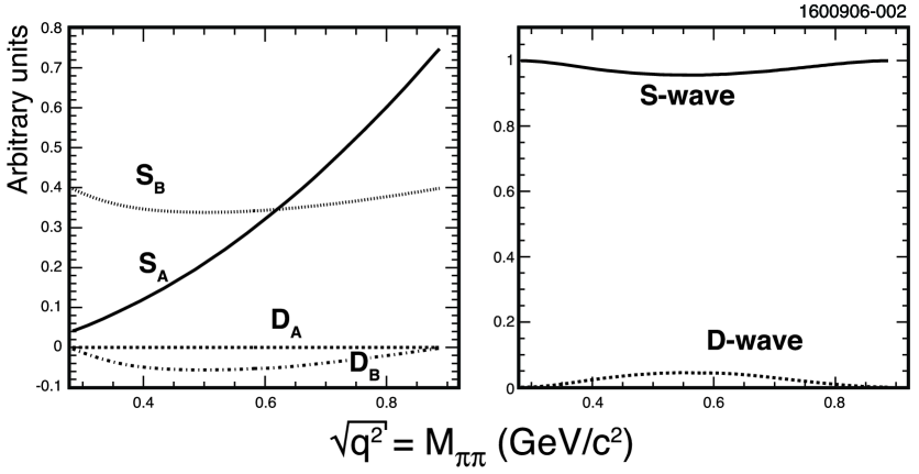
Figure 11: The left plot shows the amplitude component functions ${{\cal S}}_{{\cal A}}$, ${{\cal S}}_{{\cal B}}$, ${{\cal D}}_{{\cal A}}$, and ${{\cal D}}_{{\cal B}}$ as a function of ${M_{\pi\pi}}\equiv\sqrt{q^{2}}$. These are summed to obtain the total amplitude. The partial rate to $S$-wave and $D$-wave components are shown in the right plot for the $\Upsilon({3}S)\rightarrow\Upsilon({1}S)\pi\pi$ decay as determined from the results of this analysis: ${\cal B}/{\cal A}=-2.52+1.19i$. Note that the $D$-wave contribution is largest in the low to intermediate range of $q^{2}$, and is suppressed at both extrema by angular momentum barrier effects. Note further that this is not a resonance phenomenon despite its shape in ${M_{\pi\pi}}$ and the changing angular structure.

This partial wave extraction becomes much more complex if the form factors are assumed to be variable over the Dalitz space, for example due to resonant structure/enhancement in the decay. This will introduce higher powers of $\cos^{2}\theta_{X}$ to the overall amplitude and will need higher partial wave components to account for the variation.

The presence of $D$-wave components in the angular distribution of the decay is not in itself an indication of resonances contributing, nor the presence of unaccounted-for physics. The presence of a $q^{2}$-dependent $D$-wave component could simply be a consequence of angular momentum barriers in the three body phase space of the decay. The data do not demand the introduction of a $q^{2}$-dependent magnitude or phase for ${\cal B}/{\cal B}$. These small $D$-wave components are consistent with those derived in a recent paper by Voloshin Voloshin (2006), in which he emphasizes the importance of relativistic and chromo-magnetic effects.

IV Systematic Uncertainties

We address three sources of systematic uncertainty in the measurements of ${\cal B}/{\cal A}$ and ${\cal C}/{\cal A}$: model dependence, detector efficiency and resolution, and backgrounds.

In Sect. III we showed that our model provides a very good description of the data in the $(q^{2},\cos\theta_{X})$ plane and that the presence or absence of the chromo-magnetic coupled term in the amplitude has little effect on $|{\cal B}/{\cal A}|$ and $\delta_{BA}$.

Uncertainty in the estimation of the detector efficiency and resolution contributes most significantly in the charged mode analyses due to our limited knowledge of the tracking efficiency at very low momentum. In that the low momentum region is precisely where the matrix element has potential suppression in the ${\cal B}$ term, this can potentially cause a significant bias. To estimate this effect we use the full Monte Carlo simulation with looser and tighter track reconstruction requirements to provide bounds on the shape of the efficiency as a function of track curvature. We then create a number of analytic functions that span these boundaries. Then we use a toy Monte Carlo to simulate events with one of these analytic functions and assume a different one for the reconstruction. The variations in the fit results are conservatively assumed to be one standard error uncertainties on the extracted parameters.

The same process is repeated for the neutral modes, varying the thresholds at which showers can be observed in the detector. This obviously leads to a large variation in branching ratios from simple inability to reconstruct the decays, but does not exhibit any significant change in the shape of the efficiency function over the measurement variables. This is to be expected since the $\pi^{0}$ decays have largely flat acceptance over the kinematic range of these decay modes.

We have evaluated the systematic errors associated with detector resolution, and find them to be negligible in comparison with the statistical errors from the fit and the other systematic errors discussed here. The curvatures of the matrix element components across the Dalitz plot are all very much smaller than the variances of the reconstructed measurement variables around their true values. No systematic uncertainty is assigned to this source.

Background subtraction is only a source of bias if the upper and lower sidebands in the recoil mass exhibit markedly different shapes or the background is strongly peaked under the signal. In this case the extrapolations of the background shape and magnitude under the peak could be distorted. We have redone the fits with the ratio of the widths of sideband window to signal window both doubled and halved, and with only using either the high-mass or low-mass sideband. The variations in the fit are conservatively taken to represent one sigma variations in the final result, and are given in the last column of Table 4.

Finally, the lepton reconstruction is capable of contributing bias since all decay modes are fully reconstructed. However, the detector response to leptons is sufficiently well measured in other analyses that the detector simulation is much more precise than what is required for this data set. The variation of the shapes is furthermore only relevant for the final ${\cal C}$ term, which is dependent on the lepton polar angle. With the exception of a small part of the ${\cal C}$ terms there can be no effect due to lepton acceptance. We estimate any systematic error associated with the lepton reconstruction to be negligible.

The fit results combined with these systematic uncertainties are summarized in Tables 4 and 5. Since the magnitude $|{\cal C}/{\cal A}|$ in the fit is only separated from zero by about one standard error and is expected to be suppressed in the theoretical models, we set a limit rather than claim observation of a non-zero value.

We set this limit by assuming the value of ${\cal C}/{\cal A}$ has a Gaussian uncertainty in real and imaginary parts. We transform variables to $|{\cal C}/{\cal A}|$ and $\arg({\cal C}/{\cal A})$, using the sum of the variances of statistical and systematic origin as the overall variance. We then find the 90% upper limit from the resulting distribution as

$$\begin{array}[]{rclcll}|{\cal C}/{\cal A}|&<&1.09&&\rm{at}~{}90\%~{}C.L.~{}.&\end{array}$$ (13)

V Summary and Acknowledgments

We quote fit results for the three transitions from simultaneous fits to the different decay modes with statistical and systematic uncertainties in Table 5. Only the simplest features of the Brown and Cahn decay amplitude (Eqn. 1) are included in our model, and the fits account for the structure of the decay without introduction of new physics or contributions from resonances.

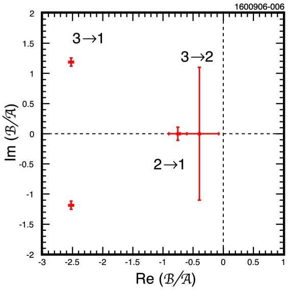
Figure 12: Complex values of matrix element ratio ${\cal B}/{\cal A}$ from combined fits for the three transitions under the assumption that ${\cal C}=0$. Note the two-fold ambiguity in the imaginary part.

The matrix elements are indicated as points in the complex plane in Fig. 12. For the “anomalous” $\Upsilon({3}S)\rightarrow\Upsilon({1}S)\pi\pi$ transition we fit for the presence of the “suppressed” ${\cal C}$ term as a test for the breakdown of the underlying assumptions leading to the standard matrix element. This term is not significant when systematic errors are taken into account and the quality of the fit to the data is good without it. Therefore, we set an upper limit of $|{\cal C}/{\cal A}|<1.09$ at $90\%$ C.L..

We note in particular that the treatment of the di-pion transitions via the full allowed matrix element under the assumptions in Refs.  Brown and Cahn (1975); MBVoloshin:75 ; Gottfried (1978); Yan (1980); Voloshin and Zakharov (1980) allows two matrix elements, only one of which has traditionally been assumed to be non-zero. The description of the $\Upsilon({3}S)\rightarrow\Upsilon({1}S)\pi\pi$ transition di-pion mass and angular structure as anomalous is only true in the limit of this assumption. This analysis shows in particular that the description of the decay process in terms of the two favored amplitude terms, with complex form factors constant over the Dalitz plane, suffices to describe the decay distributions of $\Upsilon({3}S)\rightarrow\Upsilon({1}S)\pi\pi$, $\Upsilon({3}S)\rightarrow\Upsilon({2}S)\pi\pi$, and $\Upsilon({2}S)\rightarrow\Upsilon({1}S)\pi\pi$, provided the form factors are allowed to vary with the transition. For the $\Upsilon$(3S)$\to\Upsilon$(1S)$\pi\pi$ transition, we find $|{\cal B}/{\cal A}|=2.79\pm 0.05$, which could imply a large magnitude of ${\cal B}$ or a suppressed ${\cal A}$; recent theoretical considerations Voloshin (2006) favor the latter interpretation. While smaller than in the case of $\Upsilon({3}S)\rightarrow\Upsilon({1}S)\pi\pi$, $|{\cal B}/{\cal A}|$ is also determined to be non-zero for the case of $\Upsilon({2}S)\rightarrow\Upsilon({1}S)\pi\pi$. The large imaginary part of ${\cal B}/{\cal A}$ is intriguing newVoloshin .

While there are not yet first principles predictions of the values of the matrix elements of the decays studied here, this analysis does provide complete measurements of the relative matrix element magnitudes and phases that can serve as a point of comparison with ab initio QCD calculations.

Fit, No ${\cal C}$ stat. effcy. ($\pi^{\pm}$) effcy.($\pi^{0}$) bg. sub. $\Upsilon({3}S)\rightarrow\Upsilon({1}S)\pi\pi$ $\begin{array}[]{c}\Re({\cal B}/{\cal A})\\ \Im({\cal B}/{\cal A})\end{array}$ $\begin{array}[]{r}-2.523\\ \pm 1.189\end{array}$ $\begin{array}[]{l}\pm 0.031\\ \pm 0.051\end{array}$ $\begin{array}[]{l}\pm 0.019\\ \pm 0.026\end{array}$ $\begin{array}[]{l}\pm 0.011\\ \pm 0.018\end{array}$ $\begin{array}[]{l}\pm 0.001\\ \pm 0.015\end{array}$ $\Upsilon({2}S)\rightarrow\Upsilon({1}S)\pi\pi$ $\begin{array}[]{c}\Re({\cal B}/{\cal A})\\ \Im({\cal B}/{\cal A})\end{array}$ $\begin{array}[]{r}-0.753\\ 0.000\end{array}$ $\begin{array}[]{l}\pm 0.064\\ \pm 0.108\end{array}$ $\begin{array}[]{l}\pm 0.059\\ \pm 0.036\end{array}$ $\begin{array}[]{l}\pm 0.035\\ \pm 0.012\end{array}$ $\begin{array}[]{l}\pm 0.112\\ \pm 0.001\end{array}$ $\Upsilon({3}S)\rightarrow\Upsilon({2}S)\pi\pi$ $\begin{array}[]{c}\Re({\cal B}/{\cal A})\\ \Im({\cal B}/{\cal A})\end{array}$ $\begin{array}[]{r}-0.395\\ \pm 0.001\end{array}$ $\begin{array}[]{l}\pm 0.295\\ \pm 1.053\end{array}$ $\begin{array}[]{r}\pm 0.025\\ \pm 0.180\end{array}$ $\begin{array}[]{l}\pm 0.120\\ \pm 0.001\end{array}$ Fit, float ${\cal C}$ stat. effcy. ($\pi^{\pm}$) effcy.($\pi^{0}$) bg. sub. $\Upsilon({3}S)\rightarrow\Upsilon({1}S)\pi\pi$ $\begin{array}[]{c}|{\cal B}/{\cal A}|\\ |{\cal C}/{\cal A}|\end{array}$ $\begin{array}[]{r}2.89\\ 0.45\end{array}$ $\begin{array}[]{l}\pm 0.11\\ \pm 0.18\end{array}$ $\begin{array}[]{l}\pm 0.19\\ \pm 0.28\end{array}$ $\begin{array}[]{l}\pm 0.11\\ \pm 0.20\end{array}$ $\begin{array}[]{l}\pm 0.027\\ \pm 0.093\end{array}$

Table 4: Combined fit results for all transitions with statistical and systematic uncertainties. The systematic uncertainties are in order: $\pi^{\pm}$ detection efficiency, $\pi^{0}$ detection efficiency, and background subtraction for the $\Upsilon({3}S)\rightarrow\Upsilon({2}S)\pi\pi$ transition. The upper set of results are for the fits assuming contributions to the amplitude from only the ${\cal A}$ and ${\cal B}$ terms. The bottom two lines are the fit results when the ${\cal C}$ term is allowed to be non-zero. The imaginary part of the ratio has a two-fold ambiguity and is only known to within a sign. Note that for the transition $\Upsilon({3}S)\rightarrow\Upsilon({2}S)\pi\pi$ we do not have fits for the charged di-pion case.

Fit, no ${\cal C}$, total error $\Upsilon({3}S)\rightarrow\Upsilon({1}S)\pi\pi$ $\begin{array}[]{c}\Re({\cal B}/{\cal A})\\ \Im({\cal B}/{\cal A})\\ |{\cal B}/{\cal A}|\\ \delta_{BA}\end{array}$ $\begin{array}[]{rcl}-2.52&\pm&0.04\\ \pm 1.19&\pm&0.06\\ 2.79&\pm&0.05\\ 155(205)&\pm&2\end{array}$ $\Upsilon({2}S)\rightarrow\Upsilon({1}S)\pi\pi$ $\begin{array}[]{c}\Re({\cal B}/{\cal A})\\ \Im({\cal B}/{\cal A})\\ |{\cal B}/{\cal A}|\\ \delta_{BA}\end{array}$ $\begin{array}[]{rcl}-0.75&\pm&0.15\\ 0.00&\pm&0.11\\ 0.75&\pm&0.15\\ 180&\pm&9\end{array}$ $\Upsilon({3}S)\rightarrow\Upsilon({2}S)\pi\pi$ $\begin{array}[]{c}\Re({\cal B}/{\cal A})\\ \Im({\cal B}/{\cal A})\end{array}$ $\begin{array}[]{rcl}-0.40&\pm&0.32\\ 0.00&\pm&1.1\end{array}$ Fit, float ${\cal C}$, total error $\Upsilon({3}S)\rightarrow\Upsilon({1}S)\pi\pi$ $\begin{array}[]{c}|{\cal B}/{\cal A}|\\ |{\cal C}/{\cal A}|\end{array}$ $\begin{array}[]{rcl}2.89&\pm&0.25\\ 0.45&\pm&0.40\end{array}$

Table 5: Fit results for all transitions with total uncertainties. These numbers represent the final result of this analysis. In the case of the magnitude ratio $|{\cal C}/{\cal A}|$, we also quote a limit as detailed in the text. The phase angles are quoted in degrees, and have a two-fold ambiguity of reflection in the real axis.

We gratefully acknowledge the effort of the CESR staff in providing us with excellent luminosity and running conditions. D. Cronin-Hennessy and A. Ryd thank the A.P. Sloan Foundation. This work was supported by the National Science Foundation, the U.S. Department of Energy, and the Natural Sciences and Engineering Research Council of Canada.

VI Appendix: Details of the Likelihood Fitter

This appendix gives some details of our application of the likelihood fitter.

Smearing due to reconstruction resolution adds a small variance to the Poisson error on the Monte Carlo integral, but the smearing widths are small compared to the scales over which the matrix element changes so this additional variance is small. For any shape with an approximately polynomial form at a point, the resolution is described by convolving a Gaussian with the polynomial. As an example, we assume a functional form $g^{T}=a+b\,x+c\,x^{2}$ and seek its observed shape in terms of the observed variables, $g^{O}(x^{O})$, using a Gaussian transformation:

$$g^{O}(x^{O}) = \int dx^{T}{\cal G}(x^{T}-x^{O}|\mu\equiv 0,\sigma)g^{T}(x^{T})$$ (14)

$$= \int dx^{T}{\cal G}(x^{T}-x^{O}|\mu\equiv 0,\sigma)(a+b\,x^{T}+c\,(x^{T})^{2})$$ (15)

$$= (a+c\,\sigma^{2})+b\,x^{O}+c\,(x^{O})^{2}$$ (16)

So long as $\sigma^{2}\ll a/c$, i.e., the resolution is small compared to the curvature, the shape will not be materially changed. For the angular dependence, which is quartic in $\cos\theta_{X}$ this means the resolution need only be small compared to 1/2; the observed resolutions are of the order of 5% or less. In ${M_{\pi\pi}}$ the same holds true, with the scale being given by the pion mass, $140\,{\rm{\rm MeV}/c^{2}}$, and the observed resolutions being at worst $10\,{\rm{\rm MeV}/c^{2}}$. The shape of the decay amplitude is not changed significantly by these resolutions, but any residual effect is included in the estimated tracking and shower systematic uncertainties.

Our problem differs from that discussed in Ref. Barlow and Beeston (1993) in that the templates do not have independent Poisson fluctuations. The underlying phase space simulation has a Poisson fluctuation, but the templates are known (very nearly) exactly and uncertainties on them do not contribute to the overall likelihood function.

In the absence of background this problem is solved as follows, with each two-dimensional ($q^{2}$, cos$\theta_{X}$) bin denoted by subscript $i$.

We compare the Monte Carlo simulated, acceptance and efficiency-corrected, phase space distribution (with true and observed yields $A_{i}$ and $a_{i}$), multiplied by the modulus squared of the amplitude, with the data distribution (with true and observed yields $D_{i}$ and $d_{i}$). Both distributions are subject to Poisson fluctuation:

$${\cal P}(d_{i};D_{i})=\frac{e^{-D_{i}}{D_{i}}^{d_{i}}}{d_{i}!}\hskip 14.22636pt\mbox{and}\hskip 14.22636pt{\cal P}(a_{i};A_{i})=\frac{e^{-A_{i}}{A_{i}}^{a_{i}}}{a_{i}!}.$$ (17)

Bin-by-bin, the modulus squared of the decay amplitude appears in the exact relation between the true data yields $D_{i}$ and the true phase space yields $A_{i}$:

$$D_{i}=f_{i}(\alpha)\,A_{i}.$$ (18)

The function $f_{i}$ represents the decay distribution ($|{\cal M}|^{2}$) in the kinematic space bin $i$ as a function of $\alpha$, the decay parameters. In this case $\alpha$ consists of real and imaginary parts of ${\cal B}/{\cal A}$ and ${\cal C}/{\cal A}$.

The log likelihood used in this fit is then given by, summing over all the bins:

$$\ln{\cal L}(\alpha)=\sum_{i=1}^{n}\left(d_{i}\ln{f_{i}(\alpha)A_{i}}-f_{i}(\alpha)A_{i}-\ln{d_{i}!}+a_{i}\ln{A_{i}}-A_{i}-\ln{a_{i}!}\right).$$ (19)

The $A_{i}$ represent the phase space subject to efficiency and acceptance effects and are uninteresting nuisance parameters that can be eliminated by extremizing the likelihood with respect to them. Proceeding in analogy with the approach in Barlow and Beeston (1993) we can find the analytic extremum condition, solve for $A_{i}$

$$A_{i}=\frac{d_{i}+a_{i}}{f_{i}+1}$$ (20)

and substitute back into the likelihood function to give a reduced likelihood:

$$\ln{\cal L}(\alpha)=\sum_{i=1}^{n}\left[\rule{0.0pt}{16.0pt}d_{i}\ln f_{i}(\alpha)-(d_{i}+a_{i})\ln(1+f_{i}(\alpha))\right]+{\rm const.}$$ (21)

We then minimize $-2\ln{\cal L}$ with respect to the fit parameters $\alpha$ (occurring only in the coefficients $f_{i}$). This is implemented using the CERN Library minimization package, MINUIT James (1998).

The full likelihood as used in the fit includes an extension of this approach to account for background under the signal peaks. This introduces additional parameters $B_{i}$ and $b_{i}$. These represent bin by bin true and observed background yields. The $B_{i}$ are a second set of nuisance parameters that are eliminated in the same way as were the $A_{i}$ before. The resulting likelihood is significantly more complicated in detail but not in principle. For brevity it is not included here.

References

- (1) A. Rittenberg, UCRL-18863, Ph.D. Thesis (unpublished), 1969; G. W. London et al., Phys. Rev. 143, 1034 (1966); J. Badier et al., Phys. Lett. 17, 337 (1965).
- (2) T. M. Himel, Ph.D. Thesis, SLAC-223 (1979); M. Oreglia et al. (Crystal Ball Collaboration), Phys. Rev. Lett. 45, 959 (1980); H. Albrecht et al. (ARGUS Collaboration), Zeit. für Phys. C35, 283 (1987); J. Z. Bai et al. (BES Collaboration), Phys. Rev. D62, 032002 (2000).
- Brown and Cahn (1975) L. S. Brown and R. N. Cahn, Phys. Rev. Lett. 35, 1 (1975).
- (4) M. B. Voloshin, P. Zh. Eksp. Fiz. 21, 733 (1975) [JETP Lett., 21, 347 (1975)].
- Butler et al. (1994) F. Butler et al. (CLEO Collaboration), Phys. Rev. D49, 40 (1994).
- Glenn et al. (1999) S. Glenn et al. (CLEO Collaboration), Phys. Rev. D59, 052003 (1999).
- Alexander et al. (1998) J. P. Alexander et al. (CLEO Collaboration), Phys. Rev. D58, 052004 (1998).
- Brock et al. (1991) I. C. Brock et al. (CLEO Collaboration), Phys. Rev. D43, 1448 (1991).
- (9) G. Belanger, T. DeGrand and P. Moxhay, Phys. Rev. D39, 257 (1989).
- (10) S. Chakravarty, S. M. Kim and P. Ko, Phys. Rev. D50, 389 (1994).
- (11) T. Komada, S. Ishida and M. Ishida, Phys. Lett. B 508, 31 (2001); Phys. Lett. B 518, 47 (2001).
- (12) M. Uehara, Prog. Theor. Phys. 109, 265 (2003).
- (13) M. B. Voloshin, P. Zh. Eksp. Fiz. 37, 58 (1983) [JETP Lett. 37, 69 (1983)].
- (14) V. V. Anisovich, D. V. Bugg, A. V. Sarantsev and B. S. Zhou, Phys. Rev. D51, 4619 (1995).
- (15) F.-K. Guo, P.-N. Shen, H.-C. Chiang and R.-G. Ping, Nucl. Phys. A 761, 269 (2005).
- (16) P. Moxhay, Phys. Rev. D39, 3497 (1989).
- (17) H. J. Lipkin and S. F.Tuan, Phys. Lett. B 206, 349 (1988).
- (18) H.-Y. Zhou and Y-P. Kuang, Phys. Rev. D44, 756 (1991).
- (19) S. Chakravarty, S. M. Kim and P. Ko, Phys. Rev. D48, 1212 (1993).
- Voloshin (2006) M. B. Voloshin, Phys. Rev. D74, 054022 (2006).
- Abe et al. (2005) K. Abe et al. (BELLE Collaboration) (2006), eprint hep-ex/0611026.
- (22) B. Aubert et al. (aar Collaboration), Phys. Rev. Lett. 96, 232001 (2006).
- Gottfried (1978) K. Gottfried, Phys. Rev. Lett. 40, 598 (1978).
- Yan (1980) T. M. Yan, Phys. Rev. D22, 1652 (1980).
- Voloshin and Zakharov (1980) M. B. Voloshin and V. I. Zakharov, Phys. Rev. Lett. 45, 688 (1980).
- (26) T. Mannel and R. Urech, Z. Phys. C73, 541 (1997).
- (27) S. Dubynskiy and M. B. Voloshin, arXiv:0707.1272.
- Viehhauser (2001) G. Viehhauser, Nucl. Instrum. Meth. A462, 146 (2001).
- Peterson et al. (2002) D. Peterson et al., Nucl. Instrum. Meth. A478, 142 (2002).
- Artuso et al. (2005) M. Artuso et al., Nucl. Instrum. Meth. A554, 147 (2005).
- Yao et al. (2006) W.-M. Yao et al. (Particle Data Group), Jour. of Physics G 33, 1 (2006).
- (32) T. Sjostrand et al., Comput. Phys. Commun. 135, 238 (2001); for more details see T. Sjostrand, L. Lonnblad and S. Mrenna, PYTHIA 6.2 Physics and Manual, hep-ph/0108264.
- (33) See http://w4.lns.cornell.edu/public/CLEO/soft/QQ/index.html.
- CER (1993) GEANT: Detector Description and Simulation Tool, CERN (1993), long writeup W5013.
- Barlow and Beeston (1993) R. J. Barlow and C. Beeston, Comput. Phys. Commun. 77, 219 (1993).
- James (1998) F. James, MINUIT: Function Minimization and Error Analysis, CERN (1998), long writeup D506.