Carrier-carrier entanglement and transport resonances in semiconductor quantum dots

Abstract

We study theoretically the entanglement created in a scattering between an electron, incoming from a source lead, and another electron bound in the ground state of a quantum dot, connected to two leads. We analyze the role played by the different kinds of resonances in the transmission spectra and by the number of scattering channels, into the amount of quantum correlations between the two identical carriers. It is shown that the entanglement between their energy states is not sensitive to the presence of Breit-Wigner resonances, while it presents a peculiar behavior in correspondence of Fano peaks: two close maxima separated by a minimum for a two-channel scattering, a single maximum for a multi-channel scattering. Such a behavior is ascribed to the different mechanisms characterizing the two types of resonances. Our results suggest that the production and detection of entanglement in quantum dot structures may be controlled by the manipulation of Fano resonances through external fields.

I Introduction

Quantum entanglement, as one of the most spectacular features of quantum mechanics contrasting with classical physics Eins , has been widely investigated in the last decades, mainly because it is recognized as a crucial resource for quantum information processing and quantum communication Bouwn . It is therefore a problem of great interest to find physical systems where the entanglement can be produced, manipulated and detected. Recently there have been different proposals to produce entangled states, such as those based on atomic systems chan , quantum electrodynamics cavities Lof and solid state devices bus ; berbor ; bor2 ; Oli ; raa ; Rasm . Among the systems proposed for the realization of quantum information processing devices, those constructed with semiconductor quantum dots (QDs) are extremely promising due mainly to the controllability of their quantum state Div ; Ima ; Zun . Indeed, semiconductor QDs posses many desirable features: an atomic-like structure, that can be fully controlled by an external electrostatical potential; a tunable coupling to source and drain leads, which makes feasible the integration with other microelectronics devices; and the scalability, which seems to promise sophisticate engineering of the multi-QD structures.

QDs represent also an ideal laboratory to compare exact numerical simulations of the quantum transport phenomena with experiments, since the number of degrees of freedom involved is often small and the discreteness of QD states highly reduces the computational burden needed. Various effects such as the conductance quantization Been , the Coulomb blockade due to the electron repulsion Meira , the interplay between resonances and the charging in QD structures Wiel ; Lasse , strongly affect the transport properties. Another peculiar feature of the electron transmission through QDs is the partial retention of quantum coherence Aik , whose measurement, by experimental setups exploiting quantum interference (e.g. with a QD embedded in an Aharonov-Bohm interferometer), may yield information about transport phenomena, not readily available from conductance measures Heib1 ; Heib2 ; Heib3 .

In the frame of quantum transport in semiconductors, theoretical and experimental investigations have revealed other mechanisms governing the electronic transmission through QD structures. In particular it has been observed that two kinds of resonances can be present in conductance spectra, known as Fano and Breit-Wigner resonances Gor ; Fuh ; Lad ; Berton ; Noc . The formers are present when two transmission channels, a resonant one and a non-resonant one, interfere Fano . Moreover they exhibit typical asymmetrical line shapes, with the transmitted phase increasing by $\pi$ on the resonance peak and then dropping abruptly. The latters show a symmetric line shape and may be considered a limiting case of Fano resonances, occurring, for example, when there is a single channel Breit .

In this paper we address the problem of entanglement generation in a two-particle scattering in a QD structure. We analyze, in particular, the role played by some mechanisms of charge transport in the appearance of quantum correlations. To this aim we consider a scattering event in a one-dimensional (1D) double-barrier resonant tunnelling device (that mimics the confining potential of the QD), with an electron incoming from one lead and another electron bound in the ground state of the QD. The two particles feel the confining potential inside the device and interact through the Coulomb repulsion. Indeed carrier-carrier entanglement has been recently investigated in various QD structures Oli ; raa ; Tam ; Ryc ; Contre ; inn ; Lopez where different scattering setups are considered for the generation of two-electron entangled states. In the present work, we adopt a time-independent few-particle approach that, although computational demanding, can be solved numerically to obtain the exact modulus and phase of the transmission coefficient (TC) of an electron crossing the charged QD. This gives us the possibility to quantify the quantum correlation between the energy states of the scattered electron and the bound one, and to expose its connection with the resonances exhibited by the TCs of the various scattering channels. Unlike previous works Oli ; Lopez , the few-particle approach we use in this paper allows us to study the relation between the different kinds of resonances, or the number of energy levels available, with the entanglement formation. Even if the dynamics of carriers has been considered as 1D, we can assume that the results obtained describe a general behavior concerning also quantum transport in 2D and 3D physical systems, being the appearance of quantum correlations closely related to the nature of transport resonances, whose underlying mechanisms are independent from the dimensionality of the system.

The paper is organized as follow. In Sec. II we describe the physical model and the numerical approach adopted to calculate the two-particle scattering state and the quantum correlations in terms of the von Neumann entropy. In Sec. III we present the numerical results obtained for the entanglement in the case of two different kinds of processes, namely two- and multi-channel scattering . Finally in Sec. IV we comment the results, draw final remarks and point out issues that require further research.

II THE PHYSICAL MODEL AND THE NUMERICAL APPROACH

Our aim is to evaluate the entanglement between the energy states of two electrons, interacting via the Coulomb potential, one bound in a QD and the other passing through it. Here we summarize the physical model adopted for the open QD and the numerical approach used to evaluate the two-particle scattering state and the entanglement.

We consider a quasi 1D double-barrier resonant tunnelling device as, for example, the ones formed by material modulation in a ultrathin cylindrical nanowire Bjork . The transversal dimensions of the structure are small compared to the other lenghtscales so that a single transversal subband is accessible to the carriers and the effective dynamics can be considered 1D Fogler . Two small potential barriers separate the QD region from the two contacts, as depicted in Fig. 1(a). The $N$ bound states and energies of the QD will be indicated as $\chi_{n}$ and $E_{n}$ (with $n=0,1,\dots,N$ in order of increasing energy), respectively.

A single electron is in the QD ground state $\chi_{0}$, whereas a second electron is incoming from the left lead with energy $E_{IN}$, and it is scattered by the structure potential $V_{s}$ and by the Coulomb interaction with the bound particle. The potential $V_{s}$ is supposed to be constant outside the region of interest of length $\Delta$ and, without loss of generality, it is taken to be zero in both left and right contacts. We will consider only cases in which the energy of the incoming electron is not sufficient to ionize the QD, i.e. $(E_{IN}+E_{0})<0$. This means that when an electron leaves the scattering region, either reflected or transmitted, the other one is in a bound state of the dot.

The two-particle Hamiltonian reads:

$${\bf H}(x_{1},x_{2})=-\frac{\hbar^{2}}{2m^{*}}\nabla^{2}_{1}-\frac{\hbar^{2}}{2m^{*}}\nabla_{2}^{2}$$ (1)

$$+V_{s}(x_{1})+V_{s}(x_{2})+\frac{e^{2}}{4\pi\epsilon\sqrt{\left(x_{1}-x_{2}\right)^{2}+d^{2}}}\ ,$$

where $m^{*}$ and $\epsilon$ are the electron effective mass and the dielectric constant of the material, respectively. In particular the calculations presented in this paper have been performed using GaAs material parameters. The Coulomb term includes the thickness a cut-off term $d$ that can be assumed to correspond roughly to the lateral dimension of the confinement Fogler . The spin degree of freedom does not enter into our calculation since we neglect spin-orbit coupling . As a consequence of the fermionic nature of the system we impose antisymmetrization constraints under particle exchange to the wavefunction $\psi(x_{1},x_{2})$. This is done by adopting antisymmetric boundary conditions as briefly described in the following and detailed in Ref. Berton, .

The two-particle scattering state is obtained by solving the time-independent open-boundary Schrödinger equation ${\bf H}\psi=E\psi$ in the 2D domain of interest. To this aim we have used a numerical approach, based on a generalization of the widely used quantum transmitting boundary method Lent . It allows us to include proper open boundary conditions and simulate the scattering of one electron by a charge confined in a QD Berton . In particular here we need four boundary conditions, one for each edge of the square domain. Since we have to impose exchange symmetry to $\psi(x_{1},x_{2})$, they are equal in couples, apart from the sign. In fact the form of the wavefunction when particle $1$ is in the left lead ($x_{1}<0$) is

$$\psi(x_{1},x_{2})|_{(x_{1}<0)}=\chi_{0}(x_{2})e^{ik_{0}x_{1}}+$$ (2)

$$+\sum_{n=0}^{M}b_{n}\chi_{n}(x_{2})e^{-ik_{n}x_{1}}\sum_{n={M}+1}^{\infty}b_{n}\chi_{n}(x_{2})e^{k_{n}x_{1}},$$

and, when it is particle $2$ the one in the left lead, the boundary condition is $\psi(x_{1},x_{2})|_{(x_{2}<0)}=-\psi(x_{2},x_{1})|_{(x_{2}<0)}$. For the other two boundaries, namely the conditions ($x_{1}>\Delta$) and ($x_{2}>\Delta$) it holds

$$\psi(x_{1},x_{2})|_{(x_{1}>\Delta)}=$$

$$\sum_{n=0}^{M}c_{n}\chi_{n}(x_{2})e^{ik_{n}x_{1}}+\sum_{n={M}+1}^{\infty}c_{n}\chi_{n}(x_{2})e^{-k_{n}x_{1}}$$ (3)

and $\psi(x_{1},x_{2})|_{(x_{2}>\Delta)}=-\psi(x_{2},x_{1})|_{(x_{2}>\Delta)}$, respectively.

Let us now describe the above expressions. We first define $T_{n}=E_{IN}+E_{0}-E_{n}$ as the energy of an electron freely propagating in the lead when the other one is bound in $\chi_{n}$ (a consequence of energy conservation), and $k_{n}=\sqrt{2m^{*}|T_{n}|}/\hbar$. The right hand side of Eq. (2) (for the left boundary) is the sum of three terms. The first one represents an electron incoming as a plane wave with energy $E_{IN}=\hbar^{2}k_{0}^{2}/2m^{*}$, while the other electron is in the QD ground state $\chi_{0}$. The second term accounts for all the energy-allowed possibilities with one electron bound in the $\chi_{n}$ state, and the other one reflected in the left lead, with wave vector $k_{n}$. $M$ is the number of states for which $T_{n}$ is positive. The third term accounts for the cases $T_{n}<0$, representing the electron in the lead as an evanescent wave. The right hand side of Eq. (II) (for the right boundary) has only two terms, since the probability amplitude of a carrier incoming from the right lead is zero in our system. The first term represents the $M$ energy-allowed possibilities of an electron transmitted and freely propagating in the right lead and the second term includes the outgoing-particle evanescent waves, as in Eq. (2). The reflection and transmission amplitudes in the various energy levels, $b_{n}$ and $c_{n}$ respectively, are unknowns and are obtained by solving the Schrödinger equation with ${\bf H}(x_{1},x_{2})$ given by Eq. (1) and with the two-particle energy $E=E_{IN}+E_{0}$, imposing the two boundary conditions of Eqs. (2) and (II).

In order to describe the mechanisms characterizing the charge transport through a QD, and the kind of resonances showing up in transmission spectra, we report in Fig. 1 the modulus and phase of the TC as a function of the initial energy of the incoming electron, for a given configuration of the potential sketched in the panel (a). In particular we consider a width $L$ of the potential well of 80 nm with a depth $h$ of 150 meV. In this case we have a single-channel scattering, i.e. the scattered particle can have a single energy, while the bound one is always left in the ground state of the QD well. When $E_{IN}$ is around 1.5 meV, the TC shows a Breit-Wigner resonance, as shown in panel (b)Breit . As it is well known, such kinds of resonances stem from the coupling of a quasi-bound state to the scattering states in the leads and presents a Lorentzian line-shape whose amplitude $c_{0}$ is described by the expression $c_{0}=C(i\Gamma/2)/(E_{IN}-E_{qb}+i\Gamma/2)$, where $C$ is a complex constant, $\Gamma$ the width of the resonance, inversely proportional to the lifetime of the quasi-bound state with energy $E_{qb}$. In particular, as we can see from Fig. 1(b), the TC modulus (solid line) goes to 1 with a symmetric Lorentzian peak around the energy resonance, while the transmission phase (dashed line) smoothly changes by $\pi$. In addition to the above resonance two extremely sharp resonances for $E_{IN}$ around 0.3 meV and 0.6 meV, are present. They are the so-called Fano resonances (with asymmetric line-shape), which can be ascribed to an effect brought about by electron-electron correlation Fano . In fact they originated from the interference between a resonant mechanism, due to the Coulomb blockade in the QD, and a non-resonant mechanism, given by the transmission in the dot via a direct trajectory Fuh ; Berton . In order to give a better insight into their properties we have reported in the top panel (c) a zoom of the modulus and phase of the TC at an initial energy of the incoming electron $E_{IN}$ around 0.3 meV. Here the modulus reaches 1 and then goes to zero, showing the typical asymmetric Fano lineshape. The transmission phase increases smoothly by $\pi$ on the resonance peak, but shows an abrupt drop of $\pi$ in correspondence of the zero of the transmission probability bertoni2 . We stress that the curves in Fig. 1 correspond to a single-channel two-particle scattering, with the energy of the transmitted electron fixed by the boundary conditions. As a consequence, no entanglement is generated between the two electrons here. The more interesting cases of two- and multi-channel scattering will be presented in the following section.

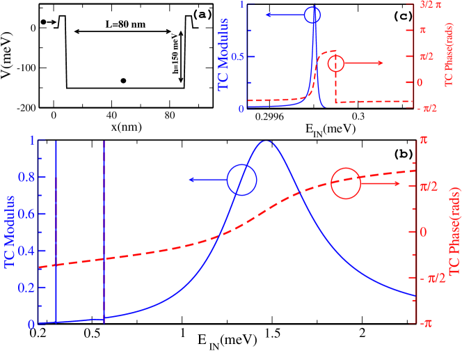
Figure 1: (Color online) Bottom panel (b): TC as a function of the initial energy of the incoming electron $E_{IN}$. The solid line represents the modulus of the TC and refers to the left ordinate axis; the dashed line represents the phase of TC and refers to the right axis. Top panels: (a) profile of the potential $V(x)$ in the scattering region: the potential well is 150 meV deep and 80 nm wide and is connected to the leads through two 10 nm barriers of 30 meV; (c) zoom of the TC modulus and phase for $E_{IN}\simeq 0.3$ meV where a Fano resonance occurs.

In the last part of this section we describe the procedure we adopt to evaluate the entanglement. In fact as a consequence of the scattering, quantum correlations appear between the energy levels $E_{n}$ of the electron bound in the potential well and the energies $T_{n}$ of the scattered electron allowed by energy conservation. Such an entanglement may be evaluated from the transmitted component of the two-particle wavefunction in the right lead, given by Eq. (II). Obviously only the travelling components, with $n\leq M$ in the right hand side of Eq. (II), must be considered, since they are the only ones giving a non vanishing contribution to the current and also the only ones that could be revealed by measuring the energy of the electron propagating in the right lead. On the other hand the evanescent component of the wavefunction plays no direct role in the appearance of detectable quantum correlations. In this case, a good entanglement measure is given by the von Neumann entropy of the reduced density matrix $\rho_{Red}$, obtained by tracing the two-particle density matrix $\rho=|\Psi^{tr}\rangle\langle\Psi^{tr}|/\langle\Psi^{tr}|\Psi^{tr}\rangle$ over the degrees of freedom of one of the particles Peres , where $\psi(x_{1},x_{2})^{tr}=\sum_{n=0}^{M}c_{n}\chi_{n}(x_{2})e^{ik_{n}x_{1}}$.

$\rho_{Red}$ will be a $(M+1)\times(M+1)$ diagonal matrix defined as

$$\rho_{Red}=\textrm{diag}\bigg{[}|\widetilde{c}_{0}|^{2},\ldots,|\widetilde{c}_{n}|^{2},\ldots,|\widetilde{c}_{M}|^{2}\bigg{]}$$ (4)

with

$$\widetilde{c}_{n}=\frac{c_{n}}{\sqrt{\sum_{n=0}^{M}|c_{n}|^{2}}}.$$ (5)

Thus the entanglement can be expressed by means of the von Neumann entropy as

$$\varepsilon=-\textrm{Tr}\left[\rho_{Red}\ln{\rho_{Red}}\right]=-\sum_{n=0}^{M}|\widetilde{c}_{n}|^{2}\ln{|\widetilde{c}_{n}|^{2}}.$$ (6)

$\varepsilon$ is bound in the interval $\left[0,\ln{\left(M+1\right)}\right]$ with $\varepsilon=0$ indicating no entanglement and $\varepsilon=\ln{\left(M+1\right)}$ indicating a maximally-entangled state. We stress that, unlike other works estimating the quantum correlation in QDs Oli ; Lopez , we are not considering the transmitted and reflected component of the scattering wavefunction as two different states that can be entangled with the QD. We estimate the entanglement between the dot and the transmitted electron. In fact, in our approach the measure of the entanglement created in the system, evaluated by means of Eq. (6), is not explicitely given in terms of the device transmission and reflection coefficients, but it is a function of the amplitude probabilities of finding the transmitted particle in one of the possible energy states. Furthermore, it is worth noting that, although we do not use explicitely the criteria developed to treat the entanglement of identical particles Sch ; bus ; bus2 , the electrons in our system are fully indistinguishable. Nevertheless, since the energy of the incoming electron is not sufficient to ionize the QD, we may safely assume that the scattered particle is far enough from the one left in a bound state of the dot so that the overlap between their spatial probabilities is negligible. In other words we use the spatial position of the electrons to “distinguish” them, while the entanglement is between their energy states, as suggested in Ref. eck, .

III Numerical results

In this section we analyze the entanglement formation in a two- or multi-channel scattering, and its relation to the resonances in the TCs. In particular, it is of interest to study how the entanglement depends upon the kind of resonances, since the detection of the latter, usually feasible through a current-voltage characteristic of the quantum device, can give information about the former. In our approach we solve numerically the system for different potentials $V(x)$ (obtained by varying the depth $h$ and the width $L$ of the well), and for different initial energies of the incoming electron $E_{IN}$.

In panel (a) of Fig. 2 we report the entanglement $\varepsilon$ of the system as a function of the initial energy of the incoming electron and of the depth of the potential well, whose width is kept constant at $L$= 40 nm. The entanglement presents extremely sharp peaks that, as we shall see, correspond to the resonances exhibited by the TCs of the various channels. From the 2D representation of the same data, displayed in Fig. 2(b), we observe that the maxima of the entanglement spread in the region corresponding to a three-channel scattering, that is separated by the dashed line from the one where the number of active channels is two. This suggests us that also the kind of process, i.e. two- or multi-channel scattering, plays an important role into the entanglement formation. The two cases will be better analyzed in the following subsections.

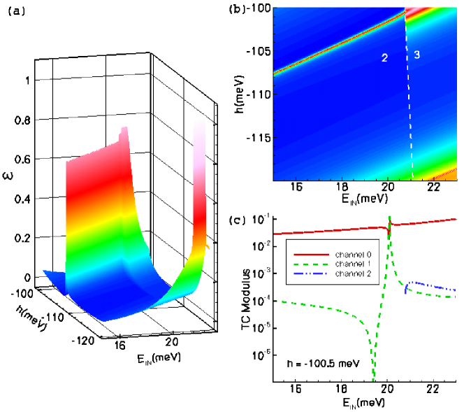
Figure 2: (Color online) Left panel (a): entanglement $\varepsilon$ as a function of the initial energy of the incoming electron $E_{IN}$ and of the depth of the potential well of 40 nm. Right panels: (b) 2D contour plot of the same data; the dashed line is a guide for the eyes and separates the zone corresponding to two-channel scattering (left) from the one corresponding to a three-channel scattering (right); (c) modulus of TC of the three channels as a function of $E_{IN}$ with $h$ fixed at 100.5 meV. Note that the channel 2 is activated only at $E_{IN}\simeq 21$ meV.

III.1 Two-Channel scattering

Here we study the creation of the entanglement when the incident particle, as a consequence of the scattering with the particle bound in the QD, is transmitted with two possible energies, $T_{0}$ and $T_{1}$, and, correspondingly, the final QD energy can be $E_{0}$ and $E_{1}$.

In the top panel of Fig. 3 we report the entanglement as a function of the kinetic energy of the incoming particle, for the potential sketched in the inset of the figure. In particular we consider a width of the potential well of 30 nm and a depth of $110$ meV. At low energies the scattering does not lead to the appearance of quantum correlations between the two particles, since only a single channel is possible for the transmission. It is therefore possible to attribute a specific energy to each particle: $T_{0}$ for the scattered electron and $E_{0}$ for the bound one. When $E_{IN}$ reaches a threshold value of about 14 meV a new channel comes into play as it can be seen from the bottom panel of Fig. 3. There, the dependence of the modulus of the TC is reported as a function of the initial energy of the incoming electron. In correspondence to the energy at which the second channel is activated, the entanglement shows a sharp increase.

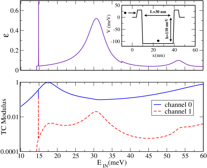
Figure 3: (Color online) Top panel: the entanglement $\varepsilon$ as a function of the initial energy of the incoming electron $E_{IN}$. The inset displays the potential $V(x)$ inside the scattering region: we consider a potential well 110 meV deep and 30 nm wide. Bottom panel: the modulus of the TC of the channels as a function of the initial kinetic energy of the incident electron: 0-th channel (solid line) and 1-st channel (dashed line). The scale of the abscissa is the same in the two panels.

By comparing the two panels in Fig. 3, it is clear that the resonances of the TCs play a key role in the entanglement formation. In particular, the behavior shown by the entanglement in correspondence of a Fano resonance is very different from the one exhibited at a Breit-Wigner resonance. When $E_{IN}$ is around 15 meV, a Fano resonance of the TC is observed for channel 0. To better understand this phenomenon, we report in the top panel of Fig. 4 a zoom of the curves of modulus and phase (the latter was not shown in Fig. 3, for clarity) of the TCs of the two channels. It is worth noting that, unlike the case of the single-channel scattering, here the modulus of the TC attains small but non zero values before the maximum, which, in turn, results to be significantly lower than 1. The TC of channel 1 shows, in correspondence of the Fano resonance of channel 0, a Breit-Wigner resonance characterized by a phase change of about $\pi$. In the energy interval around 15 meV the behavior of the quantum correlations, appearing in the systems as a consequence of the scattering, is peculiar (see the top panel of Fig. 4). In fact when the modulus of the TC of the channel 0 reaches its lowest value, the entanglement curve presents a minimum. Such a minimum is placed between two very close maxima, where the entanglement (evaluated, as usual, by means of the von Neumann entropy of the reduced density matrix) is equal to $\ln{2}$. This value indicates the condition of maximal entanglement in a two-channel scattering. Such a condition is reached when $|c_{0}|^{2}$ and $|c_{1}|^{2}$, i.e. the probabilities that the scattering occurs through the channel 0 or 1, respectively, are equal, and it implies that the lack of knowledge about the state in the one-particle subspace is maximum. We also report, in the top panel of the Fig. 4 (dashed line), the ratio of the two transmission probabilities: the entanglement is maximum when the scattering probabilities in the two channels are the same, as indicated by the horizontal dotted line drawn as a guide for the eyes. What we found here is in agreement with previous analyses on the two-electron entanglement production in two-electron systems for a two-channel scattering model, where both particles are injected in only one of two leadsOli ; Lopez . In fact, also in those cases, the entanglement shows a maximum when the transmission probabilities for the two channels are identical, while it vanishes in correspondence of the single-particle resonances, where there is no uncertainty about the energy of the particle.

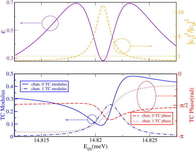
Figure 4: (Color online) Top panel: the entanglement $\varepsilon$ (solid line) and ratio between the probabilities of finding the scattered particle in the transmission channel 1, $|c_{1}|^{2}$, and 0, $|c_{0}|^{2}$ (dashed line), against the initial energy of the incoming electron $E_{IN}$, close to a resonant condition. Note that, while $\varepsilon$ can range from 0 (no entanglement) to $\ln{2}$ (maximally entangled state), the bottom of the left scale is set to 0.25 to optimize the magnification effect in the figure. The horizontal dotted line is a guide for the eyes indicating the point of equal scattering probabilities for the two channels, i.e. 1 in the left ordinates axis. Bottom panel: TC of the two channels as a function of $E_{IN}$ around a Fano resonance. The solid and the dash-dotted lines represent the modulus of TC of the channel 0 and 1 respectively, and refer to the left ordinate axis; the dashed and the dotted lines represent the phase of the TC of channel 0 and 1, respectively, and refer to the right axis.

Figure 3 shows that the TC of the channel 0 presents a Breit-Wigner resonance for $E_{IN}\simeq 17.5$ meV. Even if the modulus of the TC becomes equal to 1, the entanglement curve does not display maxima or minima. This is due to the fact that the Breit-Wigner resonance of the TC of channel 0 does not influence the TC of channel 1, which does not show, at the specific energy, resonances of any kind. Therefore, the scattering phenomena taking place in the energy interval around 17.5 meV do not play a special role into entanglement formation of the two-particle system. Such a behavior is in agreement with the one observed in other works, showing that the maximal value of the conductance does not always correspond to the maximal entanglement Ryc .

III.2 Multi-channel scattering

Let us consider now, the case of a multi-channel scattering (the scattered particle can leave the QD with more than two energies), and let us investigate the different roles played by the Fano and Breit-Wigner resonances in the entanglement formation.

Here, we consider a potential well 150 meV deep and 40 nm wide, as reported in the inset of Fig. 5. For $E_{IN}$ around 21 meV, the scattering passes from a two-channel to a three-channel process, and this transition is characterized by a sharp increase of the entanglement. The same behavior is found at $E_{IN}=40$ meV, where an additional transmission channel is switched on (see Fig. 5). This is in agreement with the results of the previous section and may be considered representative of a more general behavior, occurring whenever a new channel becomes effective in the scattering process.

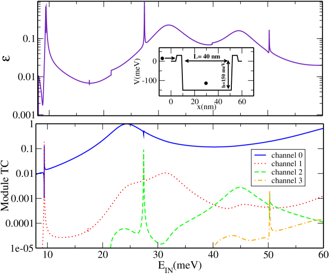
Figure 5: (Color online) Top panel: the entanglement $\varepsilon$ as a function of the initial kinetic energy of the incoming electron $E_{IN}$. The inset shows the profile of the potential $V(x)$ in the scattering region: the potential well is 150 meV deep and 40 nm wide. Bottom panel: modulus of the TC of the four channels as a function of $E_{IN}$: channel 0 (solid line), 1 (dotted line), 2 (dashed line) and 3 (dash-dotted line).

The quantum correlations appearing in the system, as a consequence of a multi-channel scattering, for the energy values around a Fano resonance show some differences with respect to the two-channel process. In Fig. 6 we report the curves of the entanglement and, in the insets, the modulus and phase of the TCs of the three channels (0, 1, 2 from top to bottom) against $E_{IN}$, in the energy region around $E_{IN}=27.5$ meV, where a Fano resonance occurs for channel 0. In fact, we observe, from the uppermost inset that also in this case the modulus of the TC has a local minimum before reaching the maximum. The type of resonances of channels 1 and 2 (middle and bottom insets) cannot be clearly identified by the module of their transmission coefficients, whose peaks are almost symmetric. However, it is clear for the transmission phases, that channel 1 exhibits a Fano resonance, with the phase essentially unchanged through the peak, while channel 2 shows a Breit-Wigner resonance, with a global phase variation of $\pi$. We stress that, unlike the two-channel scattering case, here the entanglement does not show a minimum. Such a behavior can be ascribed to the fact that, when the modulus of the TC of channel 0 is small, the TCs of the other two channels attain values comparable to each other. This means that the probabilities of finding the scattered particles in those channels are almost equal, and there is still a lack of knowledge about the state of the one-particle subsystem. Furthermore, we note that here the entanglement presents a single maximum whose value exceeds $\ln{2}$. Actually, the fact that the number of degrees of freedom is larger than 2 increases the uncertainty about the constituents of the system; in fact Eq. (6) gives a maximum value for the amount of quantum correlations that is larger for a larger number of possible states. For example, a system of two qutrits is able to attain a larger value of $\varepsilon$ than a two-qubit system. The ability to tailor not only the degree of the entanglement, but also the number of possible states of the two subsystems, by independently tuning $E_{IN}$ and the QD confining potential, could also have implications beyond the theoretical estimation of the entanglement. The behavior described above is repeated at $E_{IN}\simeq 50$ meV where two Fano resonances occur for the second and third channel in a four-channel scattering (Fig. 5).

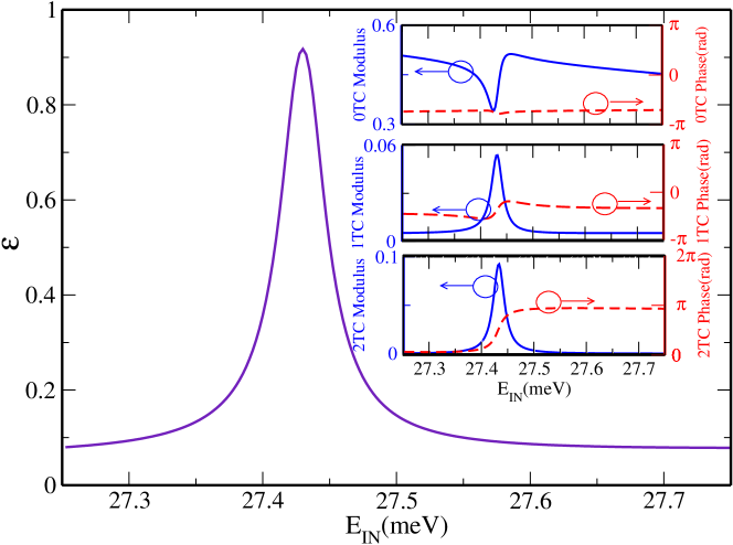
Figure 6: (Color online) The entanglement $\varepsilon$ as a function of $E_{IN}$ around a Fano resonance of the TC of channel 0in a three-channel scattering. The insets display the modulus (solid line, left axis) and phase (dashed line, right axis) of TC of three channels (0, 1, 2 from top to bottom) in the same energy range of the main graph.

It is worth noting that, in correspondence of a Breit-Wigner resonance in the channel 0 for $E_{IN}=25$ meV, no additional resonance occur in the other channels and the entanglement does not present maxima or minima as it can be clearly seen from the upper panel of Fig. 5. Therefore also in the case of multi-channel processes, the Breit Wigner resonance seems not to induce sharp variations of $\varepsilon$.

IV Conclusions

The controlled production and detection of entangled particles in the solid state environment represents an experimental challenge. In this spirit, various proposals for producing bipartite entangled fermionic systems have been advanced, on the basis of different physical mechanisms requiring a direct interaction between particles bus ; Oli ; raa ; bor2 ; Rasm ; Lopez . In this paper we have investigated the quantum correlations appearing, as a consequence of a Coulomb scattering, between two electrons having the same spin, in a system of physical interest, where the degree of the entanglement results to be controllable by a proper tuning of the carrier energy and of the QD potential. Such a system consists of a quasi 1D double-barrier resonant tunnelling device, where an electron incoming from one lead is scattered by the potential structure and, via the Coulomb interaction, by another electron bound in the QD.

The numerical procedure, used to solve the model, is a generalization of the quantum transmitting boundary method Berton ; Lent . It permits us to obtain the reflection and transmission amplitudes of each scattering channel, for various configurations of the potential, as a function of the initial energy of the incoming electron. However, we stress that, unlike the approaches followed by Lopez et al. Lopez and by Oliver et al. Oli , here we did not use the reflected component of the scattered electron wavefunction to evaluate the entanglement of the two-particle system, but we estimated the quantum correlations showing up between the QD eigenstates and the transmitted parts of the electron wavefunction. Furthermore, this procedure makes it possible to investigate the role played by the resonances of the transmission spectra into the entanglement. Although our numerical analysis has been performed by using the GaAs material parameters, they can be considered representative of a more general behavior.

Our simulations show that the entanglement depends upon the kind of the resonance appearing in the transmission spectrum. A single Breit-Wigner resonance is found not to induce peculiar effects on quantum correlations. On the contrary, in correspondence of a Fano resonance of one of the TCs, not only the other channels TCs exhibit local maxima, but also the entanglement presents sharp peaks. Such a behavior can be related to the nature of the resonances themselves. In fact a Breit-Wigner resonance is essentially a one-particle effect, showing up also in a single-electron scattering. On the other hand, a Fano resonance is a genuine multi-particle phenomenon, due to electron-electron correlation, and is not present for single-particle systems.

Furthermore, we showed that the appearance of quantum correlations in our system is also affected by the number of the transmission channels, i.e. the number of possible energy levels of the scattered particle (and, due to the energy conservation, of the bound particle). In fact, the entanglement shows a sharp increase whenever a new channel is turned on. Moreover, its behavior for energy values around a Fano resonance is found to depend upon the kind of process: two- or multi-channel scattering. For the two-channel case, the entanglement presents a minimum between two close maxima, which indicate the maximal uncertainty about the state of the system. In the multi-channel case, a single maximum of the entanglement, with no minima, is observed. When the energy levels of the scattered and bound electrons are only two, the minimum of the entanglement is found in correspondence of the local minimum of the TC of the Fano resonant channel. In this case it maximizes the possibility to ascribe specific energy states to the subsystems. On the other hand, for a multi-channel scattering, a minimum of TC of a Fano resonant channel does not imply a decrease of uncertainty about the subsystems, since the TCs of the other non Fano resonant channels attain values comparable to each other.

Finally, the results of our paper suggest that the manipulation of Fano resonances and of the number of scattering channels may allow to significatively influence the degree of entanglement between the transmitted electrons and the QD. A promising development of the present work could be the study of the entanglement in the case of scattering of a single electron by a few charges confined in the QD, in connection with experimental results obtained for the coherent components of the transmitted current in the case of the multi-occupancy of the dot Kon ; Aik . In the latter case, with three or more particles in the system, the spin degrees of freedom cannot be factorized and their inclusion in our approach, although quite feasible, results very challenging form the computational point of view.

References

- (1) A. Einstein, B. Podolsky and N. Rosen, Phys. Rev. 47, 777 (1935).
- (2) D. Bouwnmeester, A. Ekert and A. Zeilinger, The Physics of Quantum Information (Springer-Verlag Berlin and Heidelberg GmbH & Co. K Springer, Germany, 2000)
- (3) W.H. Chan and C.K. Law, Phys. Rev. A 74, 024301 (2006).
- (4) R. Lo Franco, G. Compagno, A. Messina, and A. Napoli, Phys. Rev. A 72, 053806 (2006).
- (5) F. Buscemi, P. Bordone and A. Bertoni, Phys. Rev. A, 73, 052312 (2006).
- (6) A. Bertoni, P. Bordone, R. Brunetti, C. Jacoboni, and S. Reggiani, Phys. Rev. Lett., 84, 5912 (2000)
- (7) P. Bordone, A. Bertoni and C. Jacoboni, J. Comp. Elec., 3, 407 (2004)
- (8) W.D. Oliver, F. Yamaguchi, Y. Yamamoto, Phys. Rev. Lett. 88,037901 (R) (2002).
- (9) A. Ramsak, J. Mravlje, R. Zitko, and J. Bonca, Phys. Rev. B 74,241305(R) (2006).
- (10) A. Ramsak, I. Sega and J.H. Jefferson, Phys. Rev. A, 74, 010304(R) (2006).
- (11) D. Loss and D.P. Di Vincenzo, Phys. Rev. A, 57, 120 (1998).
- (12) A. Imamoglu et al., Phys. Rev. Lett., 83, 4204 (1999).
- (13) G. Bester, and A. Zunger, Phys. Rev. B 72, 165334 (2005).
- (14) B.J. van Wees et al., Phys. Rev. Lett., 60, 848 (1998).
- (15) U. Meirav, M.A. Kastner, and S.J. Wind, Phys. Rev. Lett., 65, 771 (1990).
- (16) W.G. van der Wiel et al., Rev. Mod. Phys., 75, 1 (2003).
- (17) B. Lassen and A. Wacker, e-print cond-mat/0703286v1
- (18) H. Aikawa, K. Kobayashi, A. Sano, S. Katsumoto, Y. Iye, Phys. Rev. Lett., 92, 176802 (2004).
- (19) A. Yacoby, M. Heiblum, D. Mahalu and H. Shtrikman, Phys. Rev. Lett, 74, 4047 (1995).
- (20) M. Avinun-Kalish, M. Heiblum, O. Zarchin, D. Mahalu and V. Umansky, Nature, 436, 529 (2005).
- (21) I. Neder, M. Heiblum, D. Mahalu and V. Umansky, Phys. Rev. Lett., 98, 036803 (2007).
- (22) J. Gores et al., Phys. Rev. B, 62, 2188 (2007).
- (23) C. Fuhner, U.F. Keyser, R.J. Haug, D. Reuter and R.J. Haug, e-print cond-mat/0307590
- (24) M.L. Ladron de Guevara and P.A. Orellana, Phys. Rev. B, 73, 205303, (2006).
- (25) A. Bertoni and G. Goldoni, J. Comput. Electron., 73, 205303 (2006).
- (26) J.U. Nockel and A.D.Stone, Phys. Rev. B, 50, 17415 (1994).
- (27) U. Fano, Phys. Rev., 124, 1866 (1961).
- (28) G. Breit and E. Wigner, Phys. Rev., 49, 519 (1936).
- (29) P.I Tamboronea and H. Metiu, Europhys. Lett., 53, 776 (2001).
- (30) A. Rycerz, Eur.Phys. J.B, 52, 291 (2006).
- (31) L.D. Contreras-Pulido and F. Rojas, J. Phys.: Condens. Matter 18, 9971 (2006).
- (32) T. Ihn, C. Ellenberger, K. Ensslin, C. Yannouleas, U. Landman, D.C. Driscoll, and A.C. Gossard, Int. J. Mod. Phys., 21, 1316 (2007).
- (33) A. Lopez, O. Rendon, V.M. Villaba and E. Medina, Phys. Rev. B, 75, 033401 (2007).
- (34) M.T. Bjork, C. Thelander, A.E. Hansen, L..E Jensen, M.W. Larsson, L.R. Wallenberg and L.G. Samuelson, Nano Lett., 4, 1621 (2004).
- (35) M.M. Fogler, Phys. Rev. Lett., 94, 56405 (2005)
- (36) C.S. Lent and D.J Kirkner, J. Appl. Phys, 67, 6353 (1990).
- (37) A. Bertoni and G. Goldoni, Phys. Rev. B, in press (2007).
- (38) A. Peres, Quantum Theory: Concepts and Methods (Kluwer Academy Publishers, The Netherlands, 1995.)
- (39) J. Schliemann, J.I. Cirac, M. Kus, M. Lewenstein and D. Loss, Phys. Rev. A 64, 022303 (2001).
- (40) F. Buscemi, P. Bordone and A. Bertoni, Phys. Rev. A, 75, 032301 (2007).
- (41) K. Eckert, J. Schliemann, D. Bruss, and M. Lewenstein Annals of Physics 299, 88-127 (2002)
- (42) J. Konig and Y. Gefen, Phys. Rev. Lett., 86, 3855 (2001)